Article

A New Remote Sensing Index for Assessing Spatial Heterogeneity in Urban Ecoenvironmental-Quality-Associated Road Networks

1
College of Transportation and Civil Engineering, Fujian Agriculture and Forestry University, Fuzhou 350108, China
2
College of Forestry, Fujian Agriculture and Forestry University, Fuzhou 350002, China
*
Author to whom correspondence should be addressed.
Land 2022, 11(1), 46; https://doi.org/10.3390/land11010046
Submission received: 1 December 2021 / Revised: 23 December 2021 / Accepted: 27 December 2021 / Published: 29 December 2021
(This article belongs to the Topic Climate Change and Environmental Sustainability)

Abstract

:
Although many prior efforts found that road networks significantly affect landscape fragmentation, the spatially heterogeneous effects of road networks on urban ecoenvironments remain poorly understood. A new remote-sensing-based ecological index (RSEI) is proposed to calculate the ecoenvironmental quality, and a local model (geographically weighted regression, GWR) was applied to explore the spatial variations in the relationship between kernel density of roads (KDR) and ecoenvironmental quality and understand the coupling mechanism of road networks and ecoenvironments. The average effect of KDR on the variables of normalized difference vegetation index (NDVI), land surface moisture (LSM), and RSEI was negative, while it was positively associated with the soil index (SI), normalized differential build-up and bare soil index (NDBSI), index-based built-up index (IBI), and land surface temperature (LST). This study shows that rivers and the landscape pattern along rivers exacerbate the impact of road networks on urban ecoenvironments. Moreover, spatial variation in the relationship between road network and ecoenvironment is mainly controlled by the relationship of the road network with vegetation and bare soil. This research can help in better understanding the diversified relationships between road networks and ecoenvironments and offers guidance for urban planners to avoid or mitigate the negative impacts of roads on urban ecoenvironments.

1. Introduction

Roads appear as conspicuous objects across the world. Official statistics are staggering, with 4.8 million km2 of highways in 2018 in China, 73,100 km2 more than that in 2017, and a highway density of 50.48 km/100 km2 in 2018, increasing 0.76 km/100 km2 from 2017. China’s mountainous areas, including hills and plateaus, cover an area of 6.636 million km2, accounting for 69.1% of the total land area in the country, which means that these road networks might affect the ecoenvironment of a considerable part of the country’s earth surface. Previous studies suggest that roads might affect the ecoenvironment of nearly 15–20% of the total land area of the United States [1] and nearly 16% of the Netherlands [2]. Similarly, roads might impact approximately 20% of China’s land ecosystems [3]. It is projected that a further 25 million km2 of roads will be constructed around the world by 2050 [4]. Such rapid extension of roads may impose serious ecoenvironmental threats and challenges in the future [5], including accelerating the fragmentation and degradation of vegetation, further affecting the urban thermal and humidity environment. Roads are clearly something worth understanding. To effectively avoid or mitigate the negative impacts of roads, it is essential to develop a systematic research framework to fully understand the impacts of roads on ecoenvironments and their causal mechanisms [6]. Many previous studies focused on exploring landscape dynamics associated with road networks [6,7,8,9]. However, ecoenvironmental effects on land use and land cover and thermal and humidity environments, especially an integrated measure of ecoenvironments emanating from roads, are not fully investigated [1,7,8]. There is a huge knowledge gap in the ecoenvironmental effects of road networks in the heavy road sprawl zones in urban areas [9].
Roads have a wide array of ecological effects spreading through terrestrial and aquatic ecosystems [1]. First, road construction has a huge ecological impact early during land use and cover changes [10], causing local habitat loss and increasing disturbances in the surrounding landscape [11]. Moreover, road extension may induce landscape fragmentation by cutting landscapes into pieces [7]. Specifically, significant changes in landscape structure can be observed in most cases, such as decreasing the size of patches (core area size), increasing the number of patches (patch density), and simplifying or complexing the shape of patches (patch dimension) [5,12,13]. Reed et al. [14] quantified fragmentation caused by roads in Southeastern Wyoming with several landscape structure measures, such as the number of patches, mean patch area, and perimeter-related indices, indicating that forest fragmentation was aggravated by cutting large plaques into smaller pieces and by transforming interior forest habitats into forest edges. Reed et al. [14] also indicated that fragmentation could be reduced by minimizing or rerouting road construction. Karlson Mörtberg [15] explored the potential effects of fragmentation and disturbance of roads on the landscape in Sweden, revealing the main consequence of habitat loss of road effects. The destructive effects of roads on wildlife were reported as a major crisis of global biodiversity [16].
From many perspectives, the detrimental impact of roads on nature (both terrestrial and aquatic) ecosystems was fully explored [6,15]. However, the ecoenvironmental impact of road networks on urban areas has received little attention [9]. Previous studies on the landscape effect of roads emphasized spatial structures and pattern dynamics, while little analysis has been conducted on the urban area’s ecoenvironmental function or quality, even with a dense road network. Wu et al. [17] assessed the effects of a highway on landscape patterns in a town of Taiwan province. They discovered that the combination of highway construction and its subsequent urbanization had caused landscape isolation and fragmentation in the study area. Besides the biological ecosystem, roads significantly impact the abiotic ecosystem, such as air, water, and temperature [1]. For example, the direction of the road affects the ventilation of a city, which affects the thermal field distribution of a city. Moreover, road motor vehicles are a main source of carbon emissions [6]. Nearly 20% of the world’s carbon dioxide (CO2) emissions are generated from road traffic; the proportion was nearly 8% in China in 2015, and these emissions are increasing annually [8]. This may aggravate the deterioration of the urban ecoenvironment, such as with the heat island effect [18]. Severe health consequences for humans, coupled with limited knowledge of how these landscape fragmentations caused by roads and road traffic pollutions jointly affect ecoenvironmental quality in urban areas, highlight an urgent need to fill the knowledge gap of the relationship between roads and ecoenvironmental quality from a landscape perspective. This sheds light on the mitigation measures for urban ecoenvironmental planning.
The need for sustainable planning and decision making for urban areas stresses the need for the construction of a framework to effectively address ecoenvironmental quality. Environmental impact assessment (EIA) and strategic environmental assessment (SEA) are two legal frameworks to evaluate, project, and mitigate the adverse ecological effect of transport infrastructure; the Convention on Biological Diversity (CBD), the European Landscape Convention (ELC), and the EU Biodiversity Strategy (BS) also address the treatment of ecological impacts [15]. These analytical frameworks were extensively employed in environmental assessment studies [19,20]. However, these frameworks emphasized habitat protection and the increasing landscape connectivity for conserving biodiversity and ecosystem services. Moreover, these methods are only applicable to specific projects or administrative divisions, and they cannot explain the spatial distribution of ecological conditions and their changes for a region [21,22]. These problems are extremely important for proposing an effective index to identify spatial variation in the ecoenvironmental impact of roads.
At present, the utility of remote-sensing indicators as a tool to identify the impacts of roads in ecoenvironmental quality remains a challenge, since their relationships may vary across the study area (i.e., spatial nonstationarity). To our knowledge, spatial nonstationarity in the relationships between roads and ecoenvironmental quality is rarely explored. Therefore, taking the city of Fuzhou as a case, we employed geographically weighted regression (GWR), a local model, to explore the spatial nonstationarity in the relationships between the kernel density of roads (KDR) and several ecological indicators across the study area, including RSEI, normalized difference vegetation index (NDVI), and land surface temperature (LST). The following questions were explored: (1) Do the relationships of roads between RSEI and its constituent factors vary with locations across the study area? (2) Do trade-off (i.e., negative) or synergistic (i.e., positive) relationships between the two regressors predominate? (3) How are their relationships distributed?
Solving and understanding the three above questions could improve our knowledge of urban ecoenvironmental patterns and enhance our capabilities in road-network and urban planning.

2. Materials and Methods
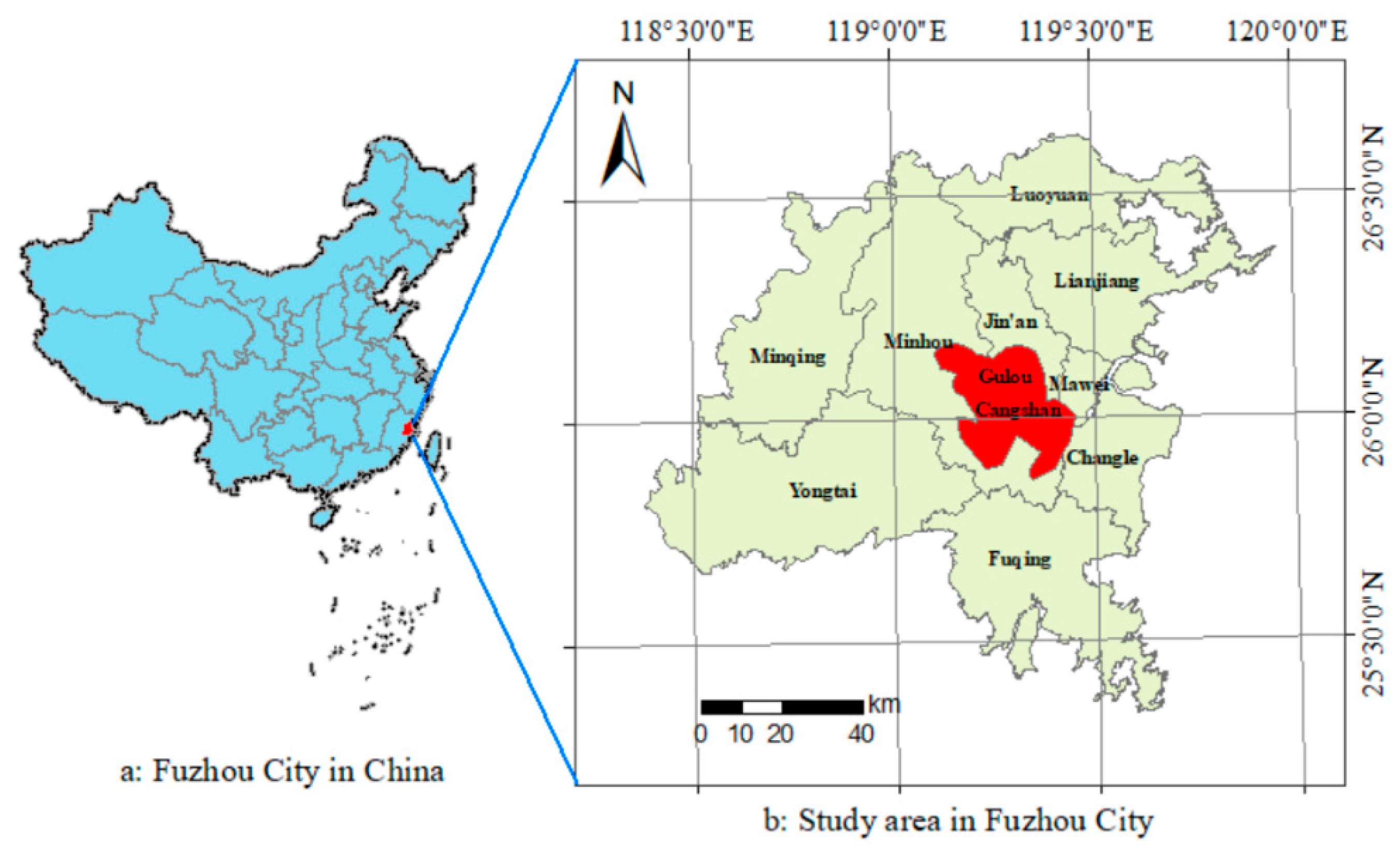
2.1. Study Area

Fuzhou is the capital and the largest prefecture-level city in the Fujian province of China (Figure 1), which is in the west coast of the Taiwan Strait and in the lower reaches of the Minjiang River. Fuzhou has experienced rapid urbanization over the past three decades, with built-up area increasing more than 15 times from 22 km2 in 1978 to 357 km2 in 2018 [23]. Urban sprawl combined with the basinlike topography to transform it into a new “stove” in China. Therefore, these features of the city make it a particularly interesting case for exploring the spatial relationships between roads and the ecoenvironmental quality. Average annual temperature is approximately 293.9 K. Annual precipitation varies widely from 796.5 to 1913.6 mm, with approximately one-third received in May and June. The study area (Figure 1b) is the downtown area of the city, with dense buildings and population. Ecoenvironmental quality has been dramatically deteriorating in the past two decades [24]. The city is one of the four new furnaces in China. Consequently, the study on spatial variations in the associations between ecoenvironment quality and road networks is necessary and may shed light on rapidly urbanizing global regions.

2.2. Data Resources and Pre-Processing

The Landsat OLI/TIRS image (Path = 119, Row = 42) used in this study was acquired on 25 June 2016 (2:32 pm local time) from the United States Geological Survey (USGS) [25]. Spatial resolution was 30 m per pixel. The cloudy cover of the image was 4.27%. Images were in Level 1B and systematically processed to provide geometric corrections prior to analysis. Images were composed of 11 bands, namely, the bands of visible light (4), the near-infrared (1), the short-wave infrared (2), the Pan (1), the cirrus (1) and the thermal infrared (2) bands. Clouds and their shadows were masked on the basis of very low temperature [23]. Water patches were marked on the basis of the modified normalized difference water index (MNDWI) [26]. For more detailed steps, please refer to our published literature [23,27,28]. The road-network dataset was obtained from OpenStreetMap, and road-network data for the period correspond to Landsat data. Road-network data were topologically checked before density analysis, and the integration tool was employed to merge the double line into a single line of roads to avoid double counting on the same roads.

2.3. Indicator Selection

Recent advances in the availability of satellite-based datasets and remote-sensing technology have provided a powerful tool to identify ecoenvironmental status on the pixel level with complete coverage for various ranges, from local to global [27,29]. Therefore, remote-sensing techniques were extensively employed in ecoenvironmental observations on Earth [28,30]. A number of remote-sensing indices, including single-factor (e.g., enhanced vegetation index, EVI; leaf area index, LAI; normalized difference vegetation index, NDVI; land surface temperature, LST) [31,32,33,34] and aggregated (e.g., MODIS global disturbance index, MGDI; forest disturbance index, DI; scaled drought condition index, SDCI) indices [35,36,37]. More recently, Xu et al. [21] coined a remote-sensing-based ecological index (RSEI) by integrating the four indicators of greenness, wetness, dryness, and heat. The applications of RSEI suggest that it can effectively assess ecoenvironmental conditions in different regions [21,22,27,28].
Therefore, we selected RSEI as our key indicator to understanding the coupling mechanism of road networks and ecoenvironments. Some other ecological indicators that are widely applied to urban ecological evaluation were selected to compare with the results of RSEI, including normalized difference vegetation index (NDVI), land surface temperature (LST), normalized differential build-up and bare soil index (NDBI), land surface moisture (LSM), soil index (SI), and index-based built-up index (IBI). The summary of all selected indicators and abbreviations is in Table 1.

2.4. Calculation of Remote-Sensing-Based Ecological Index

Remote-sensing-based ecological index (RSEI) is a synthetic index that quickly and quantitatively assesses a region’s ecoenvironmental quality and is based on the pressure-state-response framework (PSR) using principal-component analysis (PCA) [21,28]. RSEI is capable of overcoming the weaknesses of most of the previous ecological indicators, which merely measure the response of the ecosystem to anthropogenic stresses causing impairment. The RSEI is built upon the selection and measurement of indicators for three categories [28] (i.e., indicators of anthropogenic pressures, environmental states, and climatic responses), including greenness, dryness, heat, and humidity, which are represented by the normalized difference vegetation index (NDVI), normalized differential build-up and bare soil index (NDBSI), land surface temperature (LST), and land surface moisture (LSM), respectively. NDBSI was calculated by combining the soil index (SI) and index-based built-up index (IBI). All these indicators can be quickly obtained from Landsat datasets at the pixel level. The calculation formulas of these indicators and the synthesis of RSEI are detailed in the references [21,28].

2.5. Estimation of Road Kernel Density
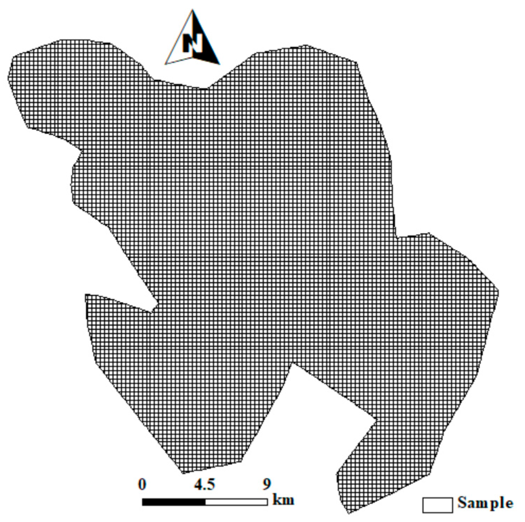
The kernel function is used to calculate the road-network density (i.e., KDR) per unit area on the basis of points to fit each point to a smooth cone-shaped surface by moving windows [40]. The used kernel function was adapted from the fourth-order kernel function used to calculate the point density described in Silverman’s book [41]. The search radius (bandwidth) of moving windows within which unit is calculated according to the Silverman rule of thumb spatial variable, which can effectively avoid spatial outliers (that is, points that are too far away from other points). The KDR map was produced in ArcGIS; the specific parameter design can be referred to in a previously published paper [42].

2.6. Sampling

Using ArcGIS software, a fishing net of 300 × 300 m was established as the sampling unit, with a total of 7796 samples for the study area (Figure 2). The Zonal Statistics as Table tool was employed to summarize the average values of all rasters within each sample of the datasets of each variable, and the statistical tables for all the variables were output. Then, all average values in the output tables were joined to the sample layer on the basis of the predetermined field. Thus, the sample layer had the attributes (i.e., the average value) of all variables at 300 × 300 m polygons, which can be used as an input feature in modeling spatial relationships in ArcGIS.

2.7. Regression Models

Both a global model (ordinary least squares, OLS) and a local model (GWR) were employed to examine the association between RSEI-associated indices (including NDVI, IBI, SI, NDBSI, LST, LSM, and RSEI) and KDR. OLS models were used to detect the overall relationship between the two regressors, while the GWR models were applied to identify the spatial heterogeneity in the interactions between the two regressors across locations [23]. Regression models were simulated in ArcGIS. The KDR was set as the independent variable, and NDVI, IBI, SI, NDBSI, LST, LSM, and RSEI were set as dependent variables in each separate model. In terms of GWR models, the adaptive kernel type was set, and the bandwidth of the kernel was determined using the Akaike information criterion (AICc). The goodness of the models was evaluated using the test indicators [23] of adjusted R-squared, AICc, residual squares, p-value, and Moran’s I.

3. Results

3.1. GWR and OLS Model Testing

Table 2 indicates the test results of the OLS and GWR models for fitting the associations between the KDR and the RSEI variables. The higher the adjusted R2, the smaller the AICc values of the GWR models against the OLS models, indicating a better goodness of the GWR models than that of the OLS ones. The relatively small values of Moran’s I (0.199–0.309) reveal the small spatial autocorrelation in residual squares (Figure 4B,D,F,H,J,L,N), indicating the random distribution in the residuals across the study area. Moreover, all seven GWR models were statistically significant at the 0.001 level, also indicating a high goodness fit for all GWR models. This supports the use of the GWR model in this study.

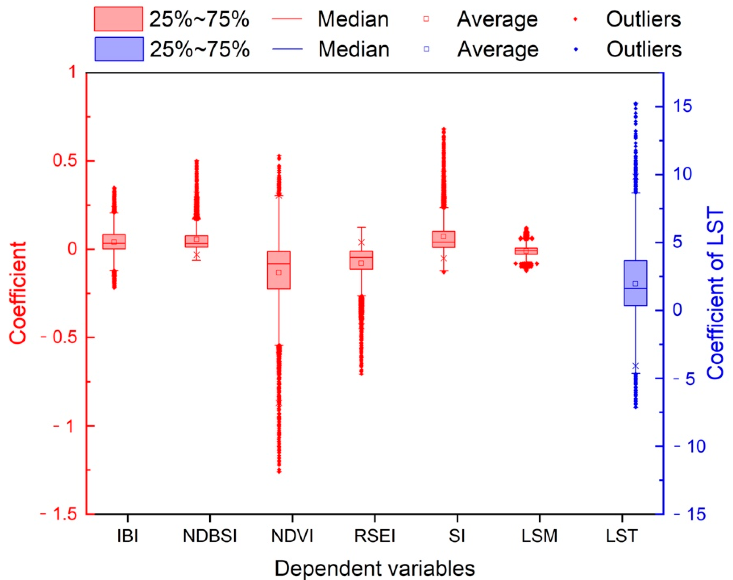
3.2. Summary of Coefficients of GWR Models

Figure 3 presents parameter descriptive statistics of the GWR models. These statistics can be used to compare the coefficient changes in different variables and reveal the variation in the coefficients in the study area. Specifically, the impacts of KDR on all the RSEI indicators were both positive and negative across the study region. Excluding the variable of LST, whose values were not between −1 and 1, the impacts of KDR on the other variables (from large to small) were in the order of NDVI, RSEI, SI, NDBSI, IBI, and LSM. The average effect of KDR on the variables of NDVI, LSM, and RSEI was negative, while it was positive on the variables of IBI, SI, NDBSI, and LST.

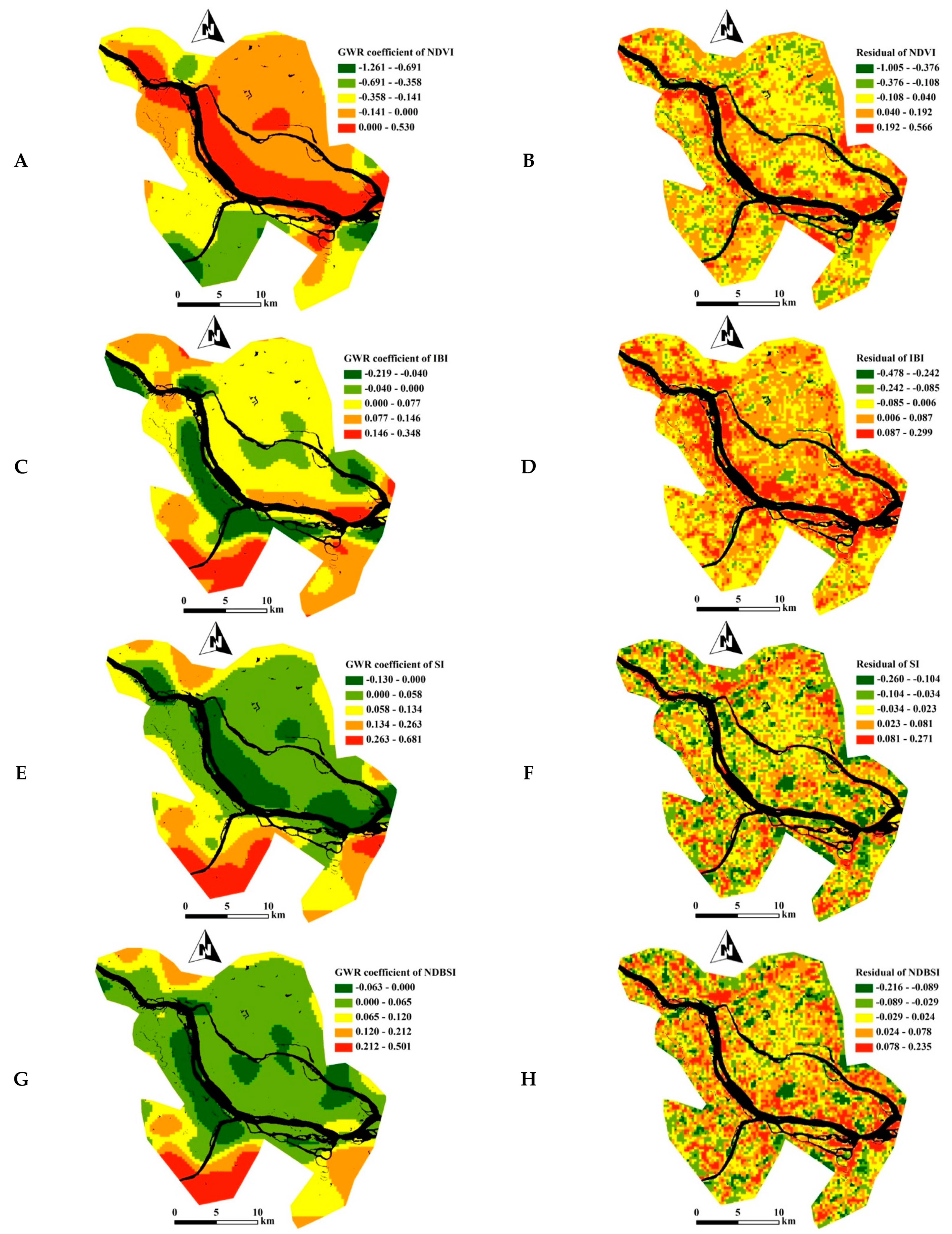
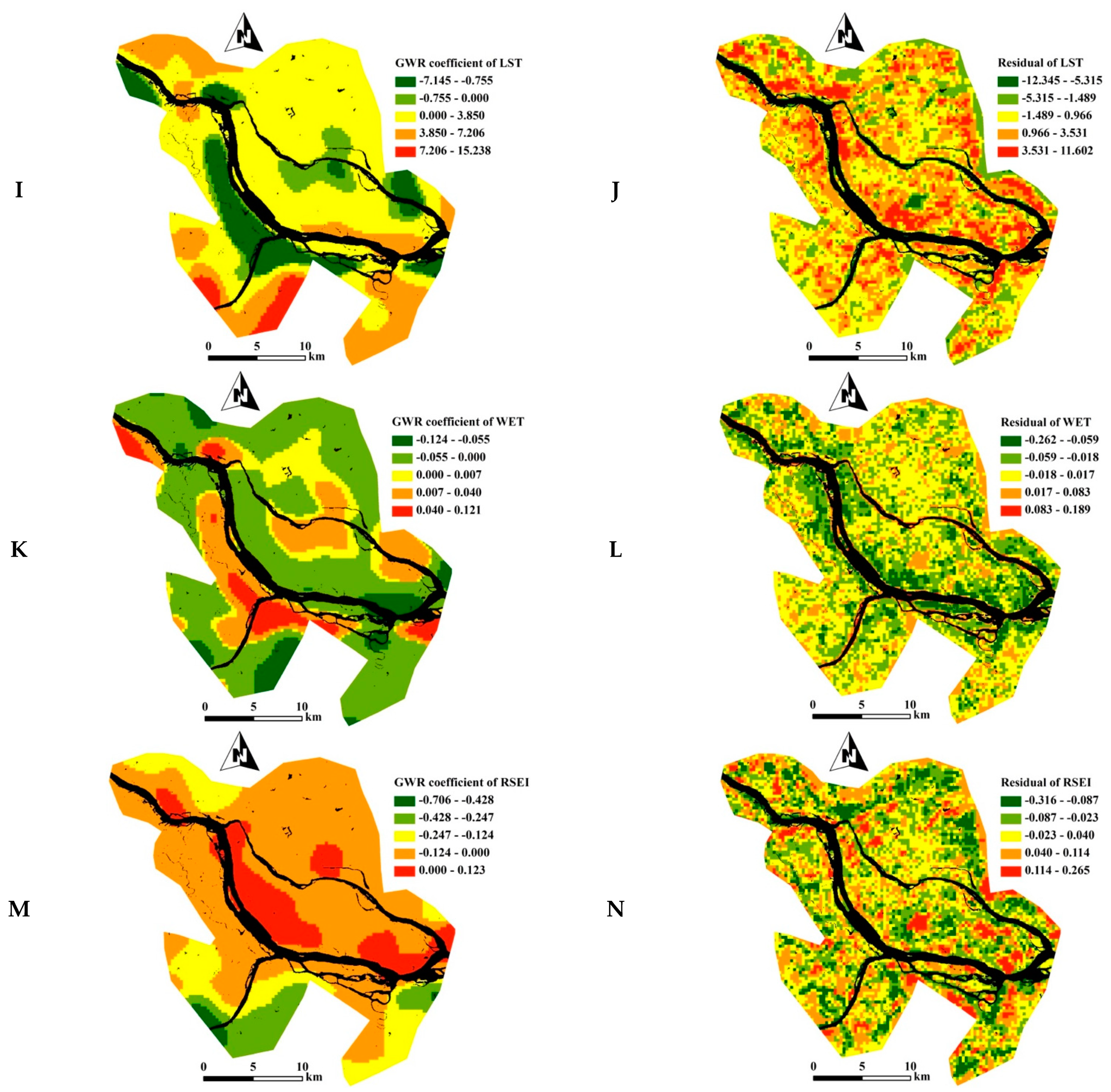
3.3. Spatial Variations in the Response of RSEI Indicators to KDR

GWR regression coefficients were mapped at grid level as shown in Figure 4A,C,E,G,I,K,M. In these maps, the Jenks method was employed to classify the coefficients into five categories, with zero being artificially set as a demarcation point to distinguish the positive and negative effects.
Figure 4A,B show that the negative relationships between KDR and NDVI were distributed across most of the study area. This indicated that the NDVI increased gradually as KDR decreased, whereas the decreasing rates significantly varied across the study region. The negative correlation coefficients were noticeably higher in the southern part (i.e., green clusters), while the negative correlation coefficients were obviously lower in the extensively northern areas (i.e., brown clusters), where the central urban area is. However, a narrow stripe (2 km or so) located close to the river exhibited positive correlation between KDR and NDVI, indicating that the NDVI gradually increased as the KDR increased.
Figure 4C,D indicate that the positive relationships between KDR and IBI were dominantly distributed in the study area, which indicates that the IBI gradually increased as the KDR increased. The figure also shows that the impact of the KDR on the IBI varied significantly across the region, with positive correlation coefficients being noticeably higher in the boundary regions (i.e., red clusters) while being obviously lower in the extensive central and northern areas (i.e., yellow clusters). However, a narrow stripe (2 km or so) located close to the river was negatively correlated with the IBI, indicating that the IBI decreased gradually as the KDR increased.
Figure 4E,F reveal spatial variations in the relationships between KDR and SI. The figure reveals that the positive correlations between KDR and SI occupied most of the study area. The positive correlation presented a basinlike trend, with low values in the middle and high values in the surroundings of the study area. Similar to Figure 4A,B, there was also a narrow stripe closer to the river, indicating noticeably negative associations between KDR and SI and that the SI gradually decreased as the KDR increased.
Figure 4G,H indicate spatial variations in the relationships between KDR and NDBSI. The law of the spatial distribution was similar to that of Figure 4C,D. The figure shows that the positive correlation prevailed over the negative correlation in the study area. The positive correlation coefficients were noticeably higher in the boundary regions (i.e., red, brown, and yellow clusters), while they were obviously lower in the extensive central and northern areas (i.e., green clusters). Moreover, there was a narrow stripe (2 km or so) located close to the river that was negatively correlated with the NDBSI.
Figure 4I,J indicate a similar pattern in the relationships between KDR and LST with those between KDR and IBI (Figure 4C,D). In Figure 4I,J, warm colors (i.e., red, brown, and yellow) represent a positive relationship, and the cool color (i.e., green) indicates a negative relationship. Similar to Figure 4C,D, positive correlation prevailed over the negative correlation in the study area. The positive correlation coefficients were noticeably higher in the boundary regions (i.e., red, brown, and yellow clusters), while being obviously lower in the extensive central and northern areas (i.e., green clusters). Moreover, there was a narrow stripe (2 km or so) located close to the river that was negatively correlated with the LST.
Figure 4K,L reveal the spatial variations in the relationships between KDR and LSM. The relationships demonstrated that the negative relationship between KDR and LSM was distributed in most of the study areas, indicating that the LSM decreased with the increase in KDR. However, there was also a part of the study areas showing a positive relationship, distributed in the central area of the urban area and the southern part of the study area, where it was distributed in negatively correlated places of the KDR and the IBI and the KDR and the LST (Figure 4C,D,I,J).
Figure 4M,N indicate the pattern of the relationships between KDR and RSEI, similar with those of KDR and NDVI (Figure 4A,B), while they were the opposite of those of the KDR and the SI (Figure 4E,F). In Figure 4M,N, the red cluster represents a positive relationship, which was a narrow stripe (2 km or so) located close to the river, while the other areas were all in negative associations. Similar to Figure 4A,B,E,F, the negative or positive correlation coefficients were noticeably higher in the southern part (i.e., green or red clusters), while the negative or positive correlation coefficients were obviously lower in the extensive northern areas (i.e., brown and yellow or light green clusters).

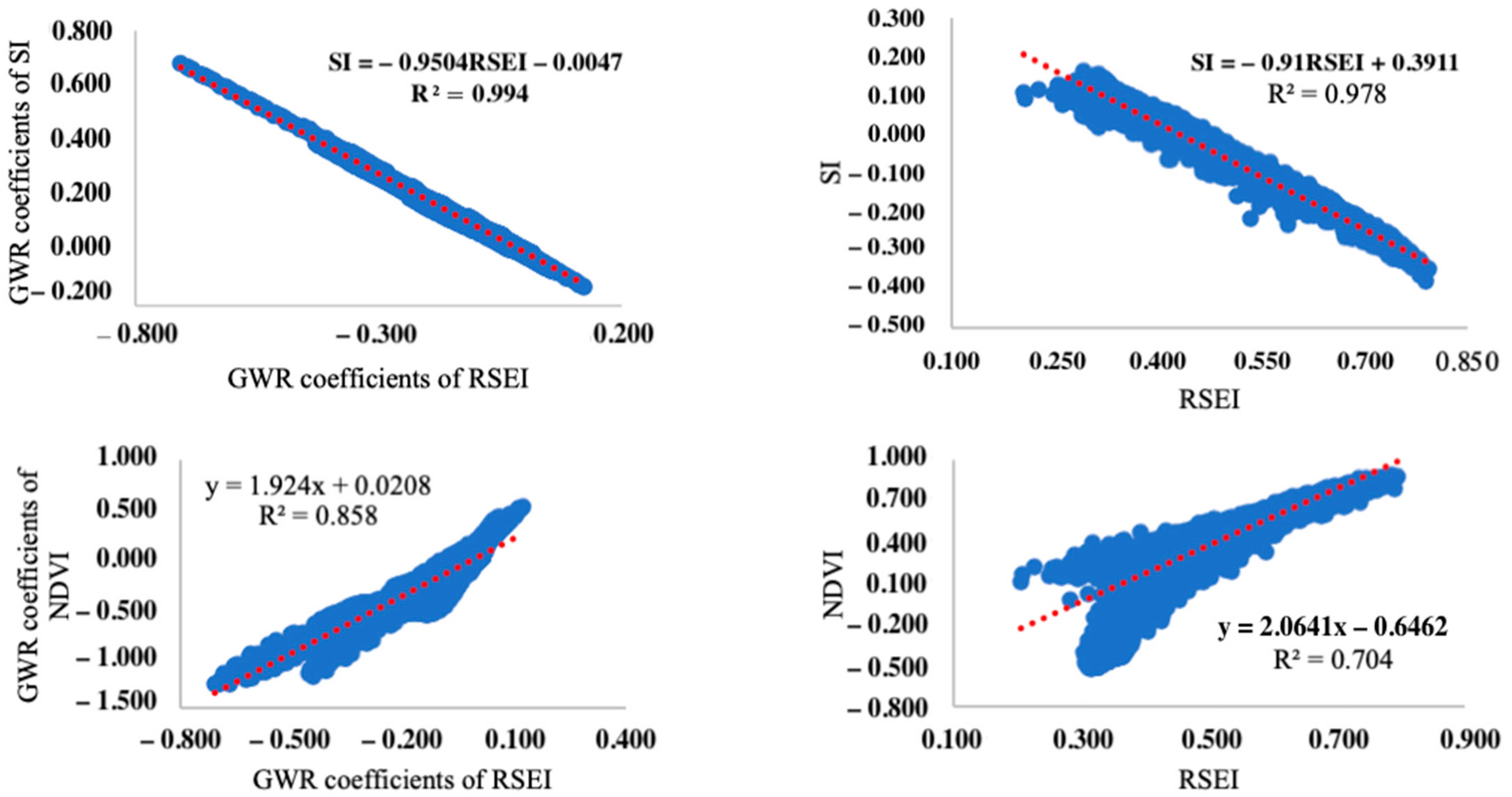
3.4. Correlation Analysis between Ecological Indicators

To investigate the interactions between ecoenvironmental indicators, Pearson’s correlation analysis and a 2D scatter plot were employed here. Sampling was randomly implemented using a 10 × 10 grid across the study area. Results of Pearson’s correlation analysis (Table 3) showed that SI and RSEI values and their GWR regression coefficients had the greatest correlation among all other pairs of variables, with R2 being as high as −0.989; the NDVI and RSEI also had strong positive relationships. The scatter plots also show high linear relationships between them (Figure 5). Due to water and soil loss upstream of Minjiang River, there is much sediment in the river body, leading to the distribution of the SI to be different from that of other indices, with the differences of the SI values between the land surface and water body being much smaller than those of the other indices. For example, ecoenvironmental indicators such as NDVI, IBI, and NDBSI showed a binary distribution pattern between land surface and water body.

4. Discussion

Regression results showed that the OLS models indicated statistically significant relationships between KDR- and RSEI-composed indicators (R2 = 0.013–0.168, p-value = 0.05), while the GWR model showed considerably stronger relationships from the same datasets (R2 = 0.314–0.564, p-value = 0.001), highlighting a tendency of spatial nonstationarity in the relationships (Table 1). The main reason is conventional ordinary least-squares regression models assuming spatial stationarity in the relationship between regressors. Such an assumption may often become untenable by ignoring the local variations in variables in each sample site, particularly in large-scale studies based on remote-sensing images [43,44,45]. Local statistical approaches (e.g., GWR) can be more appropriate than global techniques (e.g., OLS) if the relationship is spatially non-stationary [46]. GWR can capture spatial variations in the relationship between variables by including the spatial coordinates of the sample grids in the model. Therefore, GWR has huge potential in studies using remote-sensing data, as such data commonly have explicit spatial characteristics. However, the method is not a panacea with essential issues, such as the calculation of weight matrix, in processing the model [44]. Weights are set to ensure that the observations have more influence on nearer locations than those farther away in estimation of the parameters. Weights depend on a spatial kernel function in a bandwidth. Previous studies often used a fixed bandwidth with a Gaussian function to assign sample plots for each regression and their spatial weights [47]. The assumption of a fixed bandwidth is that the sample plots are regular and consistent in size. An adaptive bandwidth is recommended in the uneven distribution of observations, in which the kernel bandwidth is based on the rule of the Akaike information criterion (AICc) [48]. This kind of bandwidth is adaptive in size to guarantee the same number of samples in each regression [49]. In this study, we selected adaptive bandwidths with the Gaussian spatial kernel because of the uneven distribution of data and used Moran’s I index to examine the spatial autocorrelation of the GWR residuals (Figure 4). The goodness of fit indicates the effectiveness of the local models and that they are obviously superior to conventional OLS models. This study may again shed new light on the potential regression or prediction analysis using remote sensing as source data.
Upgrading and extending road networks improves accessibility to remote places, subsequently triggering the sprawl of the artificial landscape and human disturbances [50]. Road networks are thus an interesting focus in landscape ecology research. Many studies focused on the relationship between road network and landscape ecology in a range of spatial and temporal scales [51,52]. Thus, the quantification of the characteristics of road networks and ecosystems is a priority in understanding the coupling mechanism. In terms of road networks, road density is among the most commonly used indices and is an effective indicator of road networks associated with many ecoenvironmental effects [53]. However, the limitation of this classical indicator is that the value is the same in each entity, ignoring the spatial heterogeneity of road-network distribution even in a homogeneous space [54]. Therefore, unlike many of studies that use a road density indicator, we employed a more effective indicator (KDR) to measure road networks at the pixel level [24,40]. In terms of ecological aspects, though different studies of road impact on landscape are distinct, each inevitably measured landscape metrics (e.g., fragmentation, connectivity) for a region or an observation unit [24,55]. These landscape metrics are the patch, landscape, or moving-window level [56], which are relatively coarse in terms of spatial resolution. In comparison with these landscape metrics, we employed a newly proposed remote-sensing-based ecological index (i.e., RSEI) at the pixel level to match the measurement of road networks (i.e., KDR). RSEI was coined by Xu et al. [57] and is extensively applied to quantify and detect ecoenvironmental changes at various scales [22,23,57]. Our previously published papers illustrated that this index can objectively and easily assess the regionally ecoenvironmental status [22,27]. These support our usage of the KDR and RSEI as proxies of road networks and ecoenvironmental status, respectively, to explore spatial variations in their relationships.
Since spatial nonstationarity may be common for most geographical events, local information should be included in regression analyses [58]. By identifying local variation in the relationships between KDR and RSEI (including its subindicators), which may be missed using a global method, the GWR model was employed in this paper to act as a spatial microscope, revealing both synergy and trade-off locations, which is more feasible for future targeted measures. Our evidence revealed that the relationships were multiple, with different symbols of coefficients coexisting and varying across locations in the study area (Figure 4). Thus, our outputs may provide a more scientific base for further understanding the mechanism of how road networks impact the observed RSEI values, and variables of NDVI, IBI, SI, NDBSI, and LST, of LSM. Moreover, we examined the impact of road networks on the ecoenvironment using Pearson’s correlation analysis. The relationship between road network and ecoenvironment is mainly controlled by the relationship of the road network with vegetation (i.e., NDVI) and bare soil (i.e., SI). This was further verified by the high linear relationships between them from 2D scatter plots (Figure 5). The reasons for this phenomenon need to be further explored using machine-learning methods [59].
This was most apparent on the banks of the rivers, which contained a strip cluster showing an opposite relationship with KDR, compared with most of the study area, and clusters varied across each variable (Figure 4). This shows that a water body greatly influences the relationship between roads and the ecoenvironment and is the main influencing factor of the spatial variation of the relationship. Previous studies revealed that variations in mapped coefficient values (Figure 4) appear to be connected with land cover patterns [23,44]. This is mainly because the spectral characteristics of water bodies are very different from those of other land use types, which is manifested by strong absorption in the near-infrared band, resulting in significant differences in the remote-sensing retrieval index values of water bodies with other land types [26]. Moreover, due to the spillover effect of high-density buildings in the urban center, the ecoenvironmental status of riversides is similar to that of urban centers [27], but these riversides’ land use patterns are usually different from those of the urban centers, with high coverage of green places and low-density road networks. Therefore, the relationship between road network and ecoenvironment in the riverside is opposite to other urban areas. The narrow stripe (2 km or so) located close to the river exhibiting a positive relationship between KDR and NDVI/RSEI and a negative relationship between KDR and SI were due to the better greened road network and few bare lands in such a new district. The narrow stripe (2 km or so) located close to the river with a negative relationship between KDR and NDBSI/IBI was due to the low construction density in such high-tech development zones. Moreover, the negative relationship between KDR and LST was because there are more wetlands in the riverside, which has a cooling effect.
All types of impact of road networks on the RSEI and its indicators of urban boundaries (urban–rural junctions) were greater than those of urban centers; the southern part was among the most sensitive areas with the highest values of all coefficients for all the ecoenvironmental variables (Figure 4). This is because the density of road networks in the urban center is relatively high, and thereby has a high KDR value, while the urban–rural junction is the opposite. While values of ecoenvironmental indicators are relatively consistent, ranging from −1 to 1, the higher the KDR value, the lower the regression coefficient is; otherwise, the opposite is true. Locally spatial variation in the relationships between road networks and ecoenvironmental indicators would have been buried by global regression analysis [48]. Moreover, statistically significant relationships derived from the OLS models (Table 2) could lead to inappropriate and unproductive efforts being directed towards discovering potential spatial variability in the relationships.

5. Conclusions

To effectively avoid or mitigate the negative impacts of roads, it is essential to develop a systematic research framework to fully understand the road impacts on the ecoenvironment and their causal mechanisms. Both OLS and GWR models were employed to explore spatial variations in the relationship between road network (i.e., KDR) and ecoenvironmental quality (i.e., RSEI), and land surface parameters (i.e., NDVI, IBI, SI, NDBSI, LST, LSM) were also used with Landsat-8 OLI/TIRS data in a megacity of Southeast China. Results show that the GWR models fit better than OLS models, which supports our use of the GWR approach. Both positive and negative associations between the KDR, and all the ecoenvironmental and land surface variables coexisted across the study area. Excluding the variable of LST, whose values were not between −1 and 1, the impacts of KDR on the other variables (from large to small) were in the order of NDVI, RSEI, SI, NDBSI, IBI, and LSM. The average effect of KDR on the variables of NDVI, LSM, and RSEI was negative, while it was positive on the variables of SI, NDBSI, IBI, and LST.
The spatial patterns of GWR coefficients indicated the following. (1) The impacts of KDR on the urban boundary were generally greater than those on the city center. (2) The response of urban ecoenvironment and land surface features to road networks was greatly affected by water area, whether a large regional river (i.e., Minjiang River) or urban inland rivers. Rivers may change the sign of the relationships between road network and variables because the river itself and the riverside have special land cover features, such as being covered by wetland parks and low-density buildings. (3) Spatial variation in the relationship between road network and ecoenvironment is mainly controlled by the relationship between road network and vegetation and the relationship between road network and bare soil.

Author Contributions

X.Z.: Writing-Original draft, Methodology, Formal analysis, Data curation, Software, Visualization, Z.Z.: Formal analysis, Data curation, Software, Visualization, C.X.: Formal analysis, Data curation, Software, Visualization, S.L.: Formal analysis, Data curation, Software, Z.W.: Formal analysis, Data curation, Software, R.Q.: Supervision, X.H.: Conceptualization, Validation, Writing—Review and Editing, Supervision, J.L.: Supervision. All authors have read and agreed to the published version of the manuscript.

Funding

This research was funded by the China Postdoctoral Science Foundation (no. 2017M610390), the National Natural Science Foundation of China (no. 31971639), and the Natural Science Foundation of Fujian Province (no. 2019J01406), to which we are very grateful.

Institutional Review Board Statement

Not applicable.

Informed Consent Statement

Not applicable.

Data Availability Statement

The data is contained within the article, and all data sources are mentioned.

Conflicts of Interest

The authors declare no competing interests.

References

  1. Forman, R.T.T.; Sperling, D.; Bissonette, J.A.; Clevenger, A.P.; Cutshall, C.D.; Dale, V.H.; Fahrig, L.; France, R.; Goldman, C.R.; Heanue, K.; et al. Road Ecology: Science and Solutions; Island Press: Washington, DC, USA, 2003. [Google Scholar]
  2. Reijnen, R.; Foppen, R.; Veenbaas, G.; Bussink, H. Disturbance by traffic of breedingbirds: Evaluation of the effect and considerations in planning and managing road corridors. Biodivers Conserv. 1997, 6, 567–581. [Google Scholar] [CrossRef]
  3. Li, T.; Shilling, F.; Thorne, J.; Li, F.; Schott, H.; Boynton, R.; Berry, A.M. Fragmentation of China’s landscape by roads and urban areas. Landsc. Ecol. 2010, 25, 839–853. [Google Scholar] [CrossRef] [Green Version]
  4. Rodney, V.D.R.; Smith, D.J.; Grilo, C. Handbook of Road Ecology; John Wiley & Sons: Hoboken, NJ, USA, 2015. [Google Scholar]
  5. Lin, Y.Y.; Hu, X.S.; Zheng, X.X.; Hou, X.Y.; Zhang, Z.X.; Qiu, R.Z.; Lin, J.G. Spatial variations in the relationships between road network and landscape ecological risks in the highest forest coverage region of China. Ecol. Indic. 2019, 96, 392–403. [Google Scholar] [CrossRef]
  6. Leonard, R.J.; Hochuli, D.F. Exhausting all avenues: Why impacts of air pollution should be part of road ecology. Front Ecol. Environ. 2017, 15, 443–449. [Google Scholar] [CrossRef]
  7. Hosseini, V.M.; Salmanmahiny, A.; Monavari, S.M.; Kheirkhah Zarkesh, M.M. Cumulative effects of developed road network on woodland—a landscape approach. Environ. Monit. Assess. 2014, 186, 7335–7347. [Google Scholar] [CrossRef] [PubMed]
  8. Zhang, L.L.; Long, R.Y.; Chen, H.; Geng, J.C. A review of China’s road traffic carbon emissions. J. Clean Prod. 2019, 207, 569–581. [Google Scholar] [CrossRef]
  9. Zhu, M.; Xu, J.G.; Jiang, N.; Li, J.L.; Fan, Y.M. Impacts of road corridors on urban landscape pattern: A gradient analysis with changing grain size in Shanghai, China. Landsc. Ecol. 2006, 21, 723–734. [Google Scholar] [CrossRef]
  10. Forman, R.T.T.; Collinge, S.K. Nature conserved in changing landscapes with and without spatial planning. Landsc. Urban Plan 1997, 37, 129–135. [Google Scholar] [CrossRef]
  11. Karlson, M.; Mörtberg, U.; Balfors, B. Road ecology in environmental impact assessment. Environ. Impact Asses. Rev. 2014, 48, 10–19. [Google Scholar] [CrossRef]
  12. Eker, M.; Coban, H.O. Impact of road network on the structure of a multifunctional forest landscape unit in southern Turkey. J. Environ. Biol. 2010, 31, 157–168. [Google Scholar] [PubMed]
  13. Saunders, S.C.; Mislivets, M.R.; Chen, J.Q.; Cleland, D.T. Effects of roads on landscape structure within nested ecological units of the Northern Great Lakes Region, USA. Biol. Conserv. 2002, 103, 209–225. [Google Scholar] [CrossRef]
  14. Reed, R.A.; Johnson-Barnard, J.; Baker, W.L. Contribution of roads to forest fragmentation in the Rocky Mountains. Conserv. Biol. 1996, 10, 1098–1106. [Google Scholar] [CrossRef]
  15. Karlson, M.; Mörtberg, U. A spatial ecological assessment of fragmentation and disturbance effects of the Swedish road network. Landsc. Urban Plan 2015, 134, 53–65. [Google Scholar] [CrossRef]
  16. Eigenbrod, F.; Hecnar, S.J.; Fahrig, L. Quantifying the road-effect zone: Threshold effects of a motorway on anuran populations in Ontario, Canada. Ecol. Soc. 2009, 14, e12839. [Google Scholar] [CrossRef] [Green Version]
  17. Wu, C.H.F.; Lin, Y.P.; Chiang, L.C.H.; Huang, T. Assessing highway’s impacts on landscape patterns and ecosystem services: A case study in Puli Township, Taiwan. Landsc. Urban Plan 2014, 128, 60–71. [Google Scholar] [CrossRef]
  18. Qi, J.D.; He, B.J.; Wang, M.; Zhu, J.; Fu, W.C. Do grey infrastructures always elevate urban temperature? no, utilizing grey infrastructures to mitigate urban heat island effects. Sustain. Soc. 2019, 46, 101392. [Google Scholar] [CrossRef]
  19. Honrado, J.P.; Vieira, C.; Soares, C.; Monteiro, M.B.; Marcos, B.; Pereira, H.M.; Partidario, M.R. Can we infer about ecosystem services from EIA and SEA practice? A framework for analysis and examples from Portugal. Environ. Impact Asses. 2013, 40, 14–24. [Google Scholar] [CrossRef]
  20. Karjalainen, T.P.; Marttunen, M.; Sarkki, S.; Rytkönen, A.M. Integrating ecosystem services into environmental impact assessment: An analytic–deliberative approach. Environ. Impact Asses. 2013, 40, 54–64. [Google Scholar] [CrossRef]
  21. Xu, H.Q.; Wang, M.Y.; Shi, T.T.; Guan, H.D.; Fang, C.Y.; Lin, Z.L. Prediction of ecological effects of potential population and impervious surface increases using a remote sensing based ecological index (RSEI). Ecol. Indic. 2018, 93, 730–740. [Google Scholar] [CrossRef]
  22. Xu, H.Q.; Wang, Y.F.; Guan, H.D.; Shi, T.T.; Hu, X.S. Detecting ecological changes with a remote sensing based ecological index (RSEI) produced time series and change vector analysis. Remote Sens. 2019, 11, 2345. [Google Scholar] [CrossRef] [Green Version]
  23. Hu, X.S.; Xu, H.Q. Spatial variability of urban climate in response to quantitative trait of land cover based on GWR model. Environ. Monit. Assess. 2019, 191, 194. [Google Scholar] [CrossRef]
  24. Cai, X.J.; Wu, Z.F.; Cheng, J. Using kernel density estimation to assess the spatial pattern of road density and its impact on landscape fragmentation. Int. J. Geogr. Inf. Sci. 2013, 27, 222–230. [Google Scholar] [CrossRef]
  25. United States Geological Survey. Available online: https://glovis.usgs.gov/ (accessed on 25 June 2016).
  26. Xu, H.Q. Modification of normalised difference water index (NDWI) to enhance open water features in remotely sensed imagery. Int. J. Remote Sens. 2006, 27, 3025–3033. [Google Scholar] [CrossRef]
  27. Hu, X.S.; Xu, H.Q. A new remote sensing index for assessing the spatial heterogeneity in urban ecological quality: A case from Fuzhou City, China. Ecol. Indic. 2018, 89, 11–21. [Google Scholar] [CrossRef]
  28. Hu, X.S.; Xu, H.Q. A new remote sensing index based on the pressure-state-response framework to assess regional ecological change. Environ. Sci. Pollut. R 2019, 26, 5381–5393. [Google Scholar] [CrossRef] [PubMed]
  29. Reza, M.I.H.; Abdullah, S.A. Regional Index of Ecological Integrity: A need for sustainable management of natural resources. Ecol. Indic. 2011, 11, 220–229. [Google Scholar] [CrossRef]
  30. Kennedy, R.E.; Andréfouët, S.; Cohen, W.B.; Gómez, C.; Griffiths, P.; Hais, M.; Healey, S.P.; Healey, E.H.; Hostert, P.; Lyons, M.B.; et al. Bringing an ecological view of change to Landsat-based remote sensing. Front. Ecol. Environ. 2014, 12, 339–346. [Google Scholar] [CrossRef]
  31. Malbéteau, Y.; Merlin, O.; Gascoin, S.; Gastellu, J.P.; Matter, C.; Olivera-Gierra, L.; Khabba, S.; Jarlan, L. Normalizing land surface temperature data for elevation and illumination effects in mountainous areas: A case study using aster data over a steep-sided valley in Morocco. Remote Sens. Environ. 2017, 189, 25–39. [Google Scholar] [CrossRef] [Green Version]
  32. Dubinin, V.; Svoray, T.; Dorman, M.; Perevolotsky, A. Detecting biodiversity refugia using remotely sensed data. Landsc. Ecol. 2018, 33, 1815–1830. [Google Scholar] [CrossRef]
  33. Mishra, N.B.; Crews, K.A.; Neeti, N.; Meyer, T.; Young, K.R. MODIS derived vegetation greenness trends in African Savanna: Deconstructing and localizing the role of changing moisture availability, fire regime and anthropogenic impact. Remote Sens. Environ. 2015, 169, 192–204. [Google Scholar] [CrossRef]
  34. White, D.C.; Lewis, M.M.; Green, G.; Gotch, T.B. A generalizable NDVI-based wetland delineation indicator for remote monitoring of groundwater flows in the Australian Great Artesian Basin. Ecol. Indic. 2016, 60, 1309–1320. [Google Scholar] [CrossRef] [Green Version]
  35. Healey, S.P.; Cohen, W.B.; Yang, Z.Q.; Krankina, O.N. Comparison of Tasseled Cap-based Landsat data structures for use in forest disturbance detection. Remote Sens. Environ. 2005, 97, 301–310. [Google Scholar] [CrossRef]
  36. Mildrexler, D.J.; Zhao, M.S.; Running, S.W. Testing a MODIS Global Disturbance Index across North America. Remote Sens. Environ. 2009, 113, 2103–2117. [Google Scholar] [CrossRef]
  37. Rhee, J.Y.; Im, J.; Carbone, G.J. Monitoring agricultural drought for arid and humid regions using multi-sensor remote sensing data. Remote Sens. Environ. 2010, 114, 2875–2887. [Google Scholar] [CrossRef]
  38. Xu, H.Q. A new index for delineating built-up land features in satellite imagery. Int. J. Remote Sens. 2008, 29, 4269–4276. [Google Scholar] [CrossRef]
  39. Zhao, Z.Q.; He, B.J.; Li, L.G.; Wang, H.B.; Darko, A. Profile and concentric zonal analysis of relationships between land use/land cover and land surface temperature: Case study of Shenyang, China. Energy Build. 2017, 155, 282–295. [Google Scholar] [CrossRef]
  40. Hu, X.S.; Zhang, L.Y.; Ye, L.M.; Lin, Y.H.; Qiu, R.Z. Locating spatial variation in the association between road network and forest biomass carbon accumulation. Ecol. Indic. 2017, 73, 214–223. [Google Scholar] [CrossRef]
  41. Silverman, B.W. Density Estimation for Statistics and Data Analysis; Chapman and Hall: New York, NY, USA, 1986. [Google Scholar]
  42. Lin, Y.Y.; Hu, X.S.; Lin, M.S.; Qiu, R.Z.; Li, B.Y. Spatial Paradigms in Road Networks and Their Delimitation of Urban Boundaries Based on KDE. ISPRS Int. J. Geo-Inf. 2020, 9, 204. [Google Scholar] [CrossRef] [Green Version]
  43. Cohen, W.B.; Maiersperger, T.K.; Gower, S.T.; Turner, D.P. An improved strategy for regression of biophysical variables and Landsat ETM+ data. Remote Sens. Environ. 2003, 84, 561–571. [Google Scholar] [CrossRef] [Green Version]
  44. Foody, G.M. Geographical weighting as a further refinement to regression modelling: An example focused on the NDVI–rainfall relationship. Remote Sens. Environ. 2003, 88, 283–293. [Google Scholar] [CrossRef]
  45. Jing, Y.Q.; Zhang, F.; He, Y.F.; Kung, H.; Johnson, V.C.; Muhadaisi, A. Assessment of spatial and temporal variation of ecological environment quality in Ebinur Lake Wetland National Nature Reserve, Xinjiang, China. Ecol. Indic. 2020, 110, 105874. [Google Scholar] [CrossRef]
  46. Fotheringham, A.S.; Charlton, M.E.; Brunsdon, C. Geographically weighted regression: A natural evolution of the expansion method for spatial data analysis. Environ. Plan. A 1998, 30, 1905–1927. [Google Scholar] [CrossRef]
  47. Kupfer, J.A.; Farris, C.A. Incorporating spatial non-stationarity of regression coefficients into predictive vegetation models. Landsc. Ecol. 2007, 22, 837–852. [Google Scholar] [CrossRef]
  48. You, W.; Zang, Z.L.; Zhang, L.F.; Li, Z.J.; Chen, D.; Zhang, G. Estimating ground-level PM10 concentration in northwestern China using geographically weighted regression based on satellite AOD combined with CALIPSO and MODIS fire count. Remote Sens. Environ. 2015, 168, 276–285. [Google Scholar] [CrossRef]
  49. Buyantuyev, A.; Wu, J.G. Urban heat islands and landscape heterogeneity: Linking spatiotemporal variations in surface temperatures to land-cover and socioeconomic patterns. Landsc. Ecol. 2010, 25, 17–33. [Google Scholar] [CrossRef]
  50. Hawbaker, T.J.; Radeloff, V.C.; Clayton, M.K.; Hammer, R.B.; Gonzalez-Abraham, C.E. Road development, housing growth, and landscape fragmentation in northern Wisconsin: 1937–1999. Ecol. Appl. 2006, 16, 1222–1237. [Google Scholar] [CrossRef] [Green Version]
  51. McGarigal, K.; Romme, W.H.; Crist, M.; Roworth, E. Cumulative effects of roads and logging on landscape structure in the San Juan Mountains, Colorado (USA). Landsc. Ecol. 2001, 16, 327–349. [Google Scholar] [CrossRef]
  52. Tian, L.; Chen, J.Q.; Yu, S.X. Coupled dynamics of urban landscape pattern and socioeconomic drivers in Shenzhen, China. Landsc. Ecol. 2014, 29, 715–727. [Google Scholar] [CrossRef]
  53. Forman, R.T.T.; Alexander, L.E. Roads and their major ecological effects. Annu. Rev. Ecol. Syst. 1998, 29, 207–231. [Google Scholar] [CrossRef] [Green Version]
  54. Yu, W.H.; Ai, T.H.; Shao, S.W. The analysis and delimitation of Central Business District using network kernel density estimation. J. Transp. Geogr. 2015, 45, 32–47. [Google Scholar] [CrossRef]
  55. Liu, S.L.; Dong, Y.H.; Deng, L.; Liu, Q.; Zhao, H.D.; Dong, S.K. Forest fragmentation and landscape connectivity change associated with road network extension and city expansion: A case study in the Lancang River Valley. Ecol. Indic. 2014, 36, 160–168. [Google Scholar] [CrossRef]
  56. McGarigal, K.S.; Cushman, S.A.; Neel, M.C.; Ene, E. FRAGSTATS v4: Spatial Pattern Analysis Program for Categorical and Continuous Maps; University of Massachusetts: Amherst, MA, USA, 2012. [Google Scholar]
  57. Xu, H.Q. A remote sensing urban ecological index and its application. Acta Ecol. Sin. 2012, 33, 7853–7862. [Google Scholar]
  58. Fotheringham, A.S.; Brunsdon, C.; Charlton, M. Geographically Weighted Regression: The Analysis of Spatially Varying Relationships; Wiley: Chichester, UK, 2002. [Google Scholar]
  59. Zhao, D.X.; Wang, J.; Zhao, X.Y.; Triantafilis, J. Clay content mapping and uncertainty estimation using weighted model averaging. Catena 2022, 209, 105791. [Google Scholar] [CrossRef]
Figure 1. Location of the study area.
Land 11 00046 g001
Figure 2. Samples (300 × 300 m).
Land 11 00046 g002
Figure 3. Boxplot of coefficient statistics of the geographically weighted regression (GWR) models.
Land 11 00046 g003
Figure 4. Geographically weighted regression (GWR) coefficient and residual of different ecoenvironmental indicators against kernel density of roads (KDR). (A,B) Normalized difference vegetation index (NDVI) against KDR; (C,D) index-based built-up index (IBI) against KDR; (E,F) soil index (SI) against KDR; (G,H) normalized differential build-up and bare soil index (NDBSI) against KDR; (I,J) land surface temperature (LST) against KDR; (K,L) land surface moisture (LSM) against KDR; (M,N) remote-sensing-based ecological index (RSEI) against KDR.
Land 11 00046 g004aLand 11 00046 g004b
Figure 5. Scatter plots of coefficients of remote-sensing-based ecological index (RSEI), soil index (SI), and normalized difference vegetation index (NDVI).
Land 11 00046 g005
Table 1. Summary of abbreviations for all selected indicators.
Selected IndicatorAbbreviationDescription
Remote-sensing-based ecological indexRSEIA synthetic index that can assess a region’s ecoenvironmental quality, which evaluates anthropogenic pressures, environmental states, and climate responses [21].
Normalized difference vegetation indexNDVIAs an indicator of the environmental state, it describes the status quo of the environment and the quality and quantity of vegetated areas [5,21,28].
Index-based built-up indexIBIAn aggregated index that can rapidly extract built-up features in satellite imagery. IBI is positively correlated with LST and negatively correlated with the NDVI and the MNDWI [38].
Soil indexSIIndicates patches of bare land or sparsely vegetated ground that occur in deforested or abandoned locations across the study area [28].
Normalized differential build-up and bare soil indexNDBIRepresents the pressure intensity on the environment originating from human activities [28].
Land surface temperatureLSTIndicates local climatic (i.e., temperature and humidity) changes in response to environmental changes. [18,21,28,39]
Land surface moistureLSM
Table 2. Tests of the ordinary least squares (OLS) and the geographically weighted regression (GWR) models.
Dependent
Variables
Independent
Variable
GWROLS
Adjusted R-SquaredAICcResidual Squaresp-ValueMoran’s IAdjusted
R-Squared
AICcp-Value
NDVIKDR0.492−1593.980364.2880.0010.2640.0423301.7750.05
IBI0.316−11,106.919107.5240.0010.2460.069−8745.4470.05
SI0.555−17,968.64144.5920.0010.2180.113−12,639.0170.05
NDBSI0.433−18,944.72439.3440.0010.1990.160−15,917.9600.05
LST0.48341,251.77688,770.4660.0010.3090.16844,910.8600.05
LSM0.314−23,242.68722.6700.0010.2500.013−20,447.0860.05
RSEI0.564−16,837.01751.5580.0010.2130.138−11,557.2320.05
Table 3. Pearson correlation analysis (** indicates statistically significant at 0.01 level).
IndicatorsIBILSTNDBSINDVISILSMRSEIColor ChartR2
IBI10.957 **0.776 **−0.060 **0.397 **−0.918 **−0.428 ** 0.85~0.99
LST0.912 **10.786 **−0.123 **0.444 **−0.901 **−0.482 ** 0.70~0.84
NDBSI0.800 **0.807 **1−0.674 **0.887 **−0.535 **−0.900 ** 0.50~0.69
NDVI0.414 **0.264 **−0.208 **1−0.937 **−0.232 **0.926 ** −0.49~0.49
SI0.084 **0.205 **0.665 **−0.860 **1−0.107 **−0.997 ** −0.69~−0.50
LSM−0.935 **−0.865 **−0.673 **−0.523 **0.047 **10.148 ** −0.84~−0.70
RSEI−0.136 **−0.275 **−0.697 **0.840 **−0.989 **0.0111 −0.99~−0.85
Publisher’s Note: MDPI stays neutral with regard to jurisdictional claims in published maps and institutional affiliations.

