Spatial Spillover Effects of Agricultural Transport Costs in Peru

Abstract

The role of agricultural transport costs in core-periphery structures has habitually been ignored in New Economic Geography (NEG) models. This is due to the convention of treating the agricultural good as the numéraire, thus implying that agricultural transportation costs are assumed to be zero in these models. For more than three decades, this has been the standard setting in spatial equilibrium analysis. This paper examines the effects of agricultural transport costs on the spatial organisation of regional structures in Peru. In doing so, Krugman’s formulation of iceberg transport costs is modified to introduce agricultural transport costs into the dynamic of the NEG models. We use exploratory spatial flow data analysis methods and non-spatial and spatial origin-destination flow models to explore how the regional spatial structure changes when real transportation data for agricultural goods are included into the iceberg transport costs formulation. We show that agricultural transport costs generate flows that are systematically associated with flows to or from nearby regions generating thus the emergence of spatial spillovers across Peruvian regions. The results of the paper support the contention that NEG models have overshadowed the role of agricultural transport costs in determining the spatial configuration of economic activities.

1. Introduction

Nobel Memorial Prize Laureate in Economic Sciences, Paul Krugman, sets up the basic New Economic Geography (NEG) model as a one composed of a two-region, two-specific-factor (labour and land, or physical capital and labour) and two-sector/goods (manufactured and agricultural goods) [1]. Whereas manufactured goods are produced under increasing returns to scale and monopolistic competition, and they are traded with non-zero transport costs, agricultural goods are produced under a technology of constant returns to scale, and they are traded costlessly.

Under these convenient assumptions, by allowing for inter-regional labour mobility generated by real wage gaps across regions, one of the regions ends up as the industrial core, concentrating all the production of manufacture, while the other region transforms into the agricultural periphery, acting as the supplier/importer of agricultural/manufactured goods for/from the core, respectively. This is the general spatial equilibrium that has been the standard for more than three decades in NEG literature.

Some scholars have observed that this binary spatial structure relies crucially on the way of modelling transportation costs of manufactured goods [2,3,4]. According to these authors, manufacturing transport costs have been frequently modelled under Krugman’s function of iceberg transport technology, which follows Samuelson’s precepts [5]. In effect, in [6] it is pointed out that the Von Thünen’s agricultural land-use model [7] comprises the predecessor to Samuelson’s iceberg transport costs. One assumption in that model was that the oxen pulling the loaded carts ate part of the grain being shipped to the destination market. The iceberg specification considers that the cost of moving goods involves the loss of some fraction of the product during shipment, that is, contemplates that a part of these goods melts away during the transport process.

The iceberg transport cost formulation tacitly assumes a strictly convex curve with respect to distance, meaning that transport costs are larger as the distance from the origin increases. Nevertheless, this convex distance-costs structure triggers some critical drawbacks. On the one hand, it does not allow capturing the empirical fact that delivered prices of manufactured goods are concave with respect to distance [2,3]. On the other hand, the convex curve defined only by the manufacturing sector prevents studying the role of agricultural transport costs in defining the spatial configuration of economic activity, especially in developing countries where an important part of their inhabitants is devoted to agricultural activities [8].

The objective of this paper is to examine the effect of agricultural transport costs on the spatial organisation of regional structures in Peru. In doing so, Krugman’s formulation of iceberg transport costs is modified to introduce the agricultural transport costs into the dynamic of the NEG models. We use exploratory spatial flow data analysis methods and non-spatial and spatial econometric origin-destination techniques to examine how the regional spatial structure changes when real transportation data for agricultural goods are included into the iceberg transport costs technology.

The results of the paper show that agricultural transport costs generate flows that are systematically associated with flows to or from nearby regions generating thus the emergence of spatial spillovers in the agricultural sector across Peruvian regions. As noted in [2], Krugman’s formulation of iceberg transport costs acts as a break and counterweight to the emergence of agglomeration economies. The results of the paper confirm this conceptual conjecture and allow us to assert that NEG models have overshadowed the role of agricultural transport costs in determining the spatial distribution of economic activities.

The remainder of this paper is organised as follows. Section 2 addresses the theoretical setting of the empirical methodology. Section 3 presents the exploratory spatial flow data analysis (ESFDA) methods for evaluating spatial autocorrelation in the variables of agricultural transport costs. Section 4 considers the spatial econometric origin-destination flow models used in the empirical analysis, and Section 5 presents the major results. Section 6 concludes.

2. Theoretical Setting

We focus on Krugman’s formulation of iceberg transport costs to implement the empirical analysis. To this end, the iceberg transport costs function is modified to capture transportation costs in the agricultural sector, as presented in [9].

2.1. Agricultural Transport Costs Model

Suppose there is a producer in an origin location o and a consumer in a destination location d, with the geographic distance between the producer and consumer represented by D_od in kilometres. The price per ton of a good in locations o and d is P_o and P_d, respectively; and the tonnage of a good in each location o and d is correspondingly symbolised by is Q_o and Q_d. The modelling logic of iceberg-type transport costs involves that only a fraction of the good shipped from o reaches its destination at d, that is, a part of the agricultural good ‘melts away’ in transit. The melting speed is supposed to be a linear function of the geographic distance between locations as in [1]. Thus, the iceberg transport technology for the agricultural good shipped from o to d is given by Equation (1):

$$Q_o=Q_d·exp\left(-\eta ·D_{od}\right),$$

(1)

where η is an iceberg parameter of the share of the remaining tonnage of the shipped agricultural good, with η > 0.

The price per ton of the agricultural good shipped from location o that must pay a consumer in location d (P_d), in relative terms, corresponds to Equation (2):

$$P_d=P_o·\frac{Q_o}{Q_d},$$

(2)

Combining Equations (2) and (1) the iceberg transport technology defined in Equation (3) stipulates that the price per ton of the agricultural good delivered in d is an increasing function of both components, the distance-decay parameter, and the geographic distance between o and d.

$${\tau }_{od}=\frac{P_d}{P_o}=exp\left(\eta ·D_{od}\right),$$

(3)

Equation (3) is useful to examine the relationship between agricultural transport costs and geographic distance. This equation also allows us to understand the convex nature of iceberg function for agricultural products. However, this expression is less convenient when it comes to estimating agricultural transport costs by means of real data. That is why Equation (3) is formulated in relative terms, which complicates the measurement of accurate transport costs of equal agricultural goods between origin and destination locations. In a real-world context, farmers usually use intercity truck freight transportation to move their products between regions, where the fee paid by farmers is added to the price per ton of the agricultural good that enterprises pay in the destination location.

To deal with the nature of real transportation data, transport costs for agricultural goods are specified as the difference between price per ton in origin and destination markets o and d as follows:

$${\tau }_{od}=P_d-P_o=exp\left(\eta ·D_{od}\right)+X_o{\beta }_o+X_d{\beta }_d+e_{od},$$

(4)

The first term, $exp\left(\eta ·D_{od}\right)$, represents the geographic distance as inferred in Krugman’s formulation of iceberg transport costs, which is convex in distance. In the second term, $X_o,X_d$ denotes a set of explanatory variables in the origin o and destination d that define the price gap for agricultural goods such as determinists of supply, demand, and efficiency; ${\beta }_o,{\beta }_d$, represent their corresponding vector of parameters to be estimated. Lastly, the third term, $e_{od}$, captures residual components of the price gap, such as the mark-up price over costs and product market regulation in the agricultural sector.

2.2. Empirical Specification

The factors that determine spatial dynamics of agricultural transport costs are associated with geographical distance, explanatory variables, and the residual element as stated in Equation (4). Following Tanaka [9], we estimate the relationship between agricultural transport costs and the supply, demand, and efficiency variables through a linear version of Equation (4), as stated in Equation (5):

$${\tau }_{od}={\alpha }_1{D}_{od}+{\alpha }_2{D}_{od}^2+X_o{\beta }_o+X_d{\beta }_d+e_{od},$$

(5)

where ${\alpha }_1, {\alpha }_2$ represent unknown parameters.

Moreover, because of the relevance of delivery time in transporting goods, as has been expressed in the specialised transport literature [10,11], the calculation of agricultural transport costs includes transportation time into the empirical model. Given $d_k$, the length in kilometres of the kth segment of road, we estimate the time required to traverse this segment as in Equation (6):

$$t_k=\frac{d_k}{s_k},$$

(6)

where $s_k$ represents the travel speed along segment k.

The estimated shipping time of agricultural products between locations o and d is given by Equation (7):

$$t_{od}={\displaystyle \sum }_k{t}_k,$$

(7)

where: k ∈ K is the set of road segments which define the fastest route between locations o and d.

The freight transportation costs for agricultural goods in dollars per ton, as expressed in Equation (5), corresponds to the minimum cost route joining any sending and arriving location using Equation (7). This cost is defined as the sum of the economic costs related to distance (fuel, toll, etc.) and time opportunity costs (salaries, insurance, etc.) in line with the methodology for calculation of transport costs proposed in [12].

We consider different origin-destination regions and various agricultural commodities compiled into a single agricultural good to estimate the empirical model. Agricultural transport costs (ATC) results from the calculation of Equation (5) using the least cost path surface to connect each pair of regions using Geographic Information System (GIS). Therefore, the model for sending location o and arriving location d is approximated by the following Equation (8):

$$AT{C}_{od}={\alpha }_0+{\alpha }_1{D}_{od}+{\alpha }_2{D}_{od}^2+X_o{\beta }_o+X_d{\beta }_d+{\epsilon }_{od},$$

(8)

where ATC is agricultural transport costs in dollars per ton/hour; ε is an error term indicating other unobservable effects on agricultural transport costs.

In the next section, exploratory spatial flow data analysis (ESFDA) is used to detect the existence of spatial autocorrelation–agglomeration economies–in the variable of agricultural transport cost. Spatial autocorrelation can be considered at the origin, at the destination or as interaction between origin and destination. If present, this spatial effect should be then included in the estimation of the appropriate model.

3. Exploratory Spatial Flow Data Analysis

In this section, we describe the exploratory spatial flow data analysis (ESFDA) methods for evaluating agglomeration effects generated by agricultural transport costs. It must be said that only a few studies have found evidence for spatial spillovers and agglomeration effects in agricultural and rural settings. For example, Richards found that neighbourhood effects had a central role in determining where croplands expand, which led to agricultural expansion and landscape formation in Mato Grosso, Brazil [13]. In the case of Spain, some rural business agglomerations recently have been found in areas of the Extremadura region [14]. The authors propose that agglomeration economies be considered as an important element to explore endogenous development in low-density business environments. In Ireland, for instance, a strong accumulation of agricultural innovation was found, explained by the joint effect of spatial concentration of the agricultural sector and regional knowledge spillovers [15].

3.1. Agricultural Transport Costs in Peru

This variable is approximated by the agricultural transport costs of the agricultural trade flows between each pair of Peruvian regions in 2013, which are calculated using the IFPRI methodology [12]. This methodology uses real transport network, distance and time features related to road transport for different road categories to estimate transport costs for agricultural goods based on the 2013 Agricultural Trade Flow Registry (ATFR). This database contains Origin-Destination (OD) data of agricultural commodity flows in Peru for the year 2013 (unfortunately, 2013 was the only year that this data was collected in Peru). For each Peruvian region, IFPRI considers OD flows above 10,964.80 tons per year. It was collected by the Peruvian Ministry of Agriculture and Irrigation.

Quantitatively, agricultural transport costs in terms of dollar per ton/hour are calculated by combining real freight costs and GIS analysis using road transport by truck, the most common transport mode for agricultural commodities in Peru. Figure 1 shows agricultural trade flows in terms of transport costs for agricultural goods for the 25 regions in Peru. For statistical purposes, the 2013 ATFR divides the Lima region into two regional areas: Lima Province and Metropolitan Lima and Callao (where the red star is located) to capture the agricultural trade flows between these two regional areas.

As we can see, trade flows are more concentrated on the west side of the country, an area that houses the main cities of Peru and where the Lima region, where the capital of the country, Lima, is located. Predominantly, regions trade with the Lima region, where 35% of the population lives and around 50% of the GDP is generated. Note that some regions do not trade with each other. This can be explained by an unprofitable trade position that occurs when transport costs and other costs related to trade exceed a determined threshold [16]. This threshold is determined by structural economic conditions associated with variations on regional economic dynamics, price-demand relationship of agricultural commodities, and efficiency of road transport networks—precisely our independent variables of interest.

Operationally, the transport flow variable is presented in the form of a square matrix of order n-by-n, which can be organised in two ways: the origin regions (O) represented in rows, and the destination regions (D) in columns, as (a) in

Table 1. Organisation of the data for the agricultural transport cost matrix: (a) Destination-based flows; (b) Origin-based flows.

	D1	D2		Dn		O1	O2	…	On
O1	τ 11	τ12	…	τ1n	D1	τ11	τ21	…	τn1
O2	τ 21	τ22	…	τ2n	D2	τ12	τ22	…	τn2
…	…	…	…	…		…	…	…	…
On	τn1	τn2	…	τnn	Dn	τ1n	τ2n	…	τnn
(a)					(b)

, or the other way around, as (b) in Table 1, where n is the number of regions.

In both cases, each element τ_ij is the cost of transporting agricultural goods from the origin region i to the destination region j, as approximated in Equation (8) where the values of the main diagonal are the transport costs of agricultural products traded within each region (intraregional flows). (a) in Table 1, each column presents the values of the variable τ_iD corresponding to the transport costs from each of the origin regions i to a specific destination region, D, whereas (b) in Table 1, variables τ_Oj show the transport costs from a given origin region, O, to each of the destination regions j.

3.2. ESFDA of Agricultural Transport Costs

The ESFDA applied to flow data makes it possible to contrast the statistical significance of the effects of spatial autocorrelation in both the regions of origin and destination in an agricultural transport cost model. The ESFDA also allows knowing the distribution of the model variables to estimate, as well as their mathematical relationships and the possible effects of spatial autocorrelation [17]. We follow Anselin’s exploratory spatial data analysis to address the application of the ESFDA methods to implement the empirical analysis [18]. We use the following spatial statistics: Moran’s I test of flows, Moran’s scatter diagram, and the Local Indicator of Spatial Autocorrelation (LISA) test of spatial autocorrelation.

3.2.1. Moran’s I Test of Global Spatial Autocorrelation of Flows

Moran’s I test of spatial flows allows us to globally contrast the level of spatial autocorrelation existing in the variable of agricultural transport costs for the n regions that form the scope of analysis. This statistic is defined as the cross product of the flow variable, expressed in deviations to the mean and its corresponding spatial lag. Moran’s I statistic can be expressed in two ways, depending on the double organisation of the transport flow data (as shown in Table 1). On the one hand, Equation (9) presents the test for the n variables τ_ID of agricultural transport costs, which serves to detect the existence of a linear relationship between the transport cost values of each origin region, i, that carries agricultural goods to a given destination region, D, and the mean values of this variable in the regions neighbouring each origin region, ${\overline{\mathsf{\tau }}}_{iD}$. This statistic I test of destinations (I_D) is expressed as follows:

$$I_D=\frac{{\sum }_i{\sum }_j{w}_{ij}{z}_{iD}·z_{jD}/S_0}{{\sum }_i{z}_{iD}^2/n},$$

(9)

where $z_{iD}={\mathsf{\tau }}_{iD}-{\overline{\mathsf{\tau }}}_{iD}$ and $S_0=\sum _i\sum _j{w}_{ij}$ is the sum of all elements, $w_{ij}$, of a W spatial weight matrix. W is an n-by-n square matrix of the Peruvian regions where each element, $w_{ij}$, is Euclidean distance between centroids of the spatial units, considering the four nearest neighbouring regions, which is the average number of contiguous neighbours for the 25 Peruvian regions. This matrix was row-standardized, as recommended in [18]. Note that there are as many I_D statistics as destination regions.

On the other hand, in Equation (10), Moran’s I test is presented for the n variables τ_Oj of transport cost from a given origin region to all destination regions. This test serves to detect the existence of a linear relationship between the transport cost values of a given origin region that distributes agricultural products to the rest of the destination regions and the mean value of this variable in the regions neighbouring each destination region. This statistic is called I test of origins (I_O) and is represented as follows:

$$I_O=\frac{{\sum }_i{\sum }_j{w}_{ij}{z}_{Oi}·z_{Oj}/S_0}{{\sum }_i{z}_{Oj}^2/n},$$

(10)

where $z_{Oj}={\tau }_{Oj}-{\overline{\mathsf{\tau }}}_{Oj}$ and ${\overline{\mathsf{\tau }}}_{Oj}$ is the mean value of the transport cost in the regions neighbouring each destination region. Note that there are as many I_O statistics as origin regions.

The inferential process follows the permutational approach, obtaining a pseudo p-value for each n origin and n destination variables, which is used to identify the level of statistical significance of the test when evaluating agglomeration effects—at origin and destination regions—generated by agricultural transport costs.

3.2.2. Moran Scatterplots of Spatial Flows

A Moran scatter diagram approximates a scatter plot in which the transport flow variables for agricultural goods previously standardized, $z_{iD}$ and $z_{Oj}$, are represented on the horizontal axis and their corresponding spatial lagged variables are represented on the vertical axis. The Moran scatter diagram can be divided into four categories. As the diagram focuses on the mean of both variables (the value 0), all values to the right/left of the mean value will be above/below zero and will be labelled as high/low, respectively. These four categories concern the four quadrants of the scatter plot. On the one hand, the upper-right and lower-left quadrants correspond to situations of positive spatial autocorrelation and are referred to as high-high (HH) and low-low (LL), respectively. On the other hand, the lower-right and upper-left quadrants correspond to situations of negative spatial autocorrelation and are denoted as high-low (HL) and low-high (LH), respectively.

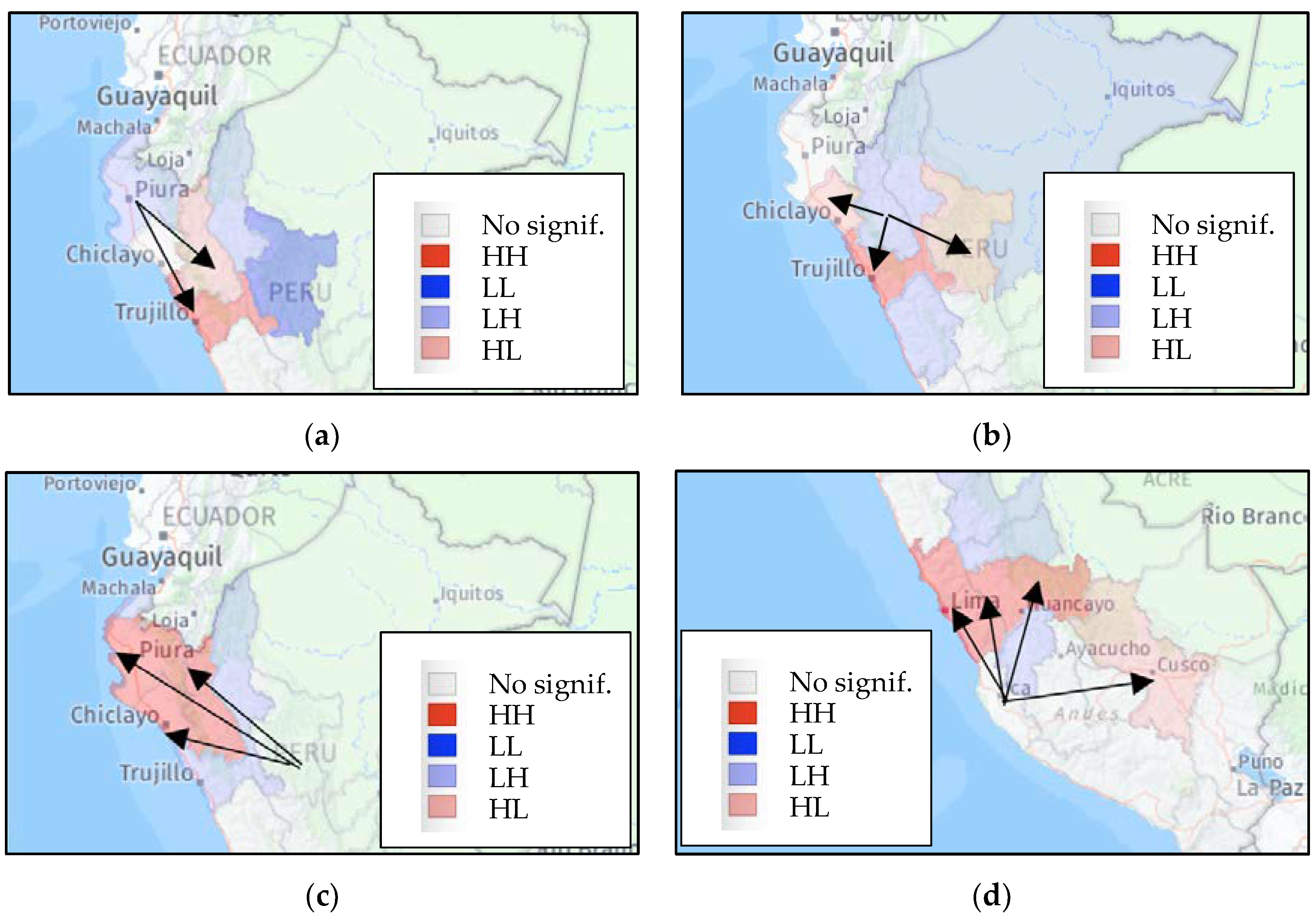
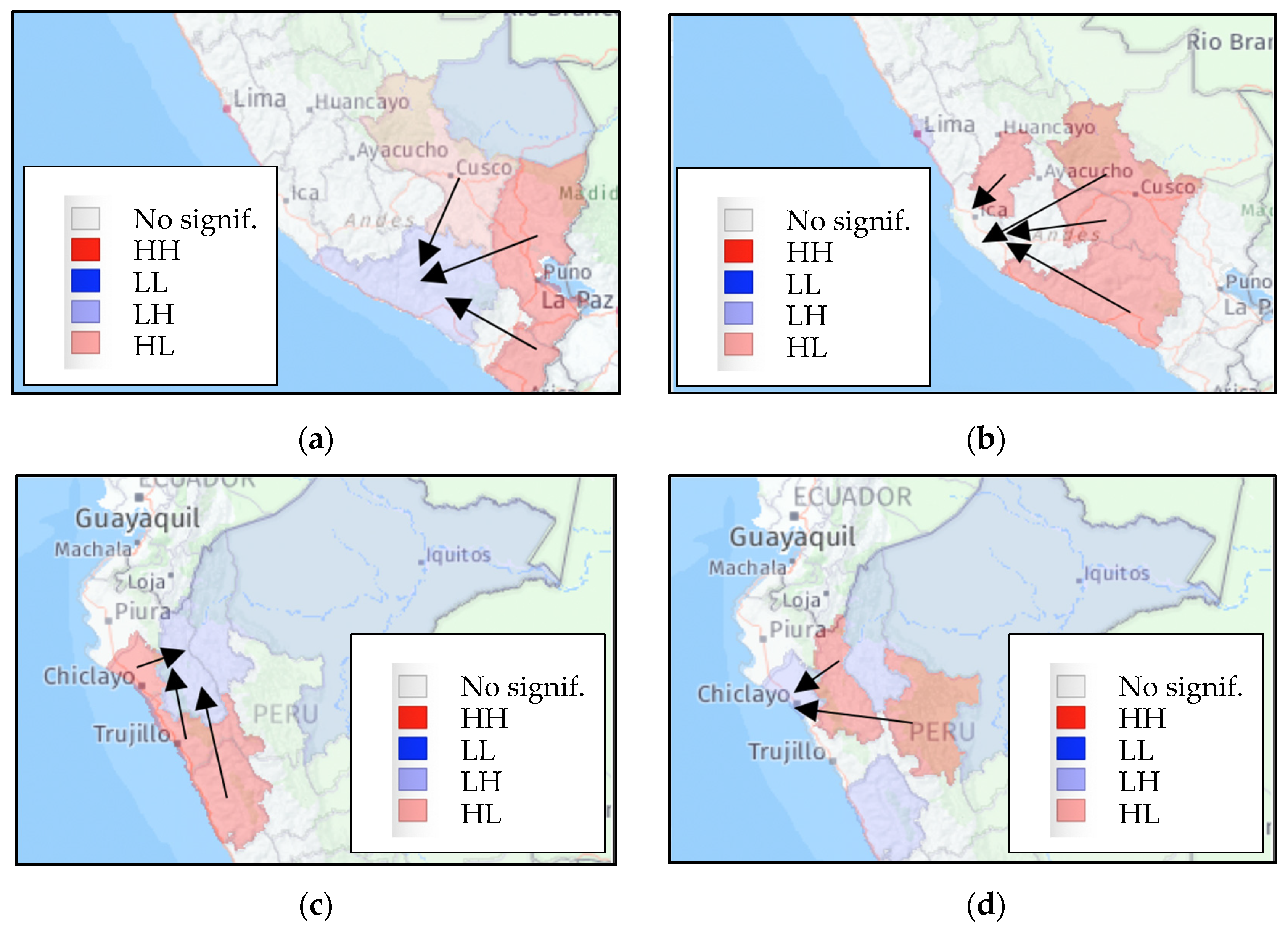
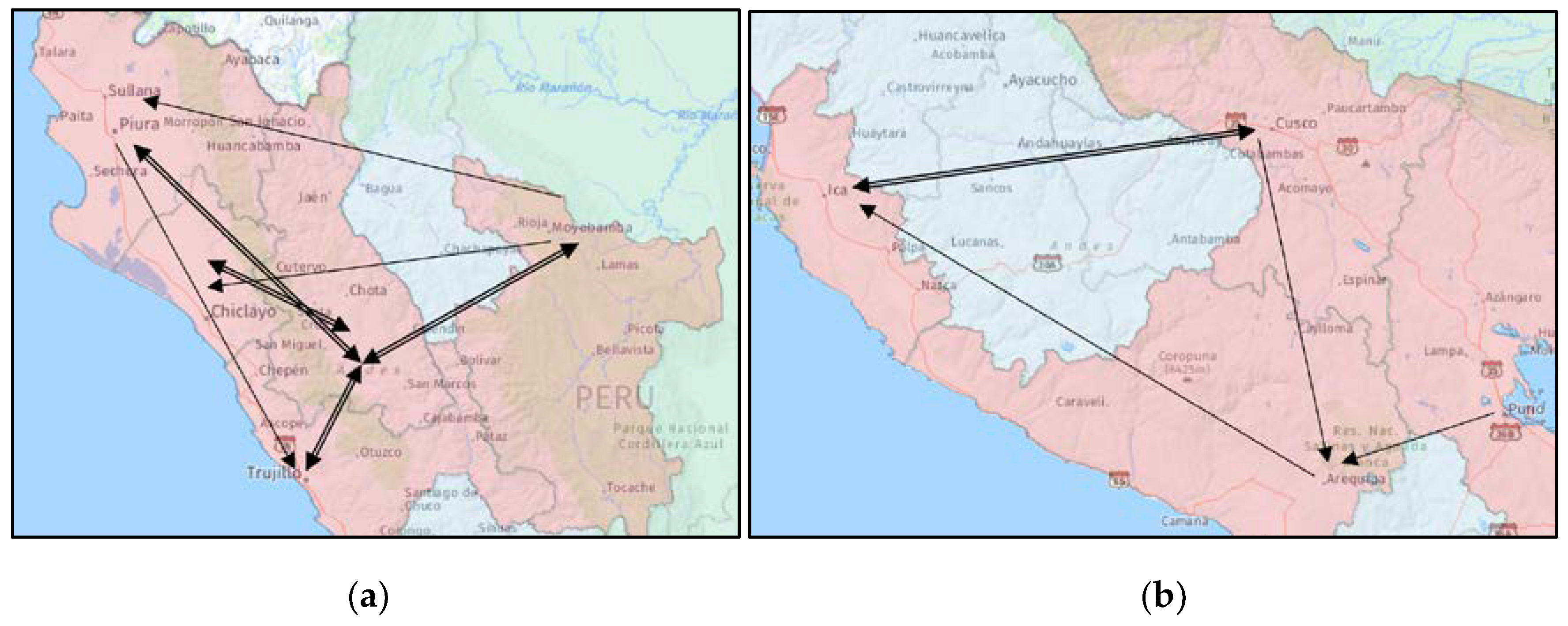
3.2.3. LISA Tests of Local Spatial Autocorrelation of Flows

The LISA tests of local spatial autocorrelation of flows detects those values of the quadrants of the Moran scatter diagrams with statistically significant values to identify hot spots, cold spots, and atypical agricultural trade flows at each origin and destination. As with the Moran’s I statistics, the LISA tests can be expressed in two ways. Equation (11) presents the test for the n variables τ_ID of agricultural transport costs from each origin region i to a specific destination D, which serves to detect the existence of clusters or spatial agglomerations in the vicinity of the origin regions that carry agricultural goods to a certain destination region. This statistic is called I_iD test of destinations:

$$I_{iD}=\frac{{\sum }_j{w}_{ij}{z}_{iD}·z_{jD}}{{\sum }_i{z}_{iD}^2/n},$$

(11)

In Equation (12), the test is presented for the n variables τ_Oj of agricultural transport cost from a given origin region O to all destination regions j. This test serves to detect the existence of clusters or spatial agglomerations in the vicinity of the destination regions that carry agricultural goods to a certain origin region. This statistic is called I_Oj test of origins:

$$I_{Oj}=\frac{{\sum }_j{w}_{ij}{z}_{iO}·z_{jO}}{{\sum }_i{z}_{iO}^2/n},$$

(12)

For the computation of the LISA test, we use the median instead of the mean to calculate the spatially lagged variables, as proposed in [18]. The LISA inferential process is similar to that followed for the global Moran index, except that in this case, the permutation is carried out for each and every one of the observations, obtaining a pseudo p-value for the total N² dyadic elements of Table 1, for $N=n\times n$ regions.

The calculations of the Moran I tests and the LISA tests for the origin and destination regions that are statistically significant are presented in

Table 2. Results of the Moran I and LISA tests for origin and destination regions.

Clusters in Origin Regions				Clusters in Destination Regions
Destination	Origin	Moran I	LISA	Origin	Destination	Moran I	LISA
Arequipa		0.272 ***		Cajamarca		0.184 ***
	Cusco		0.311 ***		La Libertad		0.518 ***
	Puno		0.331 ***		Lambayeque		0.664 ***
	Tacna		0.430 **		San Martín		0.175 ***
Cajamarca		0.224 ***		Ica		0.164 **
	Ancash		0.060 **		Cusco		0.163 ***
	La Libertad		0.258 ***		Junín		0.192 **
	Lambayeque		0.039 **		Lima		0.086 **
					MLC a		0.331 **
Ica		0.103 ***		Piura		0.122 **
	Apurímac		0.152 **		Cajamarca		0.013 **
	Arequipa		0.605 **		La Libertad		0.243 ***
	Cusco		0.008 **
	Huancavelica		0.233 **
Lambayeque		0.127 **		San Martín		0.129 **
	Cajamarca		0.351 ***		Cajamarca		0.354 **
	San Martín		0.168 **		Lambayeque		0.182 **
					Piura		0.447 **

*** and ** mean significant for p-value < 0.01 and a p-value < 0.05, respectively. ^a MLC corresponds to Metropolitan Lima and El Callao.

.

These results show the existence of both global and local positive spatial autocorrelation of agricultural trade flows at the Peruvian regional level. It means that nearby regions have similar agricultural trade flows, thus indicating spatial clustering. Figure 2 and Figure 3 graphically represent the results presented in Table 2. Both figures show that geographically close values of the agricultural trade flows tend to cluster with similar values of the variable in a map, i.e., high values tend to be located close to high values, and low values are located close to low values.

Figure 2a–d show the clusters formed in destination regions created by an origin region. We observe the conformation of three clusters in the north part of the country (Figure 2a–c) and one cluster in southern Peru (Figure 2d). The clusters originated by the regions of Piura, Cajamarca, and San Martín make up an agricultural cluster of intense commercial dynamism in northern Peru. These regions trade through the Fernando Belaunde Terry Highway, which connects the jungle regions (San Martín) with the coastal regions (Piura, La Libertad, and Lambayeque), passing through the Cajamarca region, located in the sierra of the country. The export agricultural products from these regions (cocoa and coffee, primarily) are concentrated in the Piura region, which houses the Port of Paita, the second busiest container port after the Port of El Callao, located in the MLC region. Figure 2d shows the cluster created by the Ica region in the southern part of the country. This region mainly supplies the regions of Cusco, Junín, Lima, and MLC (Metropolitan Lima and El Callao region) with avocados, asparagus, and grapes, part of the production of which is sent abroad through the Jorge Chávez International airport and Port of El Callao.

Figure 3a–d show the clusters in origin regions created by destination regions. These clusters are made up of regions that agglomerate to provide a particular region with agricultural goods and related services. This is the case of the regions of Puno, Tacna, and Cusco, which supply the Arequipa region with agricultural products such as coffee, quinoa, and olives, both for local consumption and for export through the Port of Matarani (Figure 3a). Other important cluster is found in the south-central part of the country (Figure 3b), where the regions of Arequipa, Cusco, Apurímac, and Huancavelica provide the region Ica with agricultural goods (onions, avocados, asparagus, paprika, and coffee), which are mostly concentrated for export through the Port of El Callao.

As shown in Figure 4a,b, agricultural trade flows create intense trade exchange networks both in two spatial clusters located in northern and southern Peru.

We can say that ESFDA results yield valuable insights about the clustering of agricultural trade flows that are suggestive of the diffusion of interregional trade. Certainly, the northern regions of the country (Figure 4a) have created a more intense spatial network for trade exchange of agricultural products than the southern regions (Figure 4b). This is mainly due to the influence exerted by the Port of Paita that operates as a centripetal force on agricultural export goods in the northern regions of the country. Our results are consistent with the findings of the World Bank [19] that identified six main agricultural export corridors in Peru, three of which have been detected by ESFDA methods.

These ESFDA tools detect the existence of significant global and local spatial autocorrelation in the distribution of agricultural transport flows. That is, agricultural trade flows are not randomly distributed among the Peruvian regions but spatially clustered. These detected spatial trends and clusters must be tested and, most probably, explicitly specified in econometric models of agricultural transport flows in Peru, since they are also relevant explanatory variables addressing this phenomenon.

4. Econometric Modelling

In this section, we present the econometric origin-destination flow models and the explanatory variables used to examine the effects of agricultural transport costs on the spatial organisation of regional structures in Peru. Origin-destination flow models, like the one set up in Equation (8), use agricultural trade flow data to explain spatial interactions from a set of origin locations to a set of destination locations in the geographic domain of Peru at the regional level (Supplementary Materials).

4.1. Non-Spatial Origin-Destination Model

The non-spatial version of origin-destination flow models assumes independence of flows and uses Ordinary Least Square (OLS) for its estimation. Taking into account Tanaka’s linear specification of the model of agricultural trade costs in Equation (8), this model can be formulated as follows:

$$y=X\beta +\epsilon ,$$

(13)

$$X\beta ={\alpha }_0{\iota }_N+X_o{\beta }_o+X_d{\beta }_d+{\alpha }_1{D}_{od}+{\alpha }_2{D}_{od}^2,$$

(14)

where y is an N by 1 vector of the natural log of agricultural trade flows (ATC, in Equation (8)); ${\iota }_N$ is an N by 1 vector of ones with α₀ representing a constant parameter term; $X_o{\beta }_o$ and $X_d{\beta }_d$ are respectively $X_o={\iota }_n\otimes X$ and $X_d={\iota }_n\otimes X$, where X is an n-by-n matrix of the natural log of independent variables for the n regions and $\otimes$ represents a Kronecker product, with ${\beta }_o$ and ${\beta }_d$ being their related scalar parameters; $D_{od}$ is an N by 1 vector of the natural log of distance between each o, d pair of regions with α₁ and α₂ being the associated scalar parameters, and ε is the N by error term vector which is assumed $\epsilon ~N\left(0,{\sigma }^2{I}_N\right)$, for ${\sigma }^2$ the constant variance of the error term and $I_N$ an identity matrix of order N.

The X matrix must contain the independent variables of the model, that is, the main determinants of agricultural trade flow variables. As stated in the literature, these are associated with the supply, demand, and efficiency sides of the economy. On the supply side, trade flow variations are directly proportional to the regional economic dynamics since a higher economic growth should lead to more trade in the agricultural sector because of a higher production of goods [20,21]. On the demand side, a price-demand relationship variable involves a negative relation between trade flows and prices of agricultural goods: an increase in prices for goods should reduce its demand, which in turn would lead to a reduction of agricultural trade flows [22,23]. Last, on the efficiency side, agricultural trade flows are directly proportional to the efficiency of road transport networks because a better-quality infrastructure should lead to more trade in both urban and agricultural areas [24,25].

Hence, the origin-destination model for agricultural trade flows of Peru includes three independent variables:

• Gross value added in each region, which measures regional economic dynamics. Since agricultural trade flows are directly proportional to the economic activity in regional economies, we would expect a positive relationship between these flows and the gross value added.
• Consumer price index variation for agricultural products in each region, which approximates the price-demand relationship of agricultural goods. Prices increment should reduce the demand for goods, and lead to reductions of agricultural trade flows, thus effects associated with change to consumer price index should be negative with respect to trade flows.
• Paved neighbourhood road length in each region measures road transport network efficiency. A better-quality infrastructure should lead to more trade, therefore, we would expect a positive relationship between trade flows and paved neighbourhood road length.

In addition, we use the distance and the squared distance between each pair of regions as extra explanatory variables to capture convexity-concavity patterns associated with real transportation data for agricultural goods. The summary statistics of dependent and independent variables of the origin-destination model are shown in

Table 3. Description of the dependent and independent variables.

Variable	Description	Units	Mean	Std	Min	Max
Dependent variable
Agricultural trade flows	Agricultural transport costs between each pair of regions. Authors calculations (see Section 3.2).	Dollar per ton/h	351,504.6	542,531.8	732.7	3,336,130.4
Independent variables
Regional economic dynamics	Gross value added in each region. National Institute of Statistics and Informatics (INEI)	(Index 2007 = 100)	137.3	20.6	89.0	189.8
Price-demand relationships	Consumer price index variation for agricultural goods in each region. INEI.	Consumer Price Index	2.8	1.3	0.4	5.7
Road transport network efficiency	Paved neighbourhood roads length in each region. Ministry of Transport and Communications (MTC).	km	77.6	94.1	66.2	403.3
Spatial variable	Distance between each pair of regions. Authors calculations based on data from INEI.	km	720.1	413.7	56.1	1948.9

.

The parameters of the non-spatial models are estimated by OLS (see the main results in

Table 4. Coefficient estimates for least-squares and spatial autoregressive models.

Variable		Least-Squares Model	Spatial Autoregressive
		Coefficient	Coefficient
Constant		−13.5381 *	−8.6443
βd	consumer price index for agricultural goods	−0.6002 **	−0.2285
βd	paved neighbourhood roads	0.6885 ***	0.3143 ***
βd	regional gross value added	3.5698 ***	1.4912
βo	consumer price index for agricultural goods	−0.3295	0.0579
βo	paved neighbourhood roads	0.1188	0.0653
βo	regional gross value added	0.0008	0.1286
log(distance)		−0.0085 ***	−0.0007
log(distance2)		0.30 × 10−5 ***	0.13 × 10−6
ρd			−0.1817 *
ρo			0.6435 ***
ρw			0.4874 ***

*** p-value < 0.01; ** p-value < 0.05; * p-value < 0.1.

). The R-squared statistic was 0.26, and the distance variable has a negative and significant coefficient, while the squared distance variable coefficient is positive, as expected. This last result implies that an increase in distance is associated with a decline in agricultural transport costs, a finding that is inconsistent with the strictly convex curve of the Krugman iceberg specification, as shown in Figure 5a.

However, as noted by many econometricians (e.g., [26,27]), the OLS estimation of the non-spatial origin-destination model is unsuitable for many spatial interaction phenomena (e.g., the agricultural transport flows), because it assumes independence among flows. Due to the fact that spatial interactions are operationalised through spatial autocorrelation in econometric models, if OLS is used in its presence, the resulting parameter estimates can suffer from potential bias and inefficiency [28].

4.2. Spatial Origin-Destination Model

4.2.1. Specification

LeSage and Pace extended the basic formulation of the origin-destination flow model to allow for spatial dependence by means of explicitly accounting for origin-based, destination-based, and origin-to-destination-based neighbourhood influences [26]. Origin-specific variables denote the ability of origin locations to create flows, whereas destination-specific variables represent the attraction of destination locations. Origin-destination functions in an agricultural setting indicate how agricultural trade interactions are obstructed by geographical dimensions.

Methodologically, origin-based, destination-based, and origin-to-destination-based neighbourhood influences are accounted for using the spatial weight matrices W_o, W_d, and W_w, respectively. Hence, the spatial autoregressive (SAR) interaction model of agricultural transport flows is expressed as follows:

$$y={\rho }_o{W}_{o}y+{\rho }_d{W}_{d}y+{\rho }_w{W}_{w}y+X\beta +\epsilon$$

(15)

$$X\beta ={\alpha }_0{\iota }_N+X_o{\beta }_o+X_d{\beta }_d+{\alpha }_1{D}_{od}+{\alpha }_2{D}_{od}^2 ,$$

(16)

The spatial origin-destination flow model comprises three N by 1 spatially lagged dependent variables of flows, which represent the strength of origin-based, destination-based, and origin-to-destination based spatial dependence each one with their scalar parameters ${\rho }_o,{\rho }_d,{\rho }_w$, correspondingly. In a previous paper, LeSage and Pace use the Kronecker product of the conventional spatial weight matrix (W) of order n by n, and an identity matrix (I_n) equal in size to that of the spatial weight matrix to describe spatial connectivity between the n regions [26]. The origin spatial weight matrix (W_o), the destination spatial weight matrix (W_d), and the origin-to-destination spatial weight matrix (W_w), are obtained, respectively, as follows:

$$\begin{gathered} W_o=W\otimes I_n \\ {W}_d=I_n\otimes W \\ {W}_w=W\otimes W \end{gathered}$$

(17)

The $W_o$ is an N-by-N row standardized spatial weight matrix used to capture origin-based spatial dependence, and analogously, $W_d$, is an N by N row standardized spatial weight matrix used to capture destination-based spatial dependence. Operationally, $W_{o}y$ and $W_{d}y$ reflect, respectively, the average of flows from neighbours of the origin to the destination and the average of flows from the origin to neighbours of the destination. Lastly, $W_w$, is an N-by-N row standardized spatial weight matrix defined as the product of $W_o$ and $W_d$, i.e., $W_w,=W_o·W_d$, which captures origin-to-destination spatial dependence and it represents the average of flows from neighbours of the origin to neighbours of the destination.

4.2.2. Estimation of the SAR Origin-Destination Model

LeSage and Pace propose estimating this SAR origin-destination model by Maximum Likelihood (ML) in [26] and in [27], they set forth a Bayesian Markov chain Monte Carlo (MCMC) approach to estimate the SAR model. We use the Bayesian MCMC to estimate the spatial autoregressive (SAR) interaction model of agricultural flows. Lower and upper 0.05 and 0.95 credible intervals are reported based on the retained 3000 Bayesian MCMC SAR draws. Bayesian MCMC SAR estimates were based on 5500 draws with 2500 omitted for start-up as defined in [29].

Estimates for the SAR interaction model are shown in Table 4. There is a high indication of origin- and origin-to-destination-based spatial dependence. These results confirm the effectiveness of the ESFDA for clusters in origin-regions. The coefficients ${\rho }_o$ and ${\rho }_w$ were 0.64, and 0.48, respectively, and the 99 percent credible intervals indicate they are different from zero. The destination-based spatial dependence captured by ${\rho }_d$ = −0.18 also was significant although proved to be the least influential for detecting spatial dependence patterns. The coefficient for the distance variable was significant and negative (−0.0007) and much closer to zero than the least-squares estimate (−0.0085), as shown in Figure 4. It is a usual result for the estimate on distance to fall in significance when spatially lagged variables are included into a SAR interaction model as distance operates as a proxy for spatial dependence when it is not incorporated [30,31].

5. Discussion on the Effect Estimates

5.1. Non-Spatial Origin-Destination Model

Effects estimates for the non-spatial and SAR interaction model are reported in

Table 5. Effect estimates for the least-squares and spatial autoregressive models.

Variables	Least-Squares Model			Spatial Autoregressive
	Mean	Median	Std. Dev.	Mean	Median	Std. Dev.
Origin-consumer price index for agricultural goods	0.0637	0.0614	0.3079	−0.1532	−0.1316	1.0399
Origin-paved neighbourhood roads	0.0595	0.0596	0.0956	0.5969	0.4749	0.7727
Origin-regional gross value added	0.1681	0.1422	1.0593	2.5751	2.0815	5.1307
Destination-consumer price index for agricultural goods	−0.2081	−0.2102	0.3007	-0.5848	−0.5369	1.1752
Destination-paved neighbourhood roads	0.2967	0.2960	0.1036	1.0031	0.8885	0.8138
Destination-regional gross value added	1.4238	1.4327	1.0543	4.6975	4.1212	5.5379
Intraregional-consumer price index for agricultural goods	−0.0060	−0.0060	0.0180	−0.0207	−0.0186	0.0564
Intraregional-paved neighbourhood roads	0.0148	0.0149	0.0059	0.0453	0.0409	0.0352
Intraregional-regional gross value added	0.0663	0.0661	0.0628	0.2052	0.1807	0.2516
Network-consumer price index for agricultural goods	--	--	--	−5.7770	−4.0858	19.0636
Network-paved neighbourhood roads	--	--	--	12.3269	9.3101	17.7252
Network-regional gross value added	--	--	--	56.3468	38.4989	109.0265
Total-consumer price index for agricultural goods	−0.1504	−0.1511	0.4493	−6.5357	−4.7502	21.1928
Total-paved neighbourhood roads	0.3711	0.3721	0.1471	13.9721	10.7266	19.3182
Total-regional gross value added	1.6582	1.6515	1.5710	63.8246	44.3224	119.5158

.

The non-spatial regression estimates indicate that a 1 percent increase in consumer price index for agricultural goods at the origin region would lead to a 0.06 percent increase in the agricultural trade flows while a 1 percent increase in paved neighbourhood roads at the origin region would lead to a 0.05 percent increase in trade flows in the agricultural sector. Both estimates are close to zero and thus proved to have little influence in the standard regression model. The impact of increasing regional gross value added at the origin and at the destination region by 1 percent would be to increase agricultural trade flows by 0.16 and 1.42 percent, respectively. Thus, supply factors influencing trade flow variations proved to be the most important in the non-spatial model.

The intraregional impacts of increasing consumer price index for agricultural goods, paved neighbourhood roads or regional gross value added in the representative region are small and correspond to −0.0060, 0.0148, and 0.0663, respectively. This suggests that increasing the conditions that generate transport cost variations in the Peruvian agricultural sector would lead to more trade within the region, limiting the emergence of external economies of scale across regions.

Total effects reflect the sum of the origin, destination, and intraregional impacts on agricultural trade flows in and out of regions as well as within regions arising from variations in the independent variables of the model. The total effect for consumer price index assessed by increasing consumer price index for agricultural goods by 1 percent is a decrease in agricultural trade flows (in and out of regions as well as within regions) by around 0.150 percent. The total effect of increasing regional gross value added and paved neighbourhood roads by 1 percent is a 1.6582 and a 0.3711 percent increase in agricultural trade flows (in and out of regions as well as within regions), correspondingly.

5.2. Spatial Origin-Destination Model

Agricultural trade flows exert different types of spatial interactions depending on the geographic domains in which they operate. Economic factors that lead to agricultural trade flows from any origin region to a specific destination may create analogous trade flows from neighbours of that origin to the same destination. Likewise, an analogous reasoning holds for destination-specific determinants that constitute a centripetal force for destination locations. Socio-economic influences that cause a destination region to import agricultural goods from a specific origin region may bring about the neighbours of that destination to import similar agricultural products from that origin. Origin-to-destination interactions among regions reflect the average of flows from neighbours of the origin region to neighbours of the destination region.

Spatial interactions in agricultural settings are approximated by the total effects of changes in geographical characteristics on agricultural trade flows in both origin and destination regions. Following [29], these total effects ($TE$) can be decomposed into four effects: origin effect ($OE$), destination effect ($DE$), intraregional effect ($IE$) and network effect ($NE$), which are estimated using a matrix of partial derivatives. For every of these four components ($OE$, $DE$, $IE$ and $NE$), we calculate similar scalar summary measures as for the $TE$, that quantifies the overall impacts of a change to the rth characteristic of all regions on origin-destination agricultural trade flows.

With respect to effect estimates for the SAR interaction model, we can see that the SAR interaction model attributes a greater impact to origin and destination effects generated by regional economic dynamics. We find that a 1 percent increase in gross value added produces a 2.57 and 4.69 percent increase, respectively, in agricultural trade flows both at origin and destination. Note that effect estimates show that destination-based dependence is more important than origin-based, and that OD-based dependence for interregional agricultural trade has a flow, which implies that destination explanatory variables exert trade flow attraction to destination locations.

Note that for origin effects, a 1 percent increase in consumer price index for agricultural goods leads to a 0.15 percent decrease in agricultural trade flows under SAR interaction models, while the same increment would lead to 0.06 percent increase in agricultural trade flows under the case of least-squares estimates. This contradictory result may be indicative of biased and inconsistent least-squares estimates in the presence of spatial dependence.

Intraregional effects were small but different from zero for the three explanatory variables under study. These results suggest that variations in the determinants of agricultural trade flows lead to more trade within the region, which would be an explanation of the low levels of trade across regions in Peru as reviewed in Section 3.1. Note that effect estimates for the three explanatory variables proved to be greater in the settings of the SAR interaction model than in the non-spatial model estimates, which is indicative of the relevance of spatial dependence in origin-destination flow models.

The great contribution of spatial interaction models resides in the quantification of network effects or spillover effects and in the contextually rich information it produces. Spillover effects are interpreted as changes at one point in time to the changes in flows agglomerated over the network required to reach a new steady-state equilibrium over all regions [29]. We find that a 1 percent increase in consumer price index for agricultural goods in the representative region would lead to a 5.77 percent (cumulative) decrease in agricultural trade flows throughout the network of regions. Likewise, the network effect for a 1 percent increase in paved neighbourhood roads in the traditional region leads to a 12.32 percent cumulative increase in agricultural trade flows throughout the region.

The spillover effects related to the diffusion of regional gross value added throughout the network of regions proved to be the most influential in the spatial origin-destination flow model. An increment of 1 percent in gross value added would lead to a 56.34 percent cumulative increase in agricultural trade flows across all regions. This result can be understood as the long-run increase generated by an increment of regional economic dynamics into agricultural trade flows cumulated over the network of 25 Peruvian regions. This cumulative effect over time would contribute to the configuration of a new steady-state equilibrium throughout the network of regions in Peru. Network externalities prove that flows are systematically associated with flows to or from nearby regions; thus, generating the emergence of spillover effects in the agricultural sector across Peruvian regions.

6. Conclusions

Most NEG models have approached agglomeration process by assuming free transport of the agricultural good. This assumption, however, involves the theoretical shortcoming that the agricultural sector must be sufficiently large for dispersion to occur as an equilibrium outcome, which impedes the examination of the spatial spillover effects in agricultural settings. To the best of our knowledge, the empirical implications of this theoretical flaw has not been addressed until now.

The issue is investigated in two dimensions. First, Krugman’s formulation of iceberg transport costs is reformulated to capture the agricultural transport costs. Second, ESDA methods and non-spatial and SAR interaction models are used to explore how the regional spatial structure changes when agricultural trade flows are included into the iceberg transport costs technology. The results of ESDA revealed the existence of agglomeration effects generated by agricultural transport costs, implying that prices of agricultural goods are concave with respect to distance. These results were confirmed by SAR interaction models, which support the notion that agricultural transport costs-created flows are associated with flows to or from neighbouring regions, causing the emergence of spatial spillovers across regions in Peru.

The results of the paper allow us to confirm McCann’s assertion [2] that Krugman’s formulation of iceberg transport costs acts as a break and counterweight to the emergence of agglomeration economies [32]. Our findings also support that NEG models have overshadowed the role of agricultural transport costs in determining the spatial distribution of economic activities [33], especially in developing countries like Peru where an important part of their inhabitants is devoted to agricultural activities.

The main policy implications of the paper are the importance of providing support for policy measures that facilitate the improvement of coordination mechanisms between agglomerations in agricultural and industrial environments, as shown in [34]. This has the following aims: removing coordination and cooperation failures by facilitating interlinkages and access to productive inputs; providing the availability of qualified labour; facilitating the presence of specialised service providers; and promoting an environment that allows the exchange and transfer of knowledge between economic agents. The implementation of these policies should help to reap the benefits from agglomeration.

As demonstrated in [35], the least productive entrepreneurs tend to agglomerate to the large core region as trade is liberalised, leading to sharply increasing regional income differences. Productive development policies (PDPs) emerge precisely to tackle this situation, addressing existing coordination failures, by promoting greater cooperation between economic agents—especially smaller firms with larger ones—in clusters or global value chains (GVC). PDPs also strengthen institutional governance mechanisms and implement instruments that promote interaction and efficiency within GVC.

In the specific context of Peru, it is necessary to reinforce the implementation of this type of policy through the deepening of three instruments: (i) supplier development programme to strengthen productive articulation and business networks [36] by improving the capabilities of supplier firms and their relationship with leading companies; (ii) cluster support programme to strengthen coordination and efficiency between firms in the same value chain, no matter the size, through the adoption of good production practices and product quality certification [37]; and (iii) executing a nuclei programme to promote the participation of micro and small firms in public purchases [38], seeking to generate conditions that enable a sustainable increase in their quality levels, productivity, and business formalisation.

The implementation of PDPs should be complemented by cross-cutting strategies to facilitate the needed enabling environment to institutionalise long-term business relationships between agglomerations in agricultural and industrial settings. A similar recommendation is also applicable to other countries with intense agricultural activity in which a phenomenon of agglomeration around agriculture could be occurring. The combined implementation of cross-cutting policies and PDPs might well contribute to closing technical-productive and quality gaps between agricultural and industrial areas and to the establishment of foundations for business internationalisation. These factors are relevant for the increase of value addition, productivity, competitiveness, and economic performance of these countries.

References

1. Krugman, P. Increasing returns and economic geography. J. Political Econ. 1991, 99, 483–499. [Google Scholar] [CrossRef]
2. McCann, P. Transport costs and new economic geography. J. Econ. Geogr. 2005, 5, 305–318. [Google Scholar] [CrossRef]
3. Fingleton, B.; McCann, P. Sinking the iceberg? On the treatment of transport costs in new economic geography. In New Directions in Economic Geography; Fingleton, B., Ed.; Edward Elgar: Cheltenham, UK, 2007; Chapter 6; pp. 168–203. [Google Scholar] [CrossRef]
4. Garretsen, H.; Martin, R. Rethinking (New) Economic Geography models: Taking geography and history more seriously. Spat. Econ. Anal. 2010, 5, 127–160. [Google Scholar] [CrossRef]
5. Samuelson, P.A. The transfer problem and transport costs, II: Analysis of effects of trade impediments. Econ. J. 1954, 64, 264–289. [Google Scholar] [CrossRef]
6. Fujita, M.; Krugman, P.R.; Venables, A.J. The Spatial Economy: Cities, Regions, and International Trade; MIT Press: Cambridge, MA, USA, 1999. [Google Scholar] [CrossRef]
7. Von Thünen, J.H. Der Isolierte Staat in Beziehung auf Nationalalo Konomie und Landwirtschaft; 1826 Reprinted by Fischer, G. Stuttgart; Pergamon Press: Oxford, UK, 1966. [Google Scholar]
8. Picard, P.M.; Zeng, D.-Z. Agricultural sector and industrial agglomeration. J. Dev. Econ. 2005, 77, 75–106. [Google Scholar] [CrossRef]
9. Tanaka, K. Transport Costs, Distance, and Time: Evidence from the Japanese Census of Logistics; IDE Discussion Papers; Institute of Developing Economies, Japan External Trade Organization: Chiba, Japan, 2010; Volume 241. [Google Scholar]
10. Evans, C.L.; Harrigan, J. Distance, time, and specialization: Lean retailing in general equilibrium. Am. Econ. Rev. 2005, 95, 292–313. [Google Scholar] [CrossRef]
11. Djankov, S.; Freund, C.; Pham, C.S. Trading on Time. Rev. Econ. Stat. 2010, 92, 166–173. [Google Scholar] [CrossRef]
12. IFPRI. Constructing a Typology of Rural Communities of the Peruvian Highlands Using Stochastic Profit Frontier Estimation; International Food Policy Research Institute: Washington, DC, USA, 2009. [Google Scholar]
13. Richards, P. It’s not just where you farm; it’s whether your neighbor does too. How agglomeration economies are shaping new agricultural landscapes. J. Econ. Geogr. 2018, 18, 87–110. [Google Scholar] [CrossRef]
14. Rangel-Preciado, J.; Parejo-Moruno, F.M.; Cruz-Hidalgo, E.; Castellano-Álvarez, F.J. Rural Districts and Business Agglomerations in Low-Density Business Environments. The Case of Extremadura (Spain). Land 2021, 10, 280. [Google Scholar] [CrossRef]
15. Läpple, D.; Renwick, A.; Cullinan, J.; Thorne, F. What drives innovation in the agricultural sector? A spatial analysis of knowledge spillovers. Land Use Policy 2016, 56, 238–250. [Google Scholar] [CrossRef]
16. Ranjan, P.; Tobias, J.L. Bayesian inference for the gravity model. J. Appl. Econom. 2007, 22, 817–838. [Google Scholar] [CrossRef]
17. Herrera-Catalán, P.; Chasco, C. Agglomeration on the periphery? Exploratory spatial analysis of agricultural transport flows in Peru. In Agglomeration Economies and Rural Development; Parejo-Moruno, F., Rangel-Preciado, J., Eds.; Dykinson Publishing: Madrid, Spain, in press.
18. Anselin, L. GeoDa Workbook. 2021. Available online: https://geodacenter.github.io/documentation.html (accessed on 14 November 2021).
19. World Bank. Peru—Towards a System Integrated City: A New Vision for Growth; World Bank Group: Washington, DC, USA, 2016. [Google Scholar]
20. Karp, L.S.; Perloff, J.M. A Synthesis of Agricultural Trade Economics. In Handbook of Agricultural Economics; Gardner, B.L., Rausser, G.C., Eds.; Elsevier: Amsterdam, The Netherlands, 2002; Chapter 37; pp. 3035–3213. [Google Scholar] [CrossRef]
21. Martin, W. Economic growth, convergence, and agricultural economics. Agric. Econ. 2019, 50, 7–27. [Google Scholar] [CrossRef] [Green Version]
22. McCalla, A.F. Impact of macroeconomic policies upon agricultural trade and international agricultural development. Am. J. Agric. Econ. 1982, 64, 861–868. [Google Scholar] [CrossRef]
23. Diaz-Bonilla, E.; Robinson, S. Macroeconomics, macrosectoral policies, and agriculture in developing countries. In Handbook of Agricultural Economics; Pingali, P., Evenson, R., Eds.; Academic Press: Burlington, ON, Canada, 2010; Chapter 61; pp. 3035–3213. [Google Scholar] [CrossRef]
24. Combes, P.-P.; Lafourcade, M. Transport costs: Measures, determinants, and regional policy implications for France. J. Econ. Geogr. 2005, 5, 319–349. [Google Scholar] [CrossRef]
25. Sotelo, S. Domestic Trade Frictions and Agriculture. J. Political Econ. 2020, 128, 2690–2738. [Google Scholar] [CrossRef] [Green Version]
26. LeSage, J.P.; Pace, R.K. Spatial econometrics modeling of Origin-Destination Flows. J. Reg. Sci. 2008, 48, 941–967. [Google Scholar] [CrossRef]
27. LeSage, J.P.; Pace, R.K. Introduction to Spatial Econometrics; CRC Press, Taylor & Francis Group: Boca Raton, FL, USA, 2009. [Google Scholar] [CrossRef] [Green Version]
28. Anselin, L. Spatial Econometrics: Methods and Models; Kluwer Academic Publishers: Amsterdam, The Netherlands, 1988. [Google Scholar] [CrossRef] [Green Version]
29. LeSage, J.P.; Thomas-Agnan, C. Interpreting spatial econometric origin-destination flow models. J. Reg. Sci. 2015, 55, 188–208. [Google Scholar] [CrossRef]
30. LeSage, J.P.; Fischer, M.M.; Scherngell, T. Knowledge spillovers across Europe, evidence from a poisson spatial interaction model with spatial effects. Pap. Reg. Sci. 2007, 86, 393–421. [Google Scholar] [CrossRef] [Green Version]
31. Sellner, R.; Fischer, M.M.; Koch, M. A spatial autoregressive Poisson gravity model. Geogr. Anal. 2013, 45, 180–200. [Google Scholar] [CrossRef] [Green Version]
32. Martínez-García, M.P.; Morales, J. Resource effect in the Core–Periphery model. Spat. Econ. Anal. 2019, 14, 339–360. [Google Scholar] [CrossRef]
33. Beghin, J.C.; Schweizer, H. Agricultural Trade Costs. Appl. Econ. Perspect. Policy 2021, 43, 500–530. [Google Scholar] [CrossRef]
34. Cai, J.; Li, X.; Liu, L.; Chen, Y.; Wang, X.; Lu, S. Coupling and coordinated development of new urbanization and agroecological environment in China. Sci. Total Environ. 2021, 776, 145837. [Google Scholar] [CrossRef] [PubMed]
35. Forslid, R.; Okubo, T. Agglomeration of low-productive entrepreneurs to large regions: A simple model. Spat. Econ. Anal. 2021, 16, 471–486. [Google Scholar] [CrossRef]
36. Liu, L.; Zhang, M.; Hendry, L.C.; Bu, M.; Wang, S. Supplier Development Practices for Sustainability: A Multi-Stakeholder Perspective. Bus. Strateg. Environ. 2018, 27, 100–116. [Google Scholar] [CrossRef] [Green Version]
37. Mishra, P.K.; Dey, K. Governance of agricultural value chains: Coordination, control and safeguarding. J. Rural Stud. 2018, 64, 135–147. [Google Scholar] [CrossRef]
38. Flynn, A. Investigating the implementation of SME-friendly policy in public procurement. Policy Stud. UK 2018, 39, 422–443. [Google Scholar] [CrossRef] [Green Version]
Figure 1. Peru: agricultural trade flows in 2013.
Land 11 00058 g001
Figure 2. Clusters in destination regions created by origin regions: (a) Origin: Piura; (b) Origin: Cajamarca; (c) Origin: San Martín; (d) Origin: Ica.
Land 11 00058 g002
Figure 3. Clusters in origin regions created by destination regions: (a) Destination: Arequipa; (b) Destination: Ica; (c) Destination: Cajamarca; (d) Destination: Lambayeque.
Land 11 00058 g003
Figure 4. Origin-destination transaction networks for agricultural goods; (a) North network; (b) South-Central network.
Land 11 00058 g004
Figure 5. Estimation of the effect of distance on agricultural transport costs.
Land 11 00058 g005