Analysis of the Spatiotemporal Heterogeneity of Various Landscape Processes and Their Driving Factors Based on the OPGD Model for the Jiaozhou Bay Coast Zone, China

Abstract

To date, various studies have analyzed changes in the landscape but there are few studies which have explored landscape processes and the corresponding driving factors. This study makes up for this deficiency in the systematic theoretical exposition and the spatiotemporal analysis of landscape processes. The results show that the amount of arable land outflow and built-up land inflow have resulted in an increase of 92,311.11 ha of built-up land that is mostly distributed around the administrative center and along the coast of Jiaozhou Bay. The outflow of ecological land is a major resource for replenishing arable land, by 37,016.19 ha, especially in terms of the grassland that is distributed in the hilly areas west of Jiaozhou Bay. The outflow of the salt-field, fish-farm and ecological land outflow have good connectivity, a large patch size, and an irregular shape. The ecological type, elevation, slope, and vegetation coverage are the four factors that have a great influence on all landscape processes. A gentler slope and lower elevation, and proximity to cities and towns land will produce more arable land outflow and built-up land inflow. However, arable land inflow and ecological land outflow are the opposite. This research will guide natural resource management for a rapidly developing coastal zone.

1. Introduction

“Landscape” refers to an area, as perceived by people, the character of which results from the action and interaction of natural and/or human factors [1]. The understanding of the landscape emerges as a complex of perceived characteristic areas that are formed by natural factors and human activity. Current developments in remote sensing and geo-information technologies facilitate the analysis of landscape patterns and their processes. Landscape patterns and landscape change, at all scales, have been extensively analyzed [2]. However, the processes of landscape change have rarely been the subject of current research. In this paper, we will take the discourse of “landscape processes” as the main outline to expand the discussion of the article. “Pattern”, “scale”, and “process” are important concepts in landscape ecology. However, the theoretical explanation of the “process” is somewhat insufficient, with most studies paying close attention to the ecological processes [2,3]. Landscape pattern analysis should develop from the current description of the static pattern to a dynamic pattern and link the pattern and process together [4]. Studies on the landscape change trajectory analysis (LCTA) have provided this chance. LCTA is an approach that is used for calculating the relationship between present-day landscape patterns, their attached values, and the past [5,6]. Landscape change trajectory forms a dynamic landscape type that includes temporal and spatial features and reflects the landscape process in space. It connects different temporal scales and spatial patterns.

It is a common research paradigm to analyze a landscape trajectory area and its landscape pattern index based on remote sensing image data [7,8,9,10]. Some studies have explored the trajectory of the change in the landscape index corresponding to different types of land cover [11]. A few scholars have used the Moran index and local indicator of spatial association (LISA) to analyze the spatial autocorrelation and heterogeneity of an ecological landscape loss trajectory [12]. Regression analysis is used for exploring the driving force mechanism. Based on regression analysis, some studies have explored the relationship between landscape trajectories and physical geographic features or socioeconomic factors [6,13,14]. At present, the methods used for exploring the forces that drive changes in the landscape are relatively simple, and mainly use empirical analysis methods or logistics regression analysis methods. Most research has been focused on the outcomes of landscape changes rather than the processes [5,6,15,16,17,18,19].

Spatial heterogeneity is a major feature of ecological and geographical phenomena. It refers to the uneven distribution of various geospatial attributes within a certain geographical area, or, simply, spatial variation of attributes [20]. Spatial heterogeneity with local clusters is a popular approach that explores, spatially, local clustering regions with similarities in their geographical attributes. It has been addressed by hundreds of quantitative measures in landscape geometry, LISA, Getis-Ord Gi [21,22,23], and geographically weighted regression (GWR). However, the geographical detector model can quantify the spatial stratified heterogeneity, which compares the spatial variance within a stratum and that between different strata [24,25]. The main idea of geographical detectors is that the study space is divided into subregions by variables, and the spatial variance within each subregion and among different subregions are compared to evaluate the determinant power of the potential explanatory variables. From 2010 to 2019, more than 100 research papers have been published using this model. The applications of the model are predominant in geographically local determinants or exploration of factors, spatial patterns, and investigation of heterogeneity [26]. The general geographical detectors include four parts, where the core part is the factor detector that quantifies the relative importance of different geographical variables. The other three parts are the interaction detector, risk detector, and ecological detector [26,27]. On 27 April 2021, the optimal parameters-based geographical detectors (OPGD) model was launched on the R “GD” package [28], which can choose the optimal partitioning method and quantity. This improves the operation magnitude of the geographical detector model and is not limited to the maximum number of lines, i.e., 32,769, in Excel.

The bay area usually has better living conditions, industrial production conditions, and, thus, the gulf area is usually highly developed. The Jiaozhou Bay coastal zone is a typical area, and its landscape has changed greatly since the reform and opening up occurred in 1978. Therefore, this area is extremely rich in spatial and temporal characteristics of landscape processes and is of high research value. Furthermore, exploring landscape processes in the Jiaozhou Bay coastal zone helps us to understand the changing mechanism of the coastal landscape in the typical bay area of China and provides policy suggestions for land management and control in the highly developed coastal zone.

The present study seeks to: (1) explain the connotation of the landscape processes and the possible drivers and driving mechanisms, (2) analyze the spatiotemporal heterogeneity of various landscape processes within the last 30 years in the coastal zone of the Jiaozhou Bay, and (3) explore the driving factors for the various landscape processes using the OPGD model. Finally, a few policy suggestions have been put forth for landscape process control in the Jiaozhou Bay coastal zone.

2. Materials and Methods

2.1. Theoretical Principle

Landscape processes are spatiotemporal changes in the landscape that can be perceived, and this perception can be visual or detected in remote sensing images. In maps and remote sensing images, a landscape process is a process of transforming one landscape type into another at different time and space scales and implies a change in the basic attributes of a landscape (Figure 1). A landscape process in a region might contain many microcosmic fragments in space and time. This process can also be measured using tools for the analysis of spatiotemporal heterogeneity. However, such a dynamic landscape process pattern is bound to be a pattern interwoven with different times and spaces.

The driving factors for a landscape process include human beings exploiting the natural space, building construction on cultivated land, and other ways of moving the landscape types toward more artificial types. On the contrary, it might also include human beings creating natural habitats, natural succession and disaster damage, returning farmland to forest land, grassland, or wetland, and other ways for transforming landscape types to more natural landscape types. The visual expression of a landscape process in space presents a shift in the landscape type and the landscape trajectory. Administrative intervention and planning control are common landscape process management methods.

2.2. The Study Area

The research area used in this study is located on the south bank of the Shandong Peninsula, near the South Yellow Sea, and has a slightly fan-shaped distribution around the semi-closed Jiaozhou Bay. The research area consists of eight districts, namely, Huangdao, Jiaozhou, Chengyang, Jimo, Laoshan, Shibei, and Shinan District (Figure 2). The Dagu, Xiaogu, Taoyuan, Moshui, Baisha, and Yanghe rivers flow through this area, and large amounts of sediment carried by the rivers form a tidal flat in the northern part of Jiaozhou Bay. The vegetation type groups of forests in the study area are deciduous broad-leaved forest, including Quercus, Acer, Pistacia chinensis, etc. The highest point is Laoshan Mountain, with an elevation of 1091 m.

The study area had a permanent resident population of 7,250,900 million as of the end of 2018, accounting for 77.18% of the total population of Qingdao, and produced a gross domestic product (GDP) of 104.0709 billion Chinese yuan. Many national development zones are located within this study area. For instance, the Huangdao economic development zone, the Hongdao high-tech zone, the west coast new development zone, and the Jiaozhou airport economic zone are located here (Figure 2). The study area has a high development intensity and is a typical coastal zone with a high opening intensity.

2.3. Data Source and Processing

The 30 m × 30 m grid land considered the data of eight county-level districts in Qingdao from 1990, 2000, 2010, and 2018, which were obtained from the Natural Resources and Environmental Sciences Data of the Chinese Academy of Science [29]. The geographical data has data integrity, and the comprehensive accuracy is close to 90% [30].

In this study, the salt-field and fish-farm landscape types were extracted by masking based on the land-use status maps and Google Earth satellite images for different years, which were independently extracted as code 5 mentioned above. The marsh in the unused land was classified into wetland and waters, and the rest were merged according to the first-level class. Then, the CNLUCC (dataset of land use and cover in China) classification system was redivided into arable land, woodland, grassland, wetlands and waters, salt-field and fish-farm, built-up land, and unused land. The spatial database of the different landscape types in the study area was formatted, and their codes were set as 1, 2, 3, 4, 5, 6, and 7, and are listed in

Table 1. Reclassification of the landscape types based on the CNLUCC.

The First-Level Type		The Secondary-Level Type	Reclassification Type
1	Arable land	11, 12	1	Arable land
2	Woodland	21, 22, 23	2	Woodland
		24	1	Arable land
3	Grassland	31, 32, 33	3	Grassland
4	Water area	41, 42, 43, 44, 45, 46	4	Wetlands and Waters
5	Urban and rural residential land/industrial land	51, 52, 53	6	Built-up land
6	Unused land	61, 62, 63, 65, 66, 67	7	Unused land
		64	4	Wetlands and Waters
99	Ocean	99	4	Wetlands and Waters

.

The driving factors selected in this study are as follows (

Table 2. Data source and format of driving force analysis.

Number	Data Description	Data Source/Format 2	The Data Unit
X1	Distance from the mean center of the development zone	Google maps	Meter
X2	Distance from rivers and lakes	www.openstreetmap.org	Meter
X3	Distance from shore (coastal administrative boundary)	www.resdc.cn	Meter
X4	Distance from cities and town land	The 30 m × 30 m grid of the CNLUCC data	Meter
X5	Slope	The 30 m × 30 m grid of ASTER GDEM V3	Percent
X6	Elevation	The 30 m × 30 m grid of ASTER GDEM V3	Meter
X7	NDVI 1 in October 1998	www.resdc.cn	No units of measure
X8	GDP in 1995	www.resdc.cn	Ten thousand yuan per square kilometer
X9	Population difference between 1995 and 2015	The 1 km × 1 km grid/www.resdc.cn	People per square kilometer
X10	Type of ecological land	The 30 m × 30 m grid of the CNLUCC dataset	21, 22, 23, 31, 32, 33, 41, 42, 43, 45, 45, 46 on CNLUCC dataset
X11	Growth of fixed investment	www.shujuku.org	Ten thousand yuan
X12	The density of road network	www.openstreetmap.org	Kilometer per square kilometer

¹ Normalized Difference Vegetation Index. ² Accessed on 18 December 2021.

). Most of the data in the following table have been clipped. For distance factors, the Generate Near Table in ArcGIS10.3 Tool was used. For the other factors, the sampling tool in ArcGIS10.3 was used. The relevant data were then linked in a table for the relevant spatial heterogeneity analysis.

In this study, the landscape processes with a conversion area ratio of >1% were regarded as the main landscape processes, and those with an area ratio of <1% were ignored. In the analysis of the spatial autocorrelation and the driving force analysis, fish spots of 200 m × 200 m were used as the basic unit for extracting the driving factor values and analyzing the spatial heterogeneity. The attribute values of the landscape processes belonging to this type were set to 1, whereas those not belonging to this type were set to 0.

2.4. The Research Methods

2.4.1. Spatiotemporal Characteristics for Analyzing the Landscape Processes

(1) Dynamic attitude

The dynamic attitude of a single landscape type can be used for representing the quantitative degree of change in the study area within a time range. The comprehensive dynamic attitude of the landscape types is integrated, and the transfer between the landscape types is taken into full consideration to describe the overall intensity of change in the regional landscape type [31].

(2) Transfer matrix and landscape trajectory

In this study, a transfer matrix has been used for analyzing the landscape processes in each decade from 1990 to 2018. The two maps corresponding to the two years were intersected and merged using ArcGIS10.3.

The landscape trajectory values can be expressed by the formula:

$$\begin{array}{c}CT={10}^{n-1}{P}_1+{10}^{n-2}{P}_2+\cdots +{10}^{n-i}{P}_i+\cdots +P_n\end{array}$$

(1)

where CT represents the trajectory codes on each grid in the research time sequence, $n$ represents the time node in the research time sequence number ($n$ > 1), and $P_i$ represents the raster data of the landscape type at the $i$th time node.

2.4.2. Exploring the Spatial Heterogeneity of Each Landscape Process

(1) Landscape pattern index

The landscape pattern index was calculated using the Fragstats4.2 software. The following landscape pattern indices were selected for the landscape pattern analysis, including the number of patches (NP), the landscape shape index (LSI), area (AREA_MN), fractal dimension index (FRAC_MN), aggregation index (AI), contagion index (CONTIG_MN), and shape index (SHAPE_MN). These indices are correlated with the degree of fragmentation, regularity, connectivity of the landscape type, and the degree of human disturbance, respectively [32,33].

(2) Global autocorrelation and LISA

Global spatial autocorrelation was used for testing the distribution pattern of an element in the entire space, which can be divided into aggregation, discrete, and random. In this study, the global Moran index was used for reflecting the spatial correlation of different landscape processes in the study area [34]. This method is well known in the research field and will not be elaborated.

Local spatial autocorrelation involves the decomposition of the global spatial autocorrelation into each spatial unit. It reflects the spatial correlation between the attribute value of the elements and the adjacent elements in the entire area and a small local area [20]. It is expressed as follows:

$$\begin{array}{c}\begin{array}{l}{\mathrm{LISA}}_i=\left(\frac{x_i-x}{S^2}\right)\underset{j=1}{\overset{n}{\Sigma }}{W}_{ij}\left(x_i-\overline{x}\right),i\ne j\\ S^2=\frac{1}{n}\underset{j=1}{\overset{n}{\Sigma }}{\left(x_i-\overline{x}\right)}^2,\overline{x}=\frac{1}{n}\underset{j=1}{\overset{n}{\Sigma }}{x}_i\end{array}\end{array}$$

(2)

where$S^2$ is the variance, $W_{ij}$ is the element of the spatial weight matrix, and $x_i$, $x_j$ are the spatial units after row standardization. The range of the Moran index value of the local units is [−1, 1]. According to the positive and negative ${\mathrm{LISA}}_i$ values, the spatial units can be divided into two types (namely, high-high and low-low), two types of positive correlation (namely, high-low and low-high), two types of negative correlation, and five types of insignificant correlation.

2.4.3. Analyzing the Driving Factors of the Landscape Processes: The OPGD Model in the R“GD” Package

The OPGD model includes five parts: factor detector, parameter optimization, interaction detector, risk detector, and ecological detector.

(1) Q-statistic

As the core part of the geographical detector, the factor detector reveals the relative importance of the explanatory variables with a Q-statistic. The Q-statistic compares the dispersion variances between observations in the entire study area and the strata of variables [24,25]. The Q-statistic is computed as follows:

$$\begin{array}{c}{Q}_v=1-\frac{{\Sigma }_{j=1}^M\left(N_{v,j}-1\right){\sigma }_{v,j}^2}{\left(N_v-1\right){\sigma }_v^2}\end{array}$$

(3)

where $N_{v,j}$and ${\sigma }_v^2$are the number of observations and their variance, respectively, within the entire study area, and$N_{v,j}$and${\sigma }_{v,j}^2$ are the number of observations and their variance, respectively, within the $j$th$\left(j=1,\dots ,M\right)$ subregion of the variable$v$. A large Q-statistic value implies the relatively high importance of the explanatory variable due to a large variance between the subregions.

(2) Interaction Q-statistic

The interaction detector determines the interactive impact of two overlapped spatial variables based on the relative importance of the interactions computed with the Q-statistic of the factor detector. The interaction detector explores an interaction by comparing the Q-statistic of the interaction with the two single variables. The interaction detector explores five interaction situations, including nonlinear weakening, univariable weakening, bivariable enhancement, independent, and nonlinear enhancement, as listed in

Table 3. Interactions between the two explanatory variables and their interactive impact.

Geographical Interaction Relationship	Interaction
$Q_{u{{\displaystyle \cup }}^{}v}<min\left(Q_u,Q_v\right){ }^1$	Nonlinear weakening: Impacts of single variables are nonlinearly weakened by the interaction of two variables.
$min\left(Q_u,Q_v\right)\le Q_{u{{\displaystyle \cap }}^{}v}\le max\left(Q_u,Q_v\right)$	Univariable weakening: Impacts of single variables are univariable weakened by the interaction.
$max\left(Q_u,Q_v\right)<Q_{u{{\displaystyle \cap }}^{}v}<\left(Q_u+Q_v\right)$	Bivariable enhancement: Impact of single variables are bi-variable enhanced by the interaction
$Q_{u{{\displaystyle \cap }}^{}v}=\left(Q_u+Q_v\right)$	Independent: Impacts of variables are independent.
$Q_{u{{\displaystyle \cap }}^{}v}>\left(Q_u+Q_v\right)$	Nonlinear enhancement: Impacts of variables are nonlinearly enhanced

¹ $Q_u$ is the Q-statistic of the variable $u$, $Q_v$ is the Q-statistic of the variable $v$, and $Q_{u{{\displaystyle \cap }}^{}v}$ is the Interact Q-statistic between the variables $u$ and $v$.

[24,25].

(3) The risk mean in the OPGD model

The risk mean is the mean statistic of the dependent variable attributes in different intervals of optimization of spatial discretization measured by the risk detector [26,28]. It can reflect the mean value of the dependent variable within the optimal interval and provide a basis for analyzing spatial heterogeneity.

3. Results

3.1. Overall Influence of the Landscape Process on the Quantity and Space of Different Landscape Types

3.1.1. The General Quantity and Distribution of the Different Landscape Types in Each Decade

The number of landscape types in the study area in each decade is shown in

Table 4. The number of landscape types in each decade.

Landscape Types	1990a		2000a		2010a		2018a
	Area/ha	Proportion	Area/ha	Proportion	Area/ha	Proportion	Area/ha	Proportion
1	393,809.58	61.93%	383,685.39	60.33%	387,605.25	60.73%	361,905.21	56.49%
2	48,124.35	7.57%	48,123.9	7.57%	41,474.61	6.50%	43,127.46	6.73%
3	65,403.36	10.29%	65,205.81	10.25%	19,870.92	3.11%	25,958.16	4.05%
4	25,633.08	4.03%	26,693.28	4.20%	27,732.06	4.35%	28,165.14	4.40%
5	26,351.37	4.14%	26,791.02	4.21%	20,321.28	3.18%	13,326.12	2.08%
6	75,513.78	11.88%	84,483.36	13.28%	140,744.79	22.05%	167,824.89	26.19%
7	1017.9	0.16%	1018.08	0.16%	456.93	0.07%	375.66	0.06%
Total area	635,853.42		636,000.84		638,205.84		640,682.64

. It can be seen that arable land, woodland, grassland, and built-up land are the main landscape types, which account for more than 90% of the total area of the region.

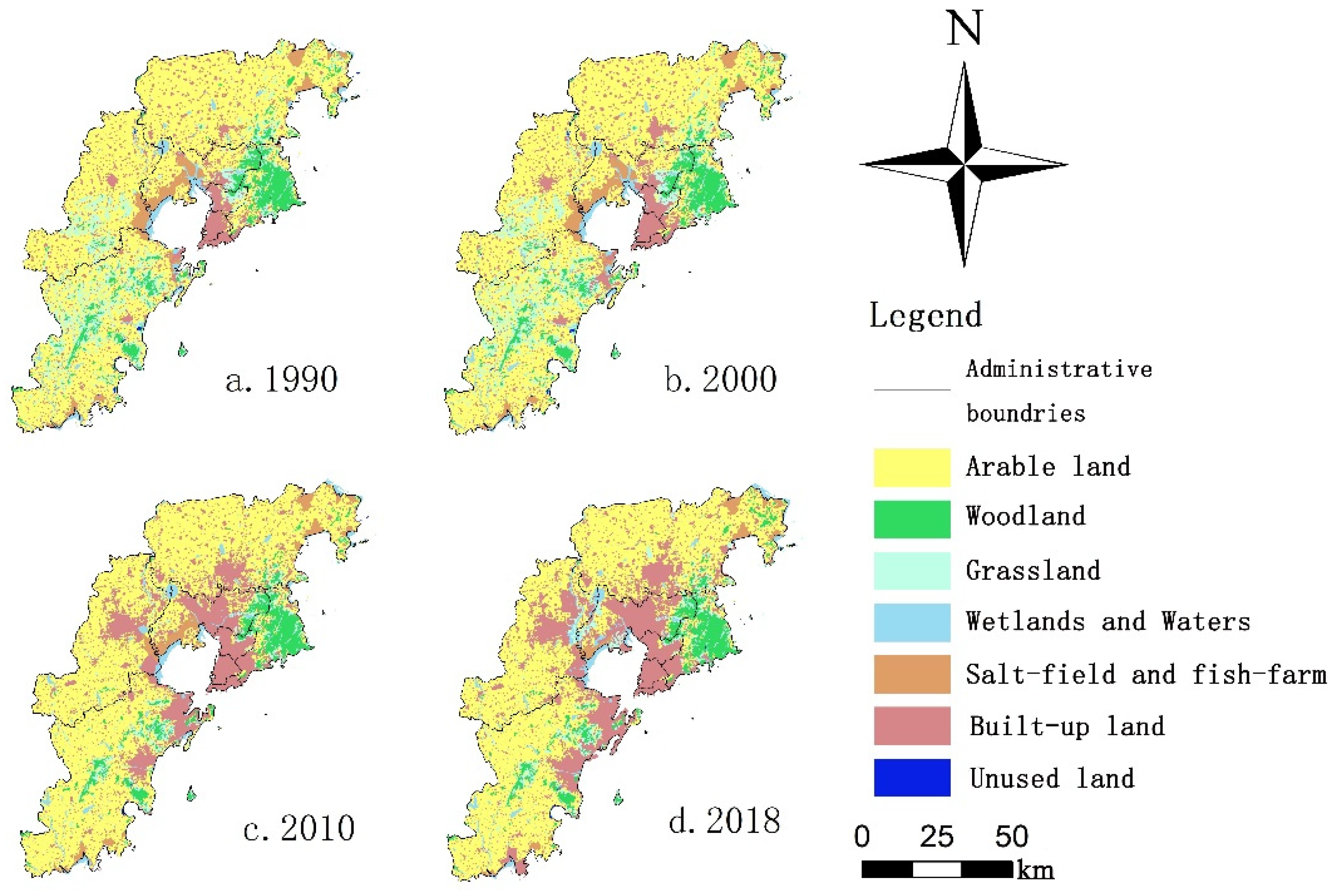
Arable land has always occupied the dominant position, from 1990 to 2018, spread over Jiaozhou District, Chengyang District, Jimo District, and Huangdao District. Woodland and grassland are mainly distributed in higher elevations of hills and mountains in Laoshan District, southern Jiaozhou district, and central Huangdao District. The wetlands and waters in the study area are mainly distributed in the north of Jiaozhou Bay, at the junction boundary of the administrative area of Jiaozhou District, Chengyang District, and Jimo district. The built-up land is located in the administrative center and around the bay (Figure 3).

3.1.2. Influence of the Landscape Process on the Quantity and Distribution of Different Landscape Types

In the study period, the arable land, woodland, grassland, and unused land exhibited an overall shrinking trend, whereas a gradual expansion of the built-up land was observed.

In the past 30 years, the arable land area decreased slightly, from 393,809.58 ha in 1990 to 361,905.21 ha in 2018, representing an overall proportion decrease of 5.45%. The period from 2010 to 2018 saw a loss of 25,700.04 ha of arable land. From 2000 to 2010, the area of woodland decreased significantly, by an amount of 6649.29 ha. In the next decade, the area of woodland rose slightly. The grassland area was stable from 1990 to 2000. However, it decreased sharply from 65,205.81 ha to 19,870.92 ha in 2000 and 2010, respectively, with a decrease rate of nearly 70%. The grassland area recovered slightly from 2010 to 2018.

The total amount of built-up land expanded from 75,513.78 ha in 1990 to 167,824.89 ha in 2018. The proportion of the regional area expanded from 11.88% in 1990 to 26.19% in 2018. The total area of built-up land increased from 84,483.36 ha between 2000 to 2010. In the past 30 years, the salt-field and fish-farm have reduced from 26,351.37 ha in 1990 to 13,326.12 ha in 2018, with the total area reduced by nearly half. The unused land has decreased by half, and the wetland water area has increased steadily. Wetlands and waters have increased slightly from 25,633.08 ha in 1990 to 28,165.14 ha.

As can be seen from Figure 3, arable land was occupied by the expanding rural and urban construction land, showing the characteristics of spatial fragmentation and shrinkage. Most of Chengyang District, the middle of Jiaozhou district, and the northwest of Huangdao District were occupied by built-up land. The spatial characteristics of and the grassland occupied by arable land are significant and are mainly concentrated in the south of Huangdao District and Jiaozhou district. Nevertheless, the spatial status of woodland and grassland in the eastern part of Chengyang District and Laoshan District were efficiently maintained. Wetlands and waters in the north of Jiaozhou Bay were increasingly occupied by the expansion of the built-up land. Salt-field and fish-farm areas were shrinking, especially in the north of Jiaozhou Bay, and large parts of them were turned into built-up land.

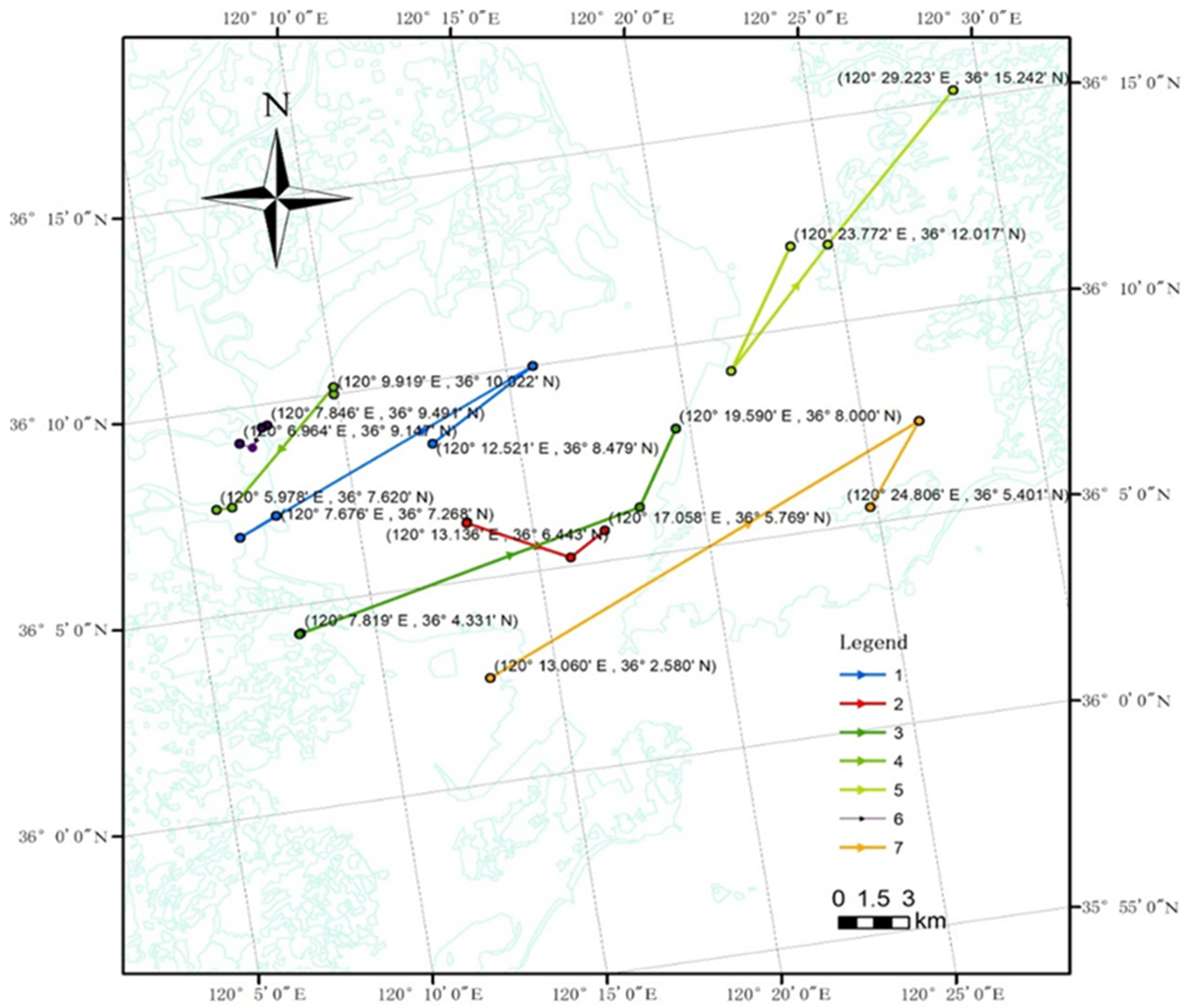
As can be seen in Figure 4, the mean centers generated by ArcGIS 10.3 of all landscape types showed a large migration distance between 2000 and 2010, except for salt-field and fish-farm areas. This indicates that the landscape process was very dramatic between 2000 and 2010.

The mean center of arable land and unused land moved to the northeast from 1990 to 2010 and folded back to the southwest. Combined with the quantitative and distribution characteristics of the above analysis, we found that the net area reduction in the southwest of the mean center was more than that in the northeast. It might be influenced by the landscape process of unbalanced inflow and outflow of the arable land or the unused land.

The mean centers of the grassland and the woodland migrated eastward on the whole. Combined with the above analysis, it can be observed that the woodland and the grassland being present in the eastern hilly region affected the shift of the mean center. The largest migration of the mean center was that of the grassland. It migrated 9480.334 m (3.669′) to the north and 16,083.74 m (11.746′) to the east in general.

The mean center of the wetlands and waters and the built-up land migrated to the southwest. The built-up land increased considerably, but the mean center of the construction land migrated slightly to the southwest. It moved by a smaller distance of 838.615 m to the south and 1186.41 m to the west.

3.2. Quantity and Spatial Distribution of Landscape Processes in Each Decade

3.2.1. Rate of Change of the Various Landscape Processes

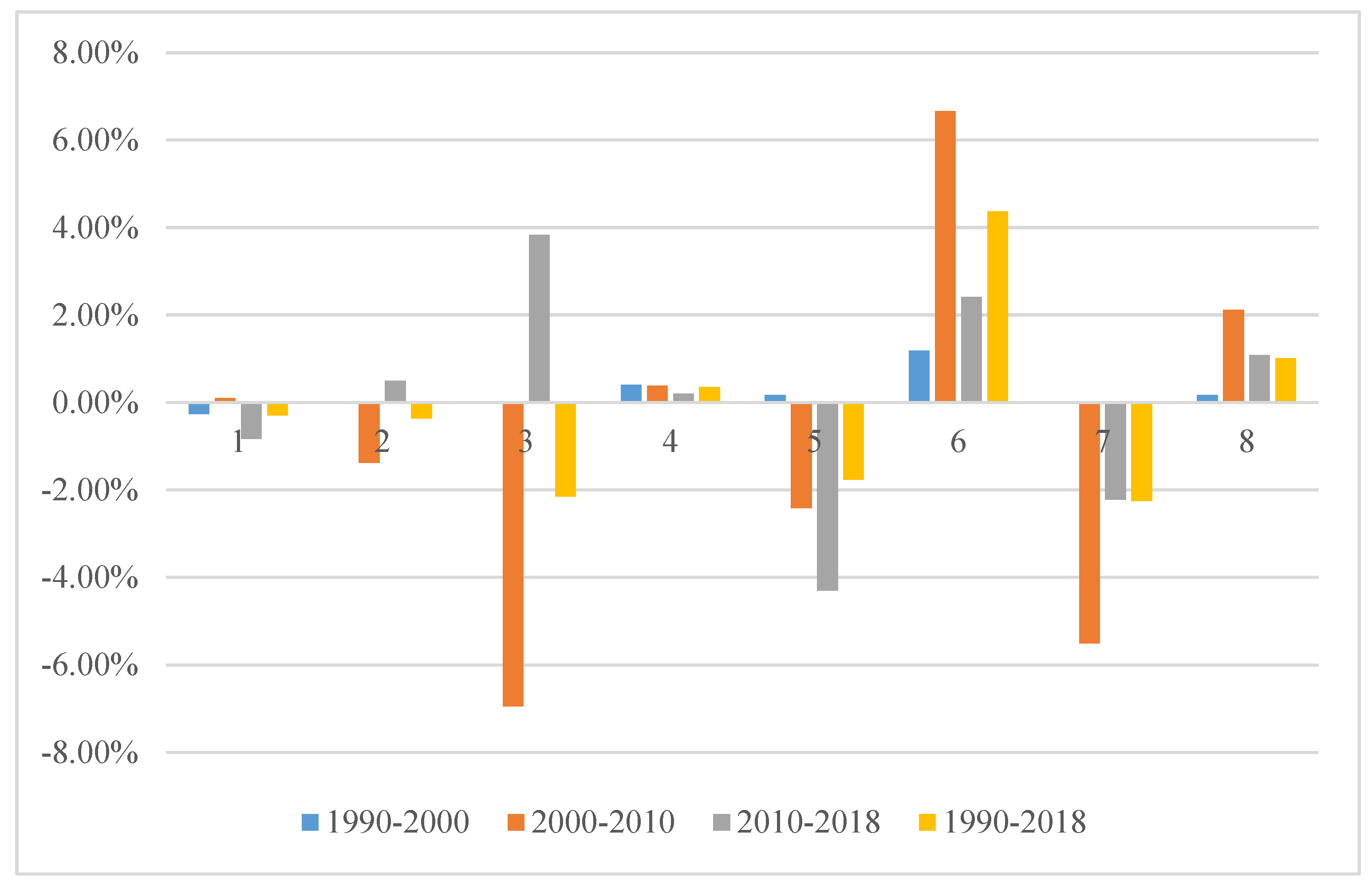
As can be seen in Figure 5, the rate of change of the percentage of built-up land, grassland, unused land, and salt-field and fish-farm areas in the study area was relatively fast, whereas the rate of change of the percentage of arable land, woodland, and wetlands and waters was relatively slow. The comprehensive dynamic attitude from 2000 to 2010 was the largest, whereas it was small from 1990 to 2000. Its code on the horizontal axis is 8 in Figure 5.

Built-up land always showed a fast growth rate in all periods. The percentage of the built-up land, woodland, grassland, and unused land changed dramatically from 2000 to 2010; the values of which were 6.66%, −1.38%, −6.95%, and −5.51%, respectively.

From 2000 to 2010, woodland and grassland showed rapid negative growth, exhibiting a dynamic attitude of −1.38% and −6.95%, respectively. From 2010 to 2018, the woodland and the grassland showed rapid positive growth, with dynamic attitudes of 0.50% and 3.83%, respectively. The direction of growth also changed.

3.2.2. Quantity Relation and Spatial Distribution of the Landscape Processes in Each Decade

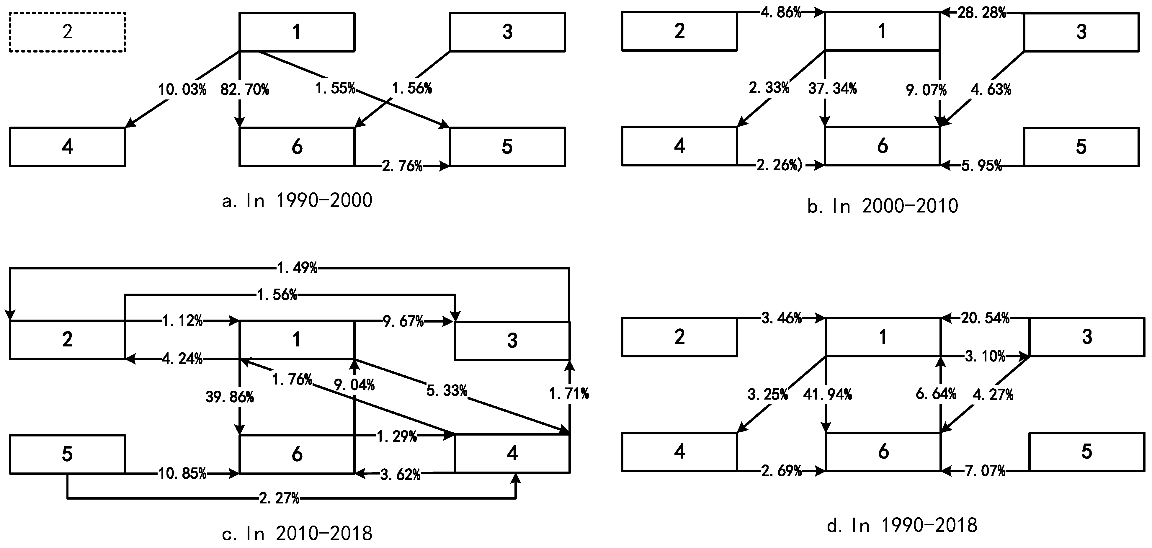
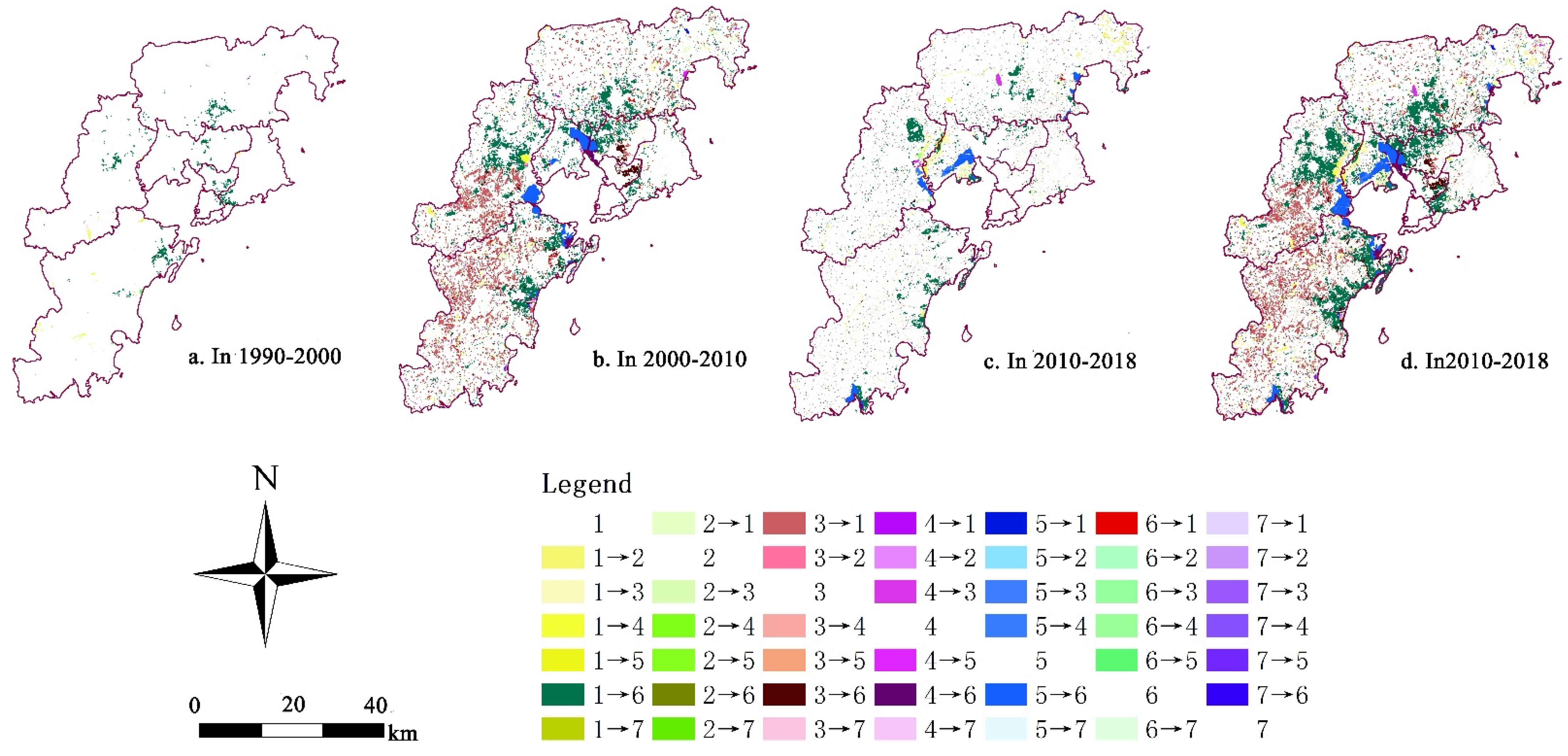
There were five major conversion relationships during 1990–2000, as shown in Figure 6a. Arable land and built-up land are the core landscape types of the landscape process. The conversion quantity from arable land to built-up land accounted for 82.70% of the transfer area. Its area was the largest, reaching 8954.64 ha, followed by the landscape process of arable land to wetlands and waters, at 1084.77 ha. Major conversion relationships did not include woodland types during this period.

Eight major conversion relationships accounted for 94.72% of the total conversion area between 2000 and 2010 (Figure 6b). The proportion of arable land to built-up land was still the highest, at 37.34%, followed by that of grassland to arable land, at 28.28%. Built-up land to arable land was another main relationship, accounting for 9.07%. In this period, the outflow of arable land and its inflow achieved equilibrium. Built-up land and grassland became sources of cultivated land. Woodland, built-up land, and grassland contributed 6545.07 ha, 12,216.87 ha, and 38,077.74 ha to the arable land. The total conversion area of the three was 56,839.68 ha. There was a significant net increase of 55,359.54 ha in the built-up land, whereas arable land contributed 50,283.54 ha. The above quantitative relations guarantee the tremendous growth of the built-up land without reducing the amount of cultivated land.

There were 14 major landscape processes between 2010 and 2018 (Figure 6c). There were mutual conversion relationships between landscape types, such as cultivated land and forest land, cultivated land and construction land, cultivated land and wetland and waters area, and forest land and grassland. Conversion of the arable land to the built-up land was still dominant, about 22,155.12 ha, accounting for 39.86%. Salt-field and fish-farm areas of approximately 6032.34 ha became one of the sources of built-up land, accounting for 10.85% of the transfer area.

During this period, the inflow of cultivated land was not enough to compensate for its outflow. The net decrease in the cultivated land from 2010 to 2018 was 24,239.07 ha. The grassland did not compensate for the arable land, and its amount did not exceed 1% of the total proportion. The other main supplementary channels have provided only 8607.06 ha of arable land. However, the area of the arable land transferred out to the built-up land, grassland, wetlands and waters, and woodland was 22,155.12 ha, 5375.25 ha, 2959.83 ha, and 2355.93 ha, respectively. The total area of arable land transferred out was 32,846.13 ha.

In the recent 30 years, from 1990 to 2018, there were nine major transformation relationships, accounting for 92.95%, and the 33 other transformation relationships accounted for 7.05% of the area (Figure 6d). Among them, the transformation of arable land to built-up land, grassland to arable land, built-up land to arable land, and salt-field and fish-farm to built-up land accounted for 41.94%, 20.54%, 6.64%, and 7.07% of the total area, respectively. Their areas were 75,587.11 ha, 37,016.19 ha, 11,936.7 ha, and 12,749.49 ha, respectively.

The landscape process of arable land to built-up land was distributed around the administrative center in Jimo, Jiaozhou, and the Chengyang District center. This process showed a diffuse distribution.

The spatial distribution of landscape processes is shown in Figure 7.

In 2000–2010, a large amount of grassland was transformed into cultivated land in the hilly region in the south of Jiaozhou District and the northwest of Huangdao District. In 2000–2018, salt-field and fish-farm and wetlands and waters near Jiaozhou Bay, Dagu River, Taoyuan River, and Yanghe River were transformed into construction land. The process of arable land outflowing to wetland, forest land, and grassland was scattered in various districts and counties.

Salt-field and fish-farm areas to built-up land presented the state as a concentrated distribution of blocks. The conversion from built-up land to arable land ringed around the rural residential areas. The shape of the woodland and grassland to arable land contour lines along the hills and valleys, like branches, in Huangdao and Chengyang.

3.2.3. Quantitative and Spatial Distribution Characteristics of All the Landscape Processes

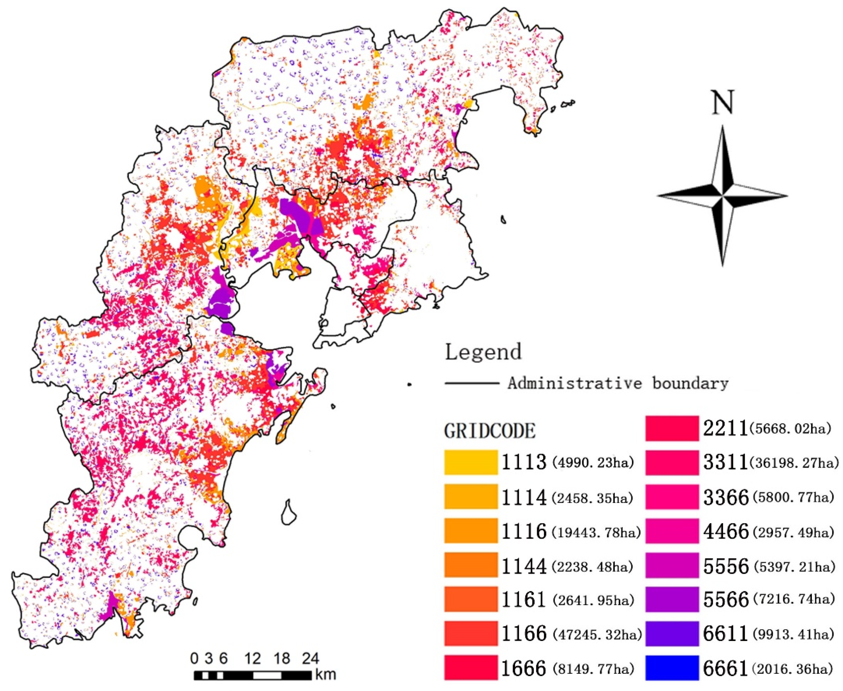
Through LCTA, we found that 15 transformation trajectories constitute the main landscape processes, which can be categorized into a landscape process of eight categories, as provided in

Table 5. Eight types of landscape processes based on the changes in the landscape trajectories.

Serial Number	Name	Main Trajectory Types
1	Outflow of built-up land	6611, 6661, 1161
2	Inflow of built-up land	5556, 5566, 1116, 1166, 1666, 3366, 4466
3	Outflow of ecological land	3311, 2211, 3366, 4466
4	Inflow of ecological land	1144, 1114, 1113
5	Outflow of arable land	1116, 1666, 1144, 1161, 1114, 1113, 1166
6	Inflow of arable land	1161, 3361, 2211, 6611, 6661
7	Outflow of salt-field and fish-farm	5556, 5566
8	Backflow of arable land	1161

. As long as the landscape processes take place in each decade, the entire landscape process will be classified into one of the eight categories. Therefore, for example, the “1161” type belongs to both the outflow and inflow of arable land, as well as the landscape process of backflow of arable land.

From the number of various landscape processes, we can see that the transfer trajectory had two directions. One was the inflow of the built-up land from arable land, grassland, salt-field and fish-farm, and the other part was the outflow of the arable land to the grassland and the built-up land. Among the 15 landscape types, the number of the “1116” trajectories was the highest, followed by “3311”, and “1116”, which corresponded to 47,245.32 ha, 36,198.27 ha, and 19,443.78 ha, respectively (Figure 8). The distribution characteristics of the landscape processes were similar to those in the previous section and thus will not be elaborated on here.

3.3. Spatial Distribution Heterogeneity of the Landscape Processes

3.3.1. Dynamic Pattern of the Landscape Processes Revealed by the Landscape Pattern Index

The NP index and AREA_MN index reflect the number of patches and the average area of patches in the landscape. It is worth noting that the ecological outflow landscape process has the largest number of patches. The average patch area is the smallest in the process of backflow of the arable land. The outflow and inflow of cultivated land and built-up land have many landscape patches. The NP index values are 2155, 2264, 2019, and 1959, respectively, indicating the existence of many patches in these landscape processes. The average patch area in the process of built-up land inflow is large. Its AREA_MN index is 50.3849. However, the AREA_MN index of the outflow of built-up land is 7.2452 (

Table 6. Landscape pattern index of the landscape process.

TYPE	NP	LSI	AREA_MN	SHAPE_MN	FRAC_MN	CONTIG_MN	AI
1	2019	48.9587	7.2452	1.0661	1.014	0.0758	19.3243
2	1959	46.1746	50.3849	1.1674	1.0234	0.1398	70.9811
3	726	42.1911	69.5813	1.4379	1.0487	0.2873	62.9769
4	542	23.0505	17.9262	1.093	1.0125	0.0604	54.129
5	2155	49.1554	40.4492	1.1528	1.0215	0.1231	67.0717
6	2264	56.6429	24.9435	1.1782	1.0238	0.1275	52.7002
7	28	7.708	449.2857	1.588	1.0566	0.5444	87.7287
8	600	24.8846	4.5067	1.0141	1.0031	0.0123	4.4615

).

The SHAPE_MN and FRAC_MN indices measure the shape regularity of the patches, whereas LSI measures the degree of overall regularity at the landscape level. The SHAPE_MN index of outflow of the ecological landscape is 1.4379, indicating that the patches are irregular in shape. Similarly, its LSI is 42.1911, indicating that its patches and overall landscape process are irregular. The SHAPE_MN index of the processes of built-up land inflow, ecological land inflow, and arable land backflow is 1.0661, 1.093, and 1.0141, respectively, indicating that the patches of the above three landscape processes are relatively regular. Similarly, ecological land inflow and arable land backflow are more regular on the landscape scale because their LSI index values are small, namely, 23.0505 and 24.8846, respectively. However, the LSI index of the built-up land inflow is large, indicating that its overall shape in the landscape is irregular.

The AI index and CONTIG_MN index of the ecological land outflow, arable land outflow, arable land inflow were all high, indicating that the degree of patch connectivity and the degree of aggregation of the landscape processes are high. The CONTIG_MN landscape index of the process of ecological inflow landscape is 0.0604, but its AI index is 54.129. Although the CONTIG_MN is not high, its high AI index indicates that the overall degree of aggregation of this kind of landscape process is high, but the landscape connectivity within each patch is poor. The CONTIG_MN index of the landscape processes of built-up land outflow and arable land backflow is 0.0758 and 0.0123, respectively, and the AI index is 19.3243 and 4.4615, respectively (Table 6). The degree of connectivity in these patch types is not good, and the overall distribution and degree of aggregation of the landscape processes are not high.

The outflow of salt-field and fish-farm areas is a more specific landscape process. The outflow of salt-field and fish-farm areas has the minimum NP and LSI index values and maximum AREA_MN, SHAPE_MN index values. The statistics are 28, 7.708, 449.2857, and 1.588, respectively, indicating that there are fewer patches but that they are large patches. The overall landscape shape is relatively regular, but the landscape patches are not. In terms of the degree of aggregation and connectivity, the CONTIG_MN index and the AI index are 0.5444 and 87.7287, respectively (Table 6). This indicates that the patches have good connectivity, and the aggregation in the overall landscape process is high.

3.3.2. Spatial Heterogeneity of the Various Landscape Processes Analyzed Using Spatial Autocorrelation

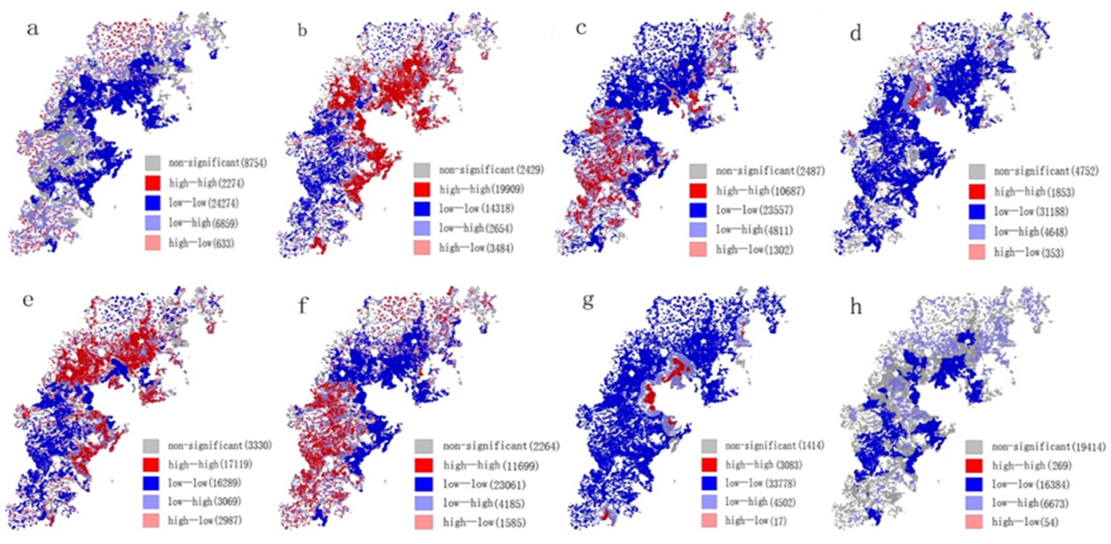
Using the GeoDa1.12 software, the global Moran index scatter plots were obtained. All the results passed the hypothetical test and could be used for further analysis. The Moran index values of the eight landscape processes are 0.149, 0.488, 0.465, 0.25, 0.454, 0.503, 0.550, and 0.016, respectively. Among five landscape processes, the Moran index is relatively high, and there are more “high-high” and “low-low” aggregations. This shows that the landscape processes are more concentrated in space. Further, the local Moran analysis is meaningful for them. However, the other landscape processes are relatively scattered in space.

The information of the spatial relevance between the adjacent area could not be incorporated in the global Moran index. Therefore, in this study, further analysis of the local indicator of spatial association obtained from the LISA cluster diagram (Figure 9) was performed. The eight pictures correspond to the eight landscape processes in Table 5.

As can be seen from Figure 9a, the “high-high” aggregation of the outflow of built-up land is concentrated in the suburbs and rural areas of Jimo, Jiaozhou, and Huangdao districts, in the suburban and rural areas far from the coast. Its distributions are intertwined with the “low-high” aggregation type. About 2274 grid cells exhibit “high-high” aggregation, which is relatively dispersed, and 6859 grid cells exhibit the “low-high” aggregation state and are relatively concentrated. As is seen from Figure 9b, the “high-high” aggregation of inflow of built-up land is concentrated around Jiaozhou Bay, the administrative center, the Huangdao economic development zone, and the Hongdao high-tech zone. Further, 19,909 grid units exhibit a “high-high” aggregation state.

The “high-high” aggregation of ecological land outflow is concentrated in the hilly area west of Jiaozhou Bay with a relatively high elevation and exhibits a fragmented distribution (Figure 9c). Further, 10,687 grid units exhibit a “high-high” aggregation. At the same time, the “high-high” aggregation in the landscape process of inflow of the ecological land is mainly distributed along the periphery of the Taoyuan and Dagu rivers (Figure 9d).

In the outflow of arable land (Figure 9e), the “high-high” aggregation is distributed around the periphery of Jiaozhou and Jimo administrative center, with 17,119 grid units. Large areas of arable land around the city have been occupied. It is clear from Figure 9f that the “high-high” aggregation of arable land outflow is distributed in the hilly areas west of Jiaozhou Bay and the rural areas in Huangdao and Jimo, interweaving with the “low-high” aggregated grid units. Reclamation of rural residential areas and development of grassland might be able to explain this spatial distribution.

The outflow of salt-field and fish-farm is distributed along the coast of Jiaozhou Bay, in the Hongdao high-tech zone and Dongjiakon Port (Figure 9g). Local indicators of spatial association are not significant in the backflow of arable land in the study area (Figure 9h).

3.4. Factors Driving the Spatial Heterogeneity of the Various Landscape Processes Obtained Using the OPGD Model

3.4.1. Important Influencing Factors Revealed by Q-Statistic

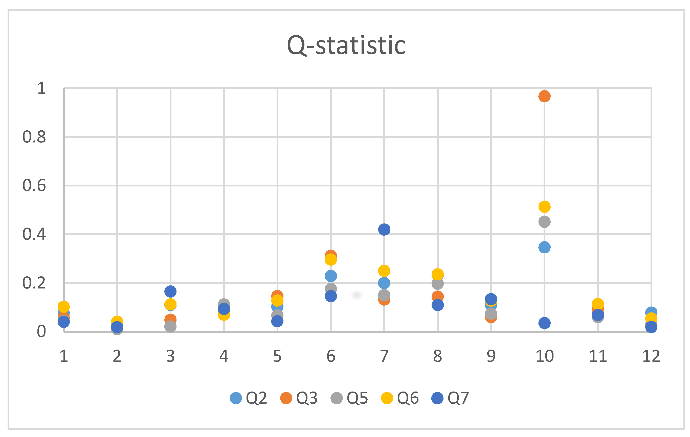
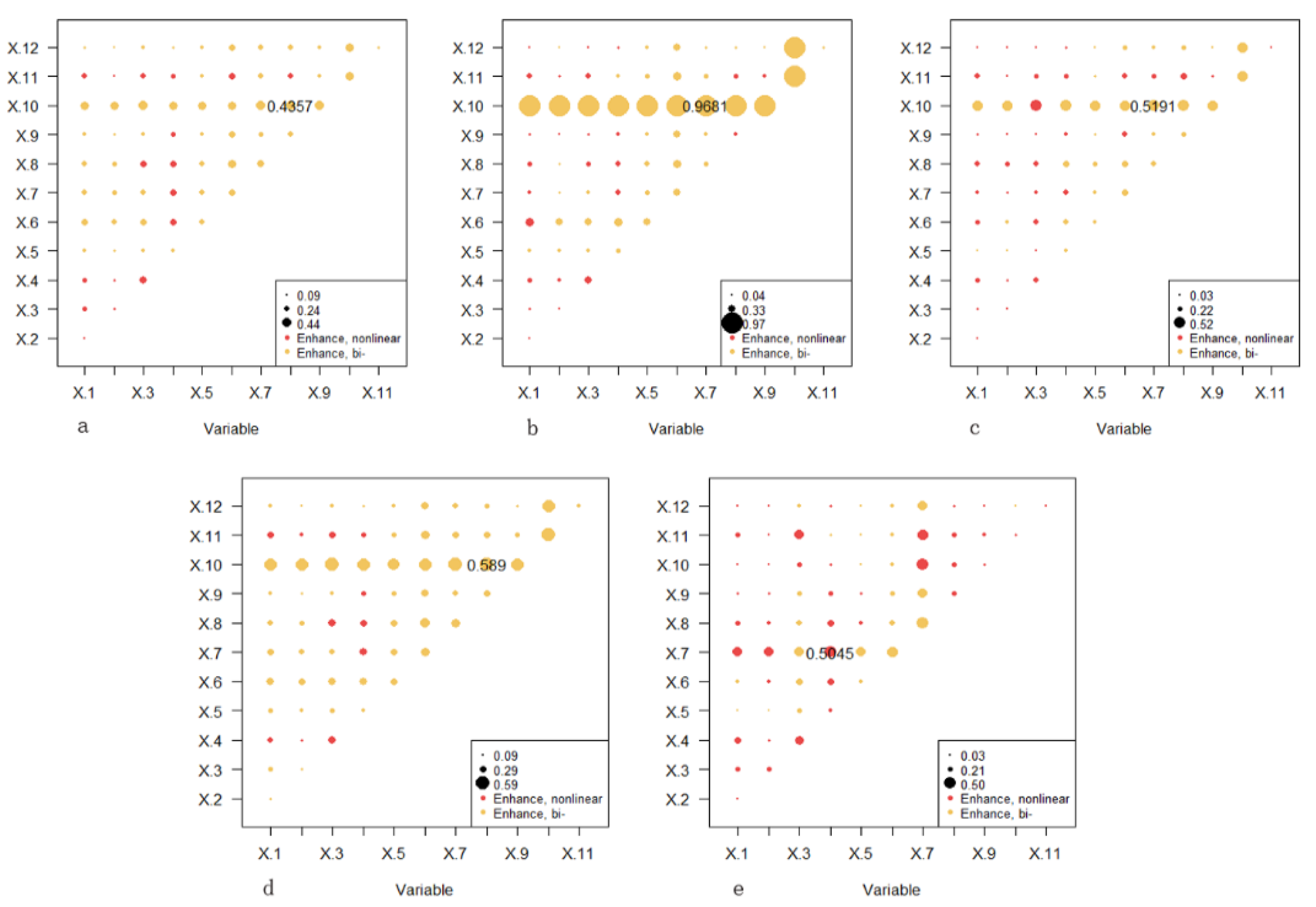
The results of the factor detector and interaction detector are shown in Figure 10 and Figure 11 from, which the following is observed: X10 has the greatest influence on the five landscape processes except for the outflow of salt-field and breeding area. X6, X7, and X8 also exhibit a huge impact on the different landscape processes. The abovementioned driving factors are all over 0.1. However, X2 and X12 have no more than 0.1 influence factors on the five landscape processes. X1 and X11 have a smaller influence factor, close to 0.1. Factors were selected as in Table 2.

From the interactive detector results shown in Figure 11, it can be observed that the interaction between the Q-statistic is shown as bivariable-enhance or nonlinear-enhance; there is no independent or weakened state. The interaction between the different factors has different degrees of enhancement. It is also confirmed that the landscape process is a kind of complex factor interaction process.

3.4.2. Results of the Geographical Detector for the Major Landscape Processes

(1) Inflow of built-up land

The order of the significant Q-statistic (value > 0.1) corresponding to this landscape process is as follows: X10 > X8 > X6 > X7 > X9 > X3 (Figure 10). The variables with a strong influence (Q-statistic greater than 0.2) are X10, X8, and X6, respectively. In this landscape process, the interactions between X1, X2, X3, X4, and X7, X8, X9 are nonlinear-enhancement. In addition, the interactions between X5, X7, X10, X11, and other factors are also non-linear enhancement (Figure 11). This indicates that the interaction statistics are larger than the sum of the two Q-statistics. The variable of X10 and other variables jointly promote the landscape process greatly. The largest interaction variables are X8 and X10, and the interaction statistic is 0.4527. This value is greater than the maximum Q-statistic of X8 and X10.

By comparing the values of the risk mean, the following was observed. For the inflow of built-up land, the risk mean attribute values in different ecological landscape types are different. For X10, the risk mean in nonecological landscape types is 0.75. For lakes, tidal flats, and reservoirs, the landscape process attribute value is approximately equal to 0.9. For woodland, the attribute value is 0. This indicates that large amounts of inflow of built-up land are distributed in wetlands and waters, whereas the woodland is not converted to built-up land. For X8, the risk mean value is large in the two intervals (0, 2180), (4400, 61,200). These values are more than 0.6 or even close to 0.9. In X3, X6, X7, the higher the interval value, the lower the risk mean value. This shows that the farther away from the coast, the higher the elevation and vegetation coverage, and the inflow of the built-up land is less.

(2) Outflow of ecological land

The order of the significant Q-statistic (value > 0.1) for this landscape process is as follows: X10 > X6 > X5 > X8 > X7 > X4 (Figure 10). Similar to the case of the inflow of built-up land, X10, X6, X8, and X7 are the major factors. However, X4 and X5 are important influencing factors; an observation which is contrary to that for the inflow of built-up land. The factors with strong explanatory power (Q-statistic greater than 0.2) are X10 and X6. In this landscape process, the interactions between X1, X2, X3 and X2, X3, X4, X6, X7, X8, X9, X11, X12 are almost nonlinear-enhance (Figure 11). The interactions between X4 and X7, X8, X9 as well as the interactions between X8 and X9, X10 are also nonlinear-enhance. The interactions corresponding to X10 are significant in the interaction statistic matrix. The type of ecological landscape greatly promotes the landscape process. The four distance variables enhance others on the formation of ecological land outflow.

By comparing the risk mean, the following was observed. For X10, the mean risk of the landscape process in the nonecological landscape types is 0. Except for 41 and 46 in the CNLUCC, the mean risk values of the other types are greater than 0.95. The outflow of ecological land is generally distributed in the ecological landscape types, however, not in Graff and Bottomland. In X6, X5, X7, the higher the interval value, the higher is the mean risk value. The minimum and maximum values of the interval are 0.17 and 0.53 for X7, 0.09 and 0.82 for X6, and 0.14 and 0.78 for X5, respectively. This shows that the higher the elevation, the higher is the vegetation coverage, and the greater is the slope, which leads to the outflow of the ecological landscape. In X4, the higher value of the landscape process is concentrated in the range of (3160, 13,400), and its value is about 0.5, indicating considerable outflow of the ecological landscape in the range of 3160 m to 13,400 m from the central town, i.e., in the suburban region. In X9, it is clear that the population increase will promote the outflow of the ecological landscape, but the process occurs less in regions with excessively high population growth.

(3) Outflow of arable land

The order of the significant Q-statistic (value > 0.1) is as follows: X10 > X8 > X6 > X7 > X4. The variables with strong influence (value > 0.2) are X10, X8, and X6, respectively. The main factors influencing the arable land outflow and built-up land inflow into the landscape are similar, but X4 is an important influencing factor corresponding to farmland outflow. In this landscape process, the interactions between X1, X2, X3, X4, and X6, X7, X8, X9, X11, X12 are nonlinear-enhance. The interaction factors between X3 and X10 are also nonlinear enhance. The interaction value is 0.5440 between X7 and X10. The above situation shows that the ecological landscape type, the distance from the coast, and the normalized difference vegetation index (NDVI), implemented from October 1998, influenced the landscape process.

By comparing the risk mean, the following was observed. For X10, the risk mean in the nonecological landscape type is 0.73, whereas for the other types, it is 0. This indicates that the outflow of cultivated land is not within the spatial scope of any ecological landscape type. In X8, in an interval of (4400, 612,000), the risk mean value is more than 0.6, which implies that the arable land outflow is high in this range. In X6, cultivated land outflow focused on the elevation below 100. In X7, in an interval of (0.41, 0.656], the risk mean value is more than 0.7. The distribution of arable land flow in that vegetation coverage is not very high. In X4, the higher value is concentrated in the range of (20,800, 62,000], and its value is more than 0.5, indicating that the outflow of arable land in the range from 20,800 m to 62,000 m is more, i.e., far away from the center of the town.

(4) Inflow of arable land

The order of the significant Q-statistic (value > 0.1) for the landscape process of outflow of arable land is as follows: X10 > X6 > X7 > X8 > X5 > X9 > X11> X3 > X1. Similar to the results for the inflow of built-up land and outflow of ecological land, X10, X6, X8, X7 are the major factors. In contrast to the abovementioned landscape processes, the inflow of arable land has a large number of factors with strong influence. Except for X2, X4, and X12, the explanatory power of all factors exceeds 0.1. The values of X1 and X11 variables are greater than 0.1, contrary to the observations corresponding to the above processes. In this landscape process, the interactions between X1, X2, X3, and X4 are nonlinear-enhance. The interaction variables between X4 and X7, X8, X9, X11 are also nonlinear-enhance. The same is true for the interaction factors between X11 and X1, X3, X4, and between X8 and X9, X10. The maximum interaction variable value is 0.5997 between X8 and X10.

By comparing the risk mean values, the following was observed. For X10, the impact on the ecological landscape type exhibits a significant difference. The inflow of the arable landscape process is distributed between the woodland and grassland. In other words, the grassland and woodland have been transformed into arable land. In X8, in an interval of (2180, 4400), the risk mean is more than 0.48, which implies that the arable land inflow is greater in this area. In X3, X5, X6, and X7, the higher the elevation, the higher the vegetation coverage, the greater is the slope, and the farther is the distance from the coast, which leads to the larger inflow of arable land. In X9, in the interval (573, 12,900], the population growth is huge, but the arable land inflow is less. The risk mean of X1 shows that landscapes far away from the center of the development zone are easily transformed into arable land. The risk mean of X11 shows that the administrative regions that have large fixed investment growth have more arable land growth, such as the Huangdao, Jimo, and Jiaozhou districts.

(5) Outflow of salt-field and fish farm

The order of significant Q-statistic (value > 0.1) is as follows: X7 > X3 > X6 > X9 > X8. The factor with a strong explanatory power (Q-statistic greater than 0.2) is X7. This situation reflects that this landscape process is influenced by the population difference, GDP in 1995, elevation, and distance from the shore. In this landscape process, there are many cases of nonlinear-enhance, indicating that the interactions of each variable are stronger in this landscape process as compared to that for the other landscape processes. The interactions between X7 and X4 are the largest, and the interaction statistic is 0.55, which is greater than the sum of X4 and X7.

From the risk mean values of X7, X3, X6, X9, and X8, it is observed that the outflow of aquaculture landscape in the low vegetation coverage areas is more. The areas having lower elevation and, which are closer to the coast have more outflow of salt-field and fish farm, whereas the areas having higher elevation do not have the outflow of salt-field and fish farm.

4. Discussion

4.1. The Spatiotemporal Difference of Landscape Processes Affected by The Change of Land Use Pattern and Economic Development

The study area is a typical bay area with high development activity and is located in Qingdao, an important coastal port city. The development of the national economy and the utilization of territorial resources in the past 30 years have greatly transformed the landscapes in the Jiaozhou Bay coastal zone. The proportion of stable and unchanged landscape was 0.716, and the changed landscape was 180,228.42 ha, accounting for 28.4%. Such a large number of landscape changes are related to the rapid development of the Jiaozhou Bay area in Qingdao. The statistical yearbook shows that the GDP of the eight administrative districts in Jiaozhou Bay (adjusted by region) increased from 13.2 billion yuan in 1990 to 104 billion yuan, and the resident population increased from 4.7 million in 1990 to 7.2 million in 2018. With the rapid economic as well as population growth, there was an urgent need for the built-up land to meet the demand. Thus, much of the landscape change was inevitable.

In terms of the speed of the change, the grassland, salt-field and fish farm, and built-up land has changed dramatically. The single dynamic degree of the three types is higher than the comprehensive dynamic attitude. Although the single dynamic degree of arable land is not high, the proportion of arable land has changed significantly. From 1990 to 2018, on the one hand, 75,582 ha of arable land was converted to built-up land. On the other hand, 37,016.19 ha of grassland and 11,963.7 ha of built-up land were used for supplementing the arable land. The right to develop the land has always been in the hands of the government. The obligation of protecting arable land also falls on the government. The Land Administration Law of the People’s Republic of China (revision in 1998) has implemented a “requisition-compensation balance” policy of arable land [35]. Through the land-use regulation system, agricultural land is protected from excessive real estate and industrial development. Extensive rural land consolidation was carried out in 2007 [36]. The implementation of the above policy has been confirmed in the present study. The amount of cultivated land in the Jiaozhou Bay region showed a balanced state from 2000 to 2010, maintained at 387,605.25 ha. Built-up land outflows are mostly in rural areas. In this way, the balance between cultivated land and the growth of built-up land was ensured at the expense of grassland, built-up land, wetland and waters, salt-field breeding, and other landscape types.

4.2. Internal Relations among the Various Spatial Distribution of Landscape Processes

From the spatial heterogeneity analysis of the different landscape processes, we found five landscape processes exhibiting a strong spatial autocorrelation, namely, the inflow of built-up land, the outflow of ecological land, the outflow of arable land, the inflow of arable land, and the outflow of salt-field and fish farm areas. The strong spatial autocorrelation indicates that the aggregation of the landscape processes is very high. It also shows that other landscape processes are highly dispersed in space.

From the distribution map of the landscape processes and the LISA cluster diagram (Figure 9), it can be seen that the inflow of the built-up land is mainly distributed in Jiaozhou, the Jimo administrative center, and the coast of Jiaozhou Bay, exhibiting a “high-high” distribution. Over the years, Qingdao has been adhering to the principle of “development around the bay”. It can also be seen that there is a large amount of built-up land inflow in the state-planned economic development zones. Arable land outflow and built-up land inflow exhibit the distribution characteristics of convergence. In China, there is a huge inflow of built-up land around major towns and national development zones. Another typical feature is that the expansion of urban construction land occupies the surrounding cultivated land [37]. The higher AREA_MN, CONTIG_MN, and AI index values indicate that the development of cultivated land and expansion of urban construction land has the characteristics of concentration and contiguity (Table 6).

The landscape processes of ecological outflow and cultivated land inflow are distributed in the hilly area west of Jiaozhou Bay. Combined with the huge amounts of outflow of ecological land in Jiaozhou Bay, it is not difficult to find that it is the source of the balance between the cultivated land occupation and compensation. The LISA cluster diagram indicates that the inflow of arable land and the outflow of ecological land has high similarity. Many grasslands have been reclaimed into arable land in the western hilly area to supplement the lost arable land. It leads to the mean center of the grassland landscape moving eastward (Figure 4). The NP, LSI, and SHAPE_MN indices show that the process of arable land inflow and ecological land outflow is relatively dispersed, and the patches are out of regular shape. The arable land reclamation is greatly affected by the topography of the hilly areas. Salt-field and fish farm areas in northern Jiaozhou Bay were nationalized via land expropriation and were transformed into construction land.

4.3. Natural Changes, Economic and Social Development and Planning Affecting Landscape Processes

It has been found that the landscape process that has a strong spatial autocorrelation often has a higher Q-statistic in the factor detector and vice versa. Therefore, five landscape processes were selected in this study for analysis, and the factors driving them were investigated. The results thus obtained show that the types of ecological landscape, the distance from cities and towns, slope, elevation, NDVI implemented from October 1998, and the GDP in 1995 are the main factors that have affected the five landscape processes. Different ecological types have a great influence on landscape processes. It can be seen that the main source of supplementary arable land is grassland. In contrast, the direct sources of construction land are not the ecological landscape, such as the forest land and grassland, but the landscape types, such as cultivated land, salt-field and fish farms, and wetlands and waters. The outflow of the ecological landscape is distributed between all kinds of landscape types. With the development during the past 30 years, the ecological landscape has been damaged, and the outflow of ecological land is widespread.

The higher elevation, slope, and vegetation coverage have led to less built-up land inflow. However, arable land inflow and ecological land outflow present the opposite situation. The outflow of ecological land was not easily affected by the distance from the coast, which is similar to the results observed for the outflow of arable land. Ecological land outflow is distributed at the outskirts of central towns, whereas arable land outflow is mostly distributed in the outer suburbs.

5. Conclusions

By using remote sensing images, we have analyzed the Spatiotemporal heterogeneity of the landscape process.

The influence of landscape processes on landscape types in the Jiaozhou Bay area over the last 30 years has been significant, especially between 2000–2010. The inflow of built-up land has brought about a dramatic expansion in the amount of build-up land, by 92,311.11 ha, with most of this expansion occurring in the suburbs of the city. The expansion of built-up land comes at the expense of prime arable land around the city, accompanied by arable land outflow. However, the change in the amount of arable land is not significant due to the ecological land outflow and built-up land outflow in rural areas. China’s “requisition-compensation balance” policy and rural land reclamation play a large role.

The heterogeneity in the spatial distribution of landscape processes is more pronounced. The landscape pattern index shows a large number of patches and connectivity in arable land outflow and built-up land inflow. The outflow of salt-field and fish-farm areas has the highest degree of aggregation and the largest patch size. The shape of ecological land outflow is most irregularly. The LISA cluster diagram revealed that, despite the spatial heterogeneity of landscape processes, several landscape processes had relatively similar characteristics, for example, ecological land outflow and arable land inflow, built-up land inflow, and arable land outflow.

Landscape processes are affected by the elevation, slope, distance from the coast, and, especially, ecological types. The results of the OPDG model show that a gentler slope and lower elevation, and proximity to cities and town land will produce more arable land outflow and built-up land inflow. However, arable land inflow and ecological land outflow present the opposite situation. The impact of landscape processes is significant when they involve ecological land types.

This study can provide lessons for natural resource managers in the rapidly developing coastal zone area and contribute to the study of landscape processes. Land-use planning and climate change may have an impact on landscape processes. In a future study, it is necessary to explore their impact on the landscape process by a similar method.

References

1. Déjeant-Pons, M. The European landscape convention. Landsc. Res. 2006, 31, 363–384. [Google Scholar] [CrossRef]
2. Wu, J.G. Landscape Ecology: Pattern, Process, Scale, and Hierarchy, 2nd ed.; Higher Education Press: Beijing, China, 2017; pp. 17–40. [Google Scholar]
3. Fu, B.J.; Chen, L.D.; Ma, K.M.; Wang, Y.L. Principles and Applications of Landscape Ecology, 2nd ed.; Science Press: Beijing, China, 2011; pp. 44–51. [Google Scholar]
4. Chen, L.D.; Liu, Y.; Lv, Y.H.; Feng, X.; Fu, B. Landscape pattern analysis in landscape ecology: Current, challenges and future. Acta Ecol. Sin. 2008, 28, 5521–5531. [Google Scholar]
5. Bičıík, I.; Jeleček, L.; Štěpánek, V. Land-use changes and their social driving forces in Czechia in the 19th and 20th centuries. Land Use Policy 2001, 18, 65–73. [Google Scholar] [CrossRef]
6. Käyhkö, N.; Skånes, H. Retrospective land cover/land use change trajectories as drivers behind the local distribution and abundance patterns of oaks in south-western Finland. Landsc. Urban Plan. 2008, 88, 12–22. [Google Scholar] [CrossRef]
7. Rong, F.F.; Tashpolat, T.; Tian, Y.; Zhang, F. Spatio-temporal Trajectory Analysis of Land Use/Cover Change in Oasis of Yutian. Res. Soil Water Conserv. 2010, 17, 259–263. [Google Scholar]
8. Southworth, J.; Nagendra, H.; Tucker, C. Fragmentation of a Landscape: Incorporating landscape metrics into satellite analyses of land-cover change. Landsc. Res. 2002, 27, 253–269. [Google Scholar] [CrossRef]
9. Wang, D.C.; Guo, J.H.; Chen, L.D.; Zhang, L.H.; Song, Y.Q.; Yue, Y.J. Spatio-temporal pattern analysis of land use/cover change trajectories in Xihe watershed. Int. J. Appl. Earth Obs. Geoinf. 2012, 14, 12–21. [Google Scholar] [CrossRef]
10. Zhou, Q.; Li, B.; Kurban, A. Spatial pattern analysis of land cover change trajectories in Tarim Basin, northwest China. Int. J. Remote Sens. 2008, 29, 5495–5509. [Google Scholar] [CrossRef]
11. Crews-Meyer, K.A. Agricultural landscape change and stability in northeast Thailand: Historical patch-level analysis. Agric. Ecosyst. Environ. 2004, 101, 155–169. [Google Scholar] [CrossRef]
12. Liu, J.; Wang, D.C.; Sun, R.H. Study on spatial relevance of ecological-land loss based on change trajectory analysis method. Geogr. Res. 2020, 39, 103–114. [Google Scholar]
13. Li, X.; Kuang, W.H. Spatio-Temporal Trajectories of Urban Land Use Change during 1980–2015 and Future Scenario Simulation in Beijing-Tianjin-Hebei Urban Agglomeration. Econ. Geogr. 2019, 39, 187–194. [Google Scholar]
14. Wang, D.C.; Gong, J.H.; Chen, L.D.; Zhang, L.H.; Song, Y.Q.; Yue, Y.J. Comparative analysis of land use/cover change trajectories and their driving forces in two small watersheds in the western Loess Plateau of China. Int. J. Appl. Earth Obs. Geoinf. 2013, 21, 241–252. [Google Scholar] [CrossRef]
15. Arnold, C.; Wilson, E.; Hurd, J.; Civco, D. 30 Years of Land Cover Change in Connecticut, USA: A Case Study of Long-Term Research, Dissemination of Results, and Their Use in Land Use Planning and Natural Resource Conservation. Land 2020, 9, 255. [Google Scholar] [CrossRef]
16. Corbelle-Rico, E.; Butsic, V.; Enríquez-García, M.J.; Radeloff, V.C. Technology or policy? Drivers of land cover change in northwestern Spain before and after the accession to European Economic Community. Land Use Policy 2015, 45, 18–25. [Google Scholar] [CrossRef]
17. Long, H.L.; Tang, G.P.; Li, X.B.; Heilig, G.K. Socio-economic driving forces of land-use change in Kunshan, the Yangtze River Delta economic area of China. J. Environ. Manag. 2007, 83, 351–364. [Google Scholar] [CrossRef] [PubMed]
18. Schweizer, P.E.; Matlack, G.R. Factors driving land use change and forest distribution on the coastal plain of Mississippi, USA. Landsc. Urban Plan. 2014, 121, 55–64. [Google Scholar] [CrossRef]
19. Wang, J.; Chen, Y.Q.; Shao, X.M.; Zhang, Y.Y.; Cao, Y.G. Land-use changes and policy dimension driving forces in China: Present, trend and future. Land Use Policy 2012, 29, 737–749. [Google Scholar] [CrossRef]
20. Dutilleul, P. Spatio-Temporal Heterogeneity: Concepts and Analyses; Cambridge University Press: London, UK, 2011. [Google Scholar]
21. Anselin, L. Local Indicators of Spatial Association-LISA. Geogr. Anal. 1995, 27, 93–115. [Google Scholar] [CrossRef]
22. Getis, A.; Ord, J. The Analysis of Spatial Association by Use of Distance Statistics. Geogr. Anal. 1992, 24, 189–206. [Google Scholar] [CrossRef]
23. Ord, J.K.; Getis, A. Local Spatial Autocorrelation Statistics: Distributional Issues and an Application. Geogr. Anal. 1995, 27, 286–306. [Google Scholar] [CrossRef]
24. Wang, J.F.; Li, X.H.; Christakos, G.; Liao, Y.L.; Zhang, T.; Gu, X.; Zheng, X.Y. Geographical detectors-based health risk assessment and its application in the neural tube defects study of the Heshun region, China. Int. J. Geogr. Inf. Sci. 2010, 24, 107–127. [Google Scholar] [CrossRef]
25. Wang, J.F.; Zhang, T.L.; Fu, B.J. A measure of spatial stratified heterogeneity. Ecol. Indic. 2016, 67, 250–256. [Google Scholar] [CrossRef]
26. Song, Y.Z.; Wang, J.F.; Ge, Y.; Xu, C.D. An optimal parameters-based geographical detector model enhances geographic characteristics of explanatory variables for spatial heterogeneity analysis: Cases with different types of spatial data. GISci. Remote Sens. 2020, 57, 593–610. [Google Scholar] [CrossRef]
27. Wang, J.F.; Xu, C.D. Geodetector: Principle and prospective. Acta Geogr. Sin. 2017, 72, 116–134. [Google Scholar]
28. Song, Y.Z. Optimal Parameters-Based Geographical Detectors (OPGD) Model for Spatial Heterogeneity Analysis and Factor Exploration, 12 June 2021. Available online: https://cran.r-project.org/web/packages/GD/index.html (accessed on 31 May 2021).
29. Xu, X.L.; Liu, J.Y.; Zhang, S.W.; Li, R.D.; Yan, C.Z.; Wu, S.X. A Multi-Period Remote Sensing Monitoring Dataset of Land Use and Cover in China (CNLUCC), Data Registration and Publication System of Resource and Environment Science and Data Center, Chinese Academy of Sciences. 2018. Available online: https://www.resdc.cn/DOI/doi.aspx?DOIid=54 (accessed on 31 May 2021).
30. Liu, J.Y.; Kuang, W.H.; Zhang, Z.X.; Xu, X.L.; Qin, Y.W.; Ning, J.; Zhou, W.C.; Zhang, S.W.; Li, R.D.; Yan, C.Z. Spatiotemporal characteristics, patterns, and causes of land-use changes in China since the late 1980s. J. Geogr. Sci. 2014, 24, 195–210. [Google Scholar] [CrossRef]
31. Zhu, H.Y.; Li, X.B. Discussion on the Index Method of Regional Land Use Change. Acta Geogr. Sin. 2003, 58, 643–650. [Google Scholar]
32. McGarigal, K.; Cushman, S.A.; Ene, E. FRAGSTATS v4: Spatial Pattern Analysis Program for Categorical and Continuous Maps. Computer Software Program Produced by the Authors at the University of Massachusetts, Amherst. Available online: http://www.umass.edu/landeco/research/fragstats/fragstats.html (accessed on 31 May 2021).
33. Huang, Y.; Wang, F.Y.; Cai, T.J.; Wang, D.C.; WANG, Q.Q.; Chen, W.G. Landscape Pattern Dynamic Analysis Based on Change Trajectory Method in Bohai Rim Area. Res. Soil Water Conserv. 2015, 29, 314–319. [Google Scholar]
34. Cliff, A.D.; Ord, J.K. Spatial Autocorrelation; London Point Ltd.: London, UK, 1973. [Google Scholar]
35. Liu, L.; Liu, Z.J.; Gong, J.Z.; Wang, L.; Hu, Y.M. Quantifying the amount, heterogeneity, and pattern of farmland: Implications for China’s requisition-compensation balance of farmland policy. Land Use Policy 2019, 81, 256–266. [Google Scholar] [CrossRef]
36. Chen, W.; Ye, X.; Li, J.; Fan, X.; Liu, Q.; Dong, W. Analyzing requisition–compensation balance of farmland policy in China through telecoupling: A case study in the middle reaches of Yangtze River Urban Agglomerations. Land Use Policy 2019, 83, 134–146. [Google Scholar] [CrossRef]
37. Song, W.; Pijanowski, B.C.; Tayyebi, A. Urban expansion and its consumption of high-quality farmland in Beijing, China. Ecol. Indic. 2015, 54, 60–70. [Google Scholar] [CrossRef]
Figure 1. Landscape processes at different monitoring points in time.
Land 11 00007 g001
Figure 2. Developing and highly developed region in the study area.
Land 11 00007 g002
Figure 3. Spatial distribution of various types of landscape. (a) 1990, (b) 2000, (c) 2010, (d) 2018.
Land 11 00007 g003
Figure 4. Map showing the migration of the mean center of the different landscape types.
Land 11 00007 g004
Figure 5. Single and comprehensive dynamic attitude of the landscape processes in each decade.
Land 11 00007 g005
Figure 6. Proportion of landscape processes to overall processes in each decade. (a) During the period 1990–2000; (b) During the period 2000–2010; (c) During the period 2010–2018; (d) During the period 1990–2018.
Land 11 00007 g006
Figure 7. Spatial distribution of the various landscape processes in each decade. (a) During the period 1990–2000; (b) During the period 2000–2010; (c) During the period 2010–2018; (d) During the period 2010–2018.
Land 11 00007 g007
Figure 8. Map showing the changes in the trajectories of the landscape processes.
Land 11 00007 g008
Figure 9. LISA cluster diagram of the different landscape processes. (a) Outflow of built-up land; (b) Inflow of built-up land; (c) Outflow of ecological land; (d) Inflow of ecological land; (e) Outflow of arable land; (f) Inflow of arable land; (g) Outflow of salt-field and fish-farm; (h) Backflow of arable land.
Land 11 00007 g009
Figure 10. Q-statistic for each landscape process. (Q2, Q3, Q5, Q6, Q7 corresponding to the serial number of landscape processes 2,3,4,6,7 in Table 5; Abscissa 1-12 corresponding to the data number in Table 2).
Land 11 00007 g010
Figure 11. Interactions between the two explanatory variables and their interactive statistic. (a) Interaction Q-statistic of inflow of built-up land; (b) interaction Q-statistic of outflow of ecological land; (c) interaction Q-statistic of outflow of arable land; (d) interaction Q-statistic of inflow of arable land; (e) interaction Q-statistic of outflow of salt-field and fish farm areas.
Land 11 00007 g011