
Modelling Climate Change Impacts on Location Suitability and Spatial Footprint of Apple and Kiwifruit
 ,
,
Abstract
:1. Introduction
2. Methods
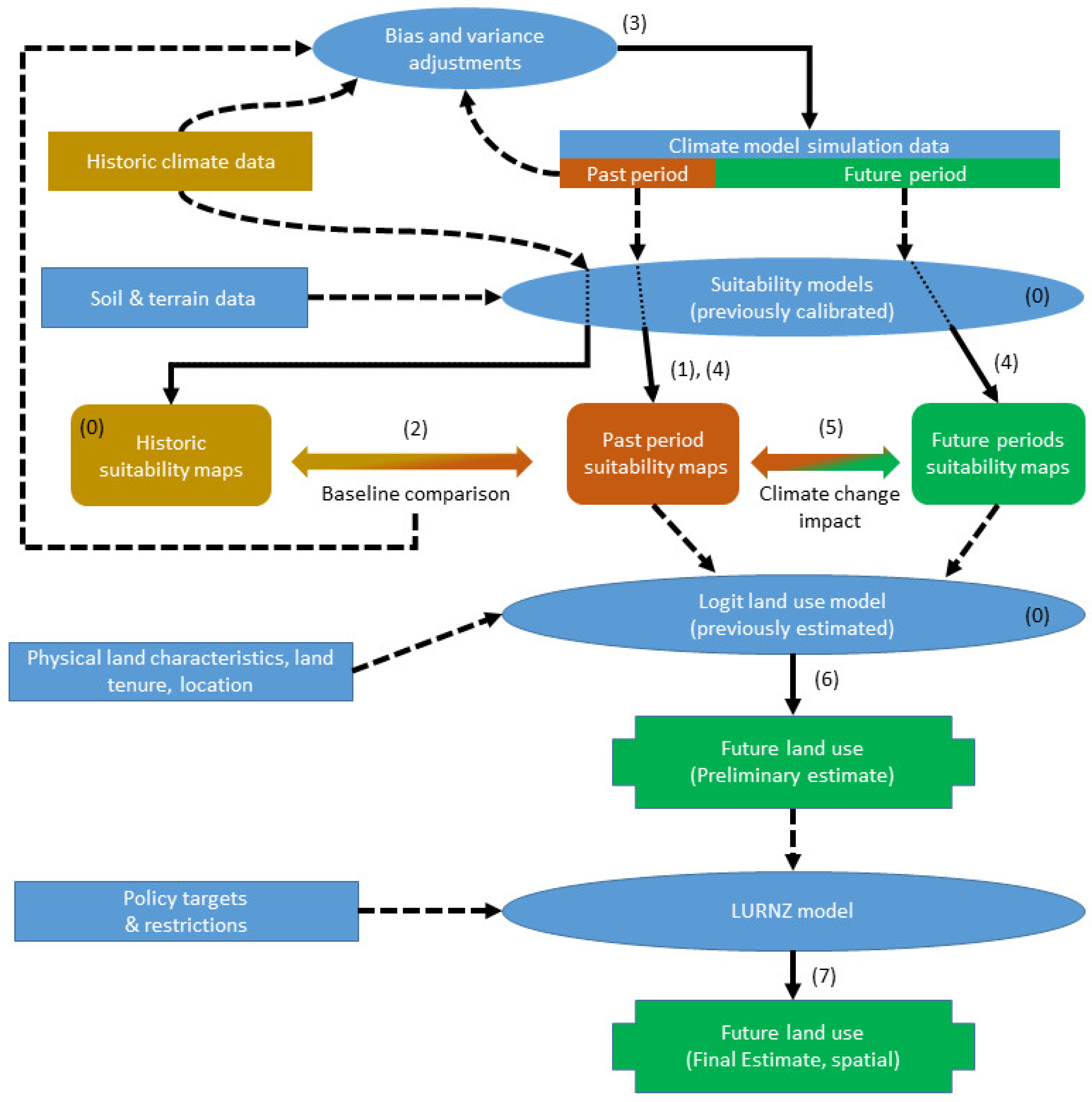
2.1. Models
2.1.1. Continuous Suitability Models
2.1.2. Multinomial Logit Model of Land Use
2.1.3. Land Use in Rural New Zealand Model
2.2. Software
2.3. Data
2.4. Correction to RCP Datasets
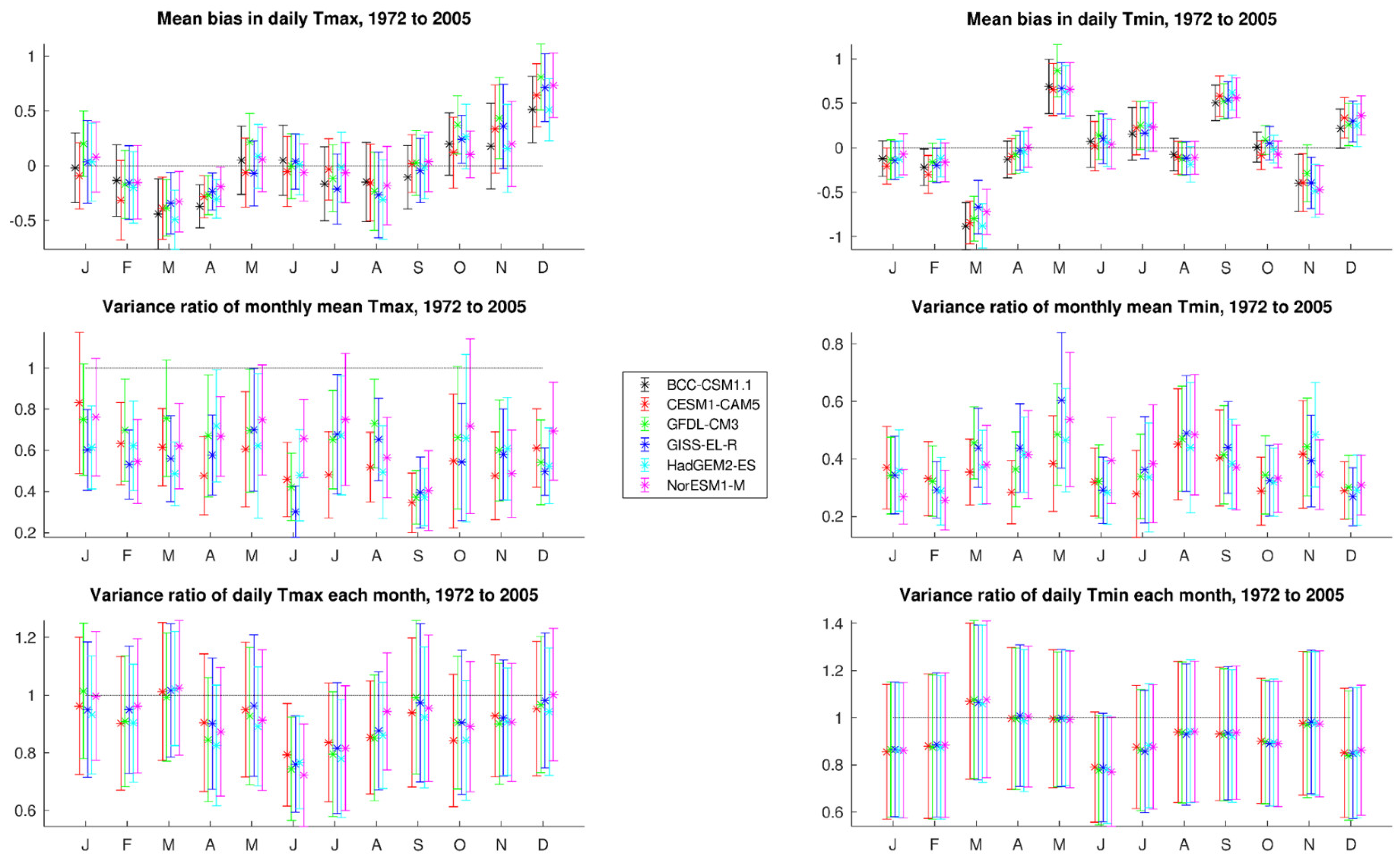
2.4.1. Biases
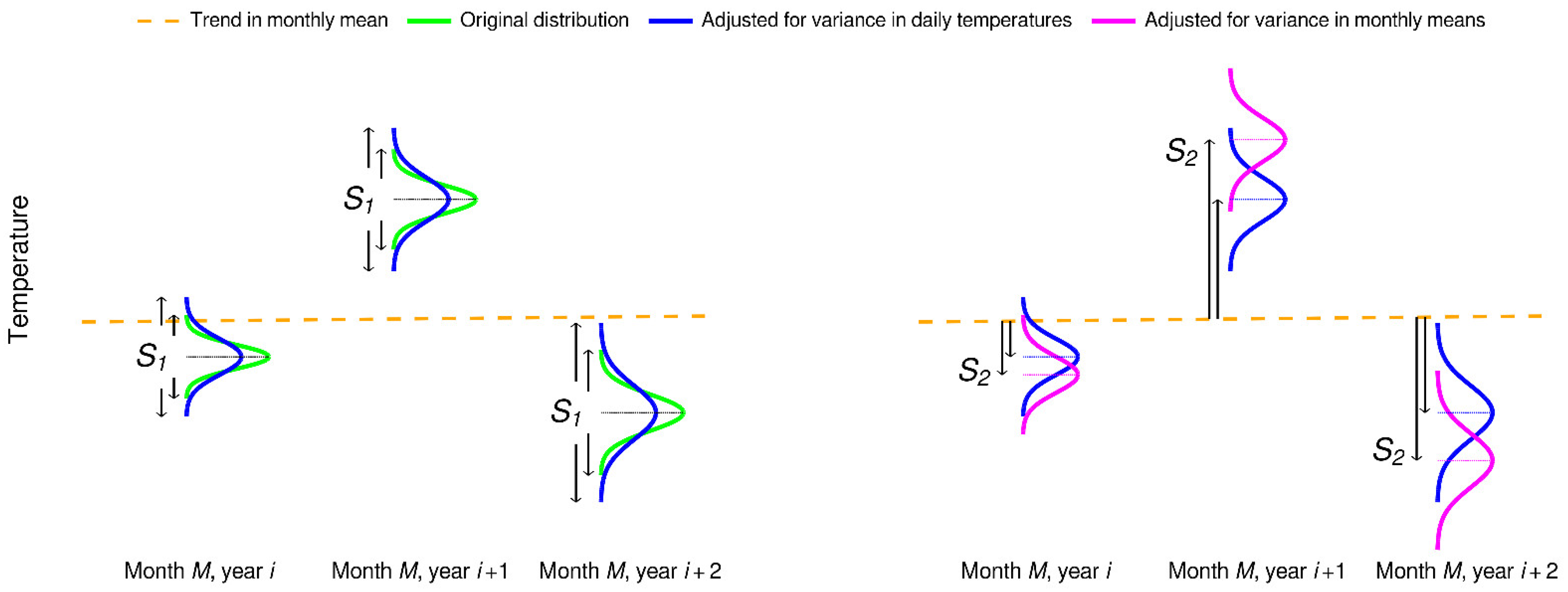
2.4.2. Correction to RCP Datasets to Align Monthly Temperature Statistics
Correcting RCP Past Temperature Datasets
- Adjust for differences between each RCP dataset and the VCSN dataset in the mean variance of daily maximum and minimum temperatures for the month:
- (a)
- is the mean daily maximum or minimum temperature for the month in year
- (b)
- is the standard deviation of the daily (suffix d) RCP (suffix R) maximum or minimum temperature for the month, calculated over the 1972–2005 period using the following formula, with being the number of years and being the number of days in the month for year
- (c)
- is the standard deviation of the daily VCSN (suffix V) temperatures for the month over the same period, calculated by applying an equation analogous to Equation (2) to the VCSN data.
- Adjust for the difference between each RCP dataset and the VCSN dataset in the variation of the monthly mean maximum or minimum temperature around the corresponding monthly mean for the period:where
- (a)
- is the value at year of the spline smooth of the entire 1972–2099 data series.
- (b)
- is the standard deviation of the RCP monthly (suffix m) mean of individual years around , calculated as:where is the mean of for the 1972–2005 period.
- (c)
- is the standard deviation of the VCSN mean (maximum or minimum) temperature for the month over individual years, calculated around the VCSN mean monthly (maximum or minimum) temperature over the 1972–2005 period using an analogous equation to Equation (2).
- Correct for bias with respect to monthly means for the RCP maximum and minimum temperature.
Correcting RCP Future Datasets
2.5. Estimation of Uncertainty in Projections
2.6. Future Location Suitability
2.7. Land-Use Modelling
2.7.1. Integration of Logit Model Results with the LURNZ Model
2.7.2. Climate-Driven Land-Use Change
2.7.3. Economic and Policy Context
2.7.4. Implementation
3. Results
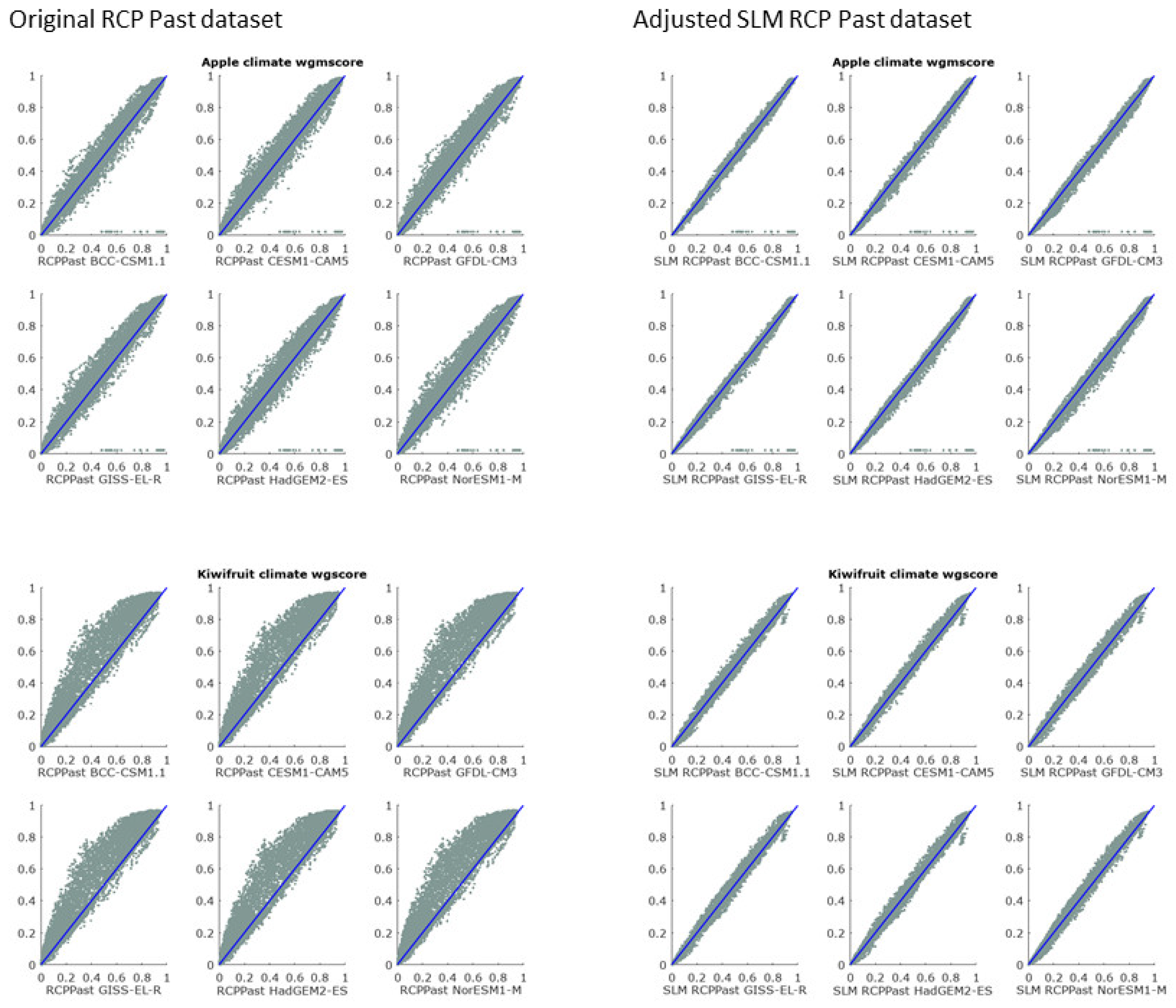
3.1. RCP Data Corrections
3.2. Suitability Projections
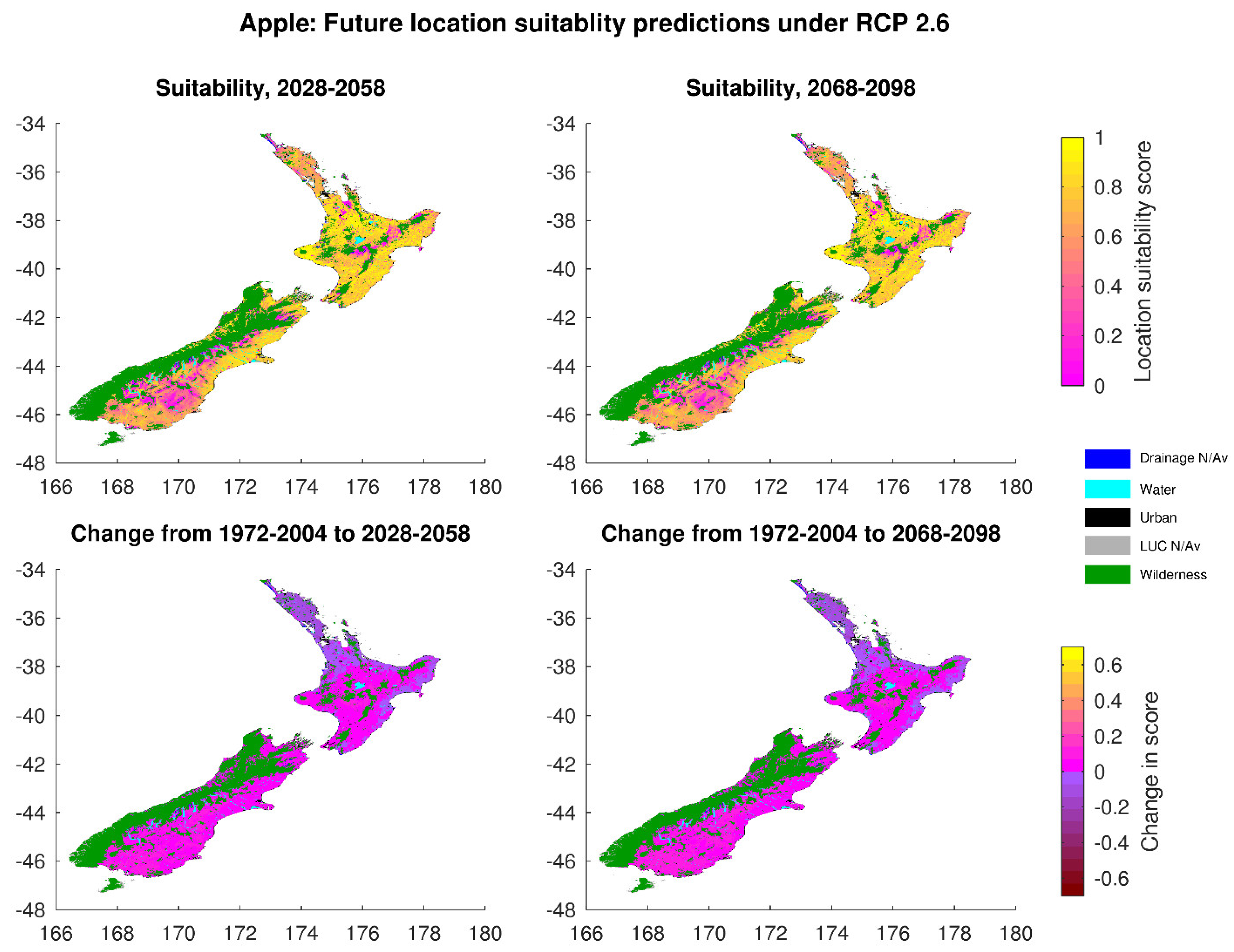
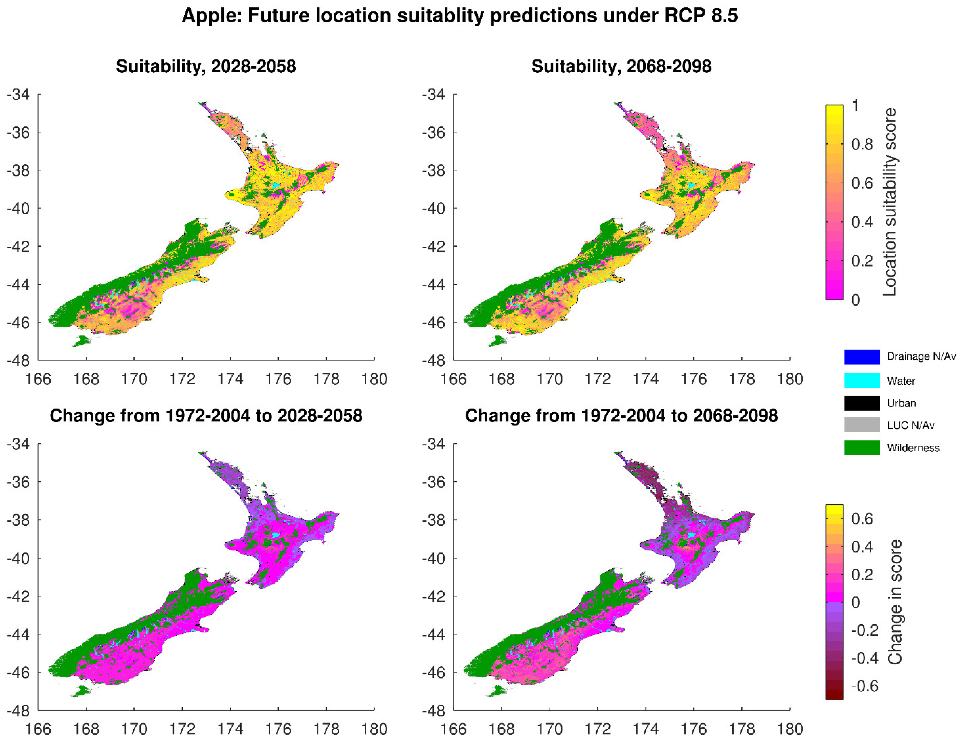
3.2.1. Apple
Apple RCP 2.6
Apple RCP 8.5
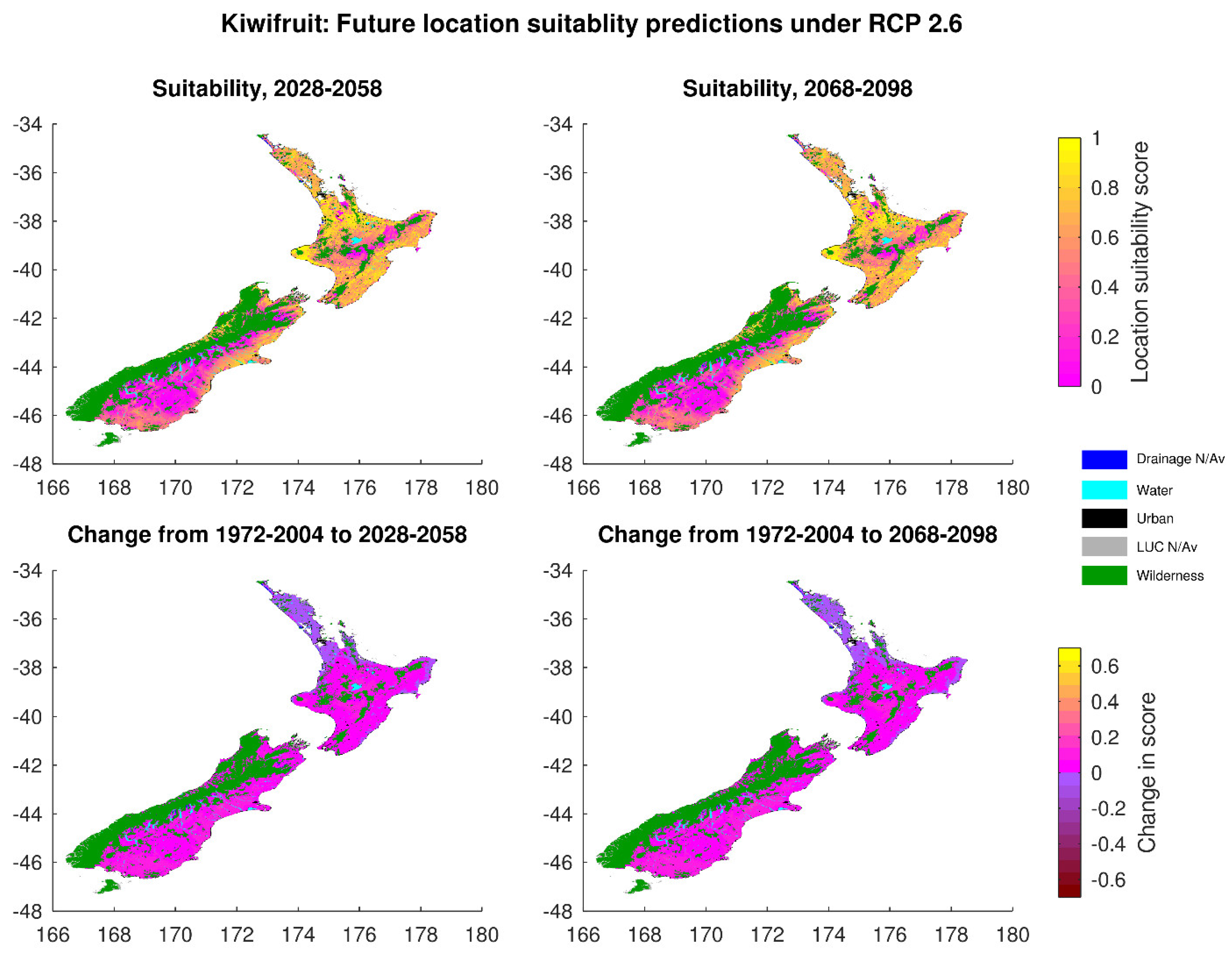
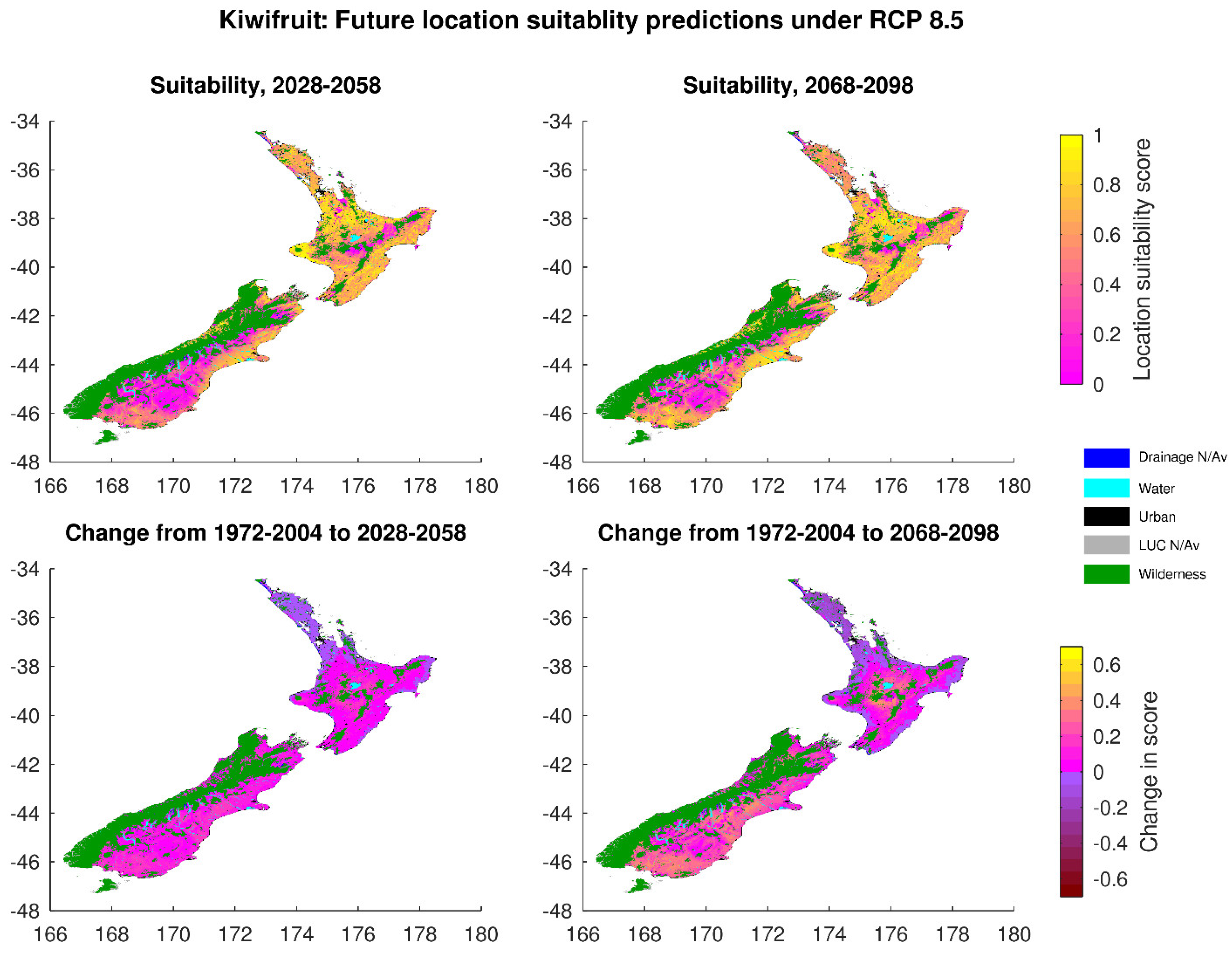
3.2.2. Kiwifruit
Kiwifruit RCP 2.6
Kiwifruit RCP 8.5
3.3. Land Use Change
3.3.1. Multinomial Logit Model Projections
3.3.2. LURNZ Simulations
4. Discussion
4.1. Bias and Variance Corrections to Climate Model Data
4.2. Suitability Projections
4.3. Land-Use Econometric Projections
4.4. Policy Implications
4.5. Limitations and Context with Respect to Other Studies
5. Conclusions
Supplementary Materials
Author Contributions
Funding
Data Availability Statement
Acknowledgments
Conflicts of Interest
Appendix A
A.1. Effect of Bias Adjustments on Climate Change Signals

| Elevations < 500 m | All Elevations | |||||||||||
| Period | 2031–2050 | 2080–2099 | 2031–2050 | 2080–2099 | ||||||||
| LE | UE | LE | UE | |||||||||
| Annual minimum temperature signal impact (°C) | ||||||||||||
| RCP 2.6 | −0.02 | 0.02 | −0.02 | 0.01 | −0.04 | 0.02 | −0.17 | 0.03 | −0.04 | 0.02 | −0.20 | 0.02 |
| RCP 4.5 | −0.03 | 0.00 | −0.03 | 0.01 | −0.06 | 0.00 | −0.19 | 0.01 | −0.05 | 0.01 | −0.17 | 0.01 |
| RCP 6.0 | −0.03 | 0.02 | −0.02 | 0.02 | −0.04 | 0.02 | −0.19 | 0.02 | −0.04 | 0.02 | −0.21 | 0.02 |
| RCP 8.5 | −0.02 | 0.02 | −0.02 | 0.01 | −0.04 | 0.02 | −0.20 | 0.03 | −0.05 | 0.01 | −0.21 | 0.01 |
| Mean annual maximum temperature signal impact (°C) | ||||||||||||
| RCP 2.6 | −0.01 | 0.02 | −0.01 | 0.02 | −0.01 | 0.06 | −0.02 | 0.22 | −0.01 | 0.06 | −0.03 | 0.19 |
| RCP 4.5 | −0.02 | 0.01 | −0.01 | 0.01 | −0.03 | 0.02 | −0.06 | 0.13 | −0.01 | 0.04 | −0.03 | 0.16 |
| RCP 6.0 | −0.01 | 0.01 | −0.01 | 0.02 | −0.01 | 0.04 | −0.02 | 0.18 | −0.01 | 0.06 | −0.03 | 0.21 |
| RCP 8.5 | −0.02 | 0.02 | −0.01 | 0.02 | −0.02 | 0.05 | −0.03 | 0.20 | −0.01 | 0.05 | −0.03 | 0.18 |
| Mean annual mean temperature signal impact (°C) | ||||||||||||
| RCP 2.6 | −0.01 | 0.01 | −0.01 | 0.01 | −0.01 | 0.02 | −0.02 | 0.04 | −0.01 | 0.02 | −0.03 | 0.05 |
| RCP 4.5 | −0.02 | 0.00 | −0.01 | 0.00 | −0.03 | 0.00 | −0.06 | 0.01 | −0.02 | 0.01 | −0.03 | 0.02 |
| RCP 6.0 | −0.02 | 0.01 | −0.01 | 0.01 | −0.02 | 0.01 | −0.04 | 0.03 | −0.01 | 0.02 | −0.03 | 0.03 |
| RCP 8.5 | −0.01 | 0.01 | −0.01 | 0.01 | −0.01 | 0.02 | −0.03 | 0.05 | −0.01 | 0.01 | −0.03 | 0.01 |
| Annual minimum temperature variance ratio signal impact (1) | ||||||||||||
| RCP 2.6 | −0.02 | 0.00 | −0.02 | 0.01 | −0.02 | 0.00 | −0.05 | 0.01 | −0.02 | 0.01 | −0.04 | 0.01 |
| RCP 4.5 | −0.02 | 0.01 | −0.02 | 0.01 | −0.02 | 0.01 | −0.03 | 0.02 | −0.02 | 0.01 | −0.04 | 0.03 |
| RCP 6.0 | −0.02 | 0.01 | −0.03 | 0.02 | −0.02 | 0.01 | −0.05 | 0.01 | −0.03 | 0.02 | −0.05 | 0.03 |
| RCP8.5 | −0.03 | 0.01 | −0.04 | 0.04 | −0.02 | 0.01 | −0.05 | 0.02 | −0.04 | 0.04 | −0.07 | 0.06 |
| Annual maximum temperature variance ratio signal impact (1) | ||||||||||||
| RCP 2.6 | −0.02 | 0.00 | −0.03 | 0.00 | −0.04 | 0.00 | −0.08 | 0.00 | −0.03 | 0.00 | −0.07 | 0.01 |
| RCP 4.5 | −0.02 | 0.01 | −0.03 | 0.01 | −0.03 | 0.01 | −0.08 | 0.02 | −0.05 | 0.01 | −0.09 | 0.02 |
| RCP 6.0 | −0.02 | 0.00 | −0.04 | 0.01 | −0.03 | 0.00 | −0.08 | 0.01 | −0.06 | 0.02 | −0.12 | 0.03 |
| RCP8.5 | −0.02 | 0.01 | −0.05 | 0.02 | −0.04 | 0.01 | −0.10 | 0.02 | −0.07 | 0.03 | −0.15 | 0.05 |
Appendix B
|
Apple SLM RCP 2.6 |
Historic (km2) 1972–2004 |
Area Change from Historic (km2) 2028–2058 |
Area Change from Historic (km2) 2068–2098 | ||||
| Suitability Range | Forecast | Best Case | Worst Case | Forecast | Best Case | Worst Case | |
| 0–0.1 | 14,891 | −1498 | −3175 | 354 | −1603 | −3176 | 83 |
| 0.1–0.2 | 4286 | −828 | −1980 | −673 | −909 | −2126 | −648 |
| 0.2–0.3 | 4972 | −1266 | −617 | −134 | −1404 | −711 | −358 |
| 0.3–0.4 | 8321 | −2494 | −4201 | −367 | −2711 | −4302 | −479 |
| 0.4–0.5 | 12,457 | −2057 | −4464 | 393 | −1947 | −4767 | 582 |
| 0.5–0.6 | 22,444 | −2387 | −6174 | 855 | −2340 | −5949 | 1101 |
| 0.6–0.7 | 31,668 | 3815 | 916 | 4969 | 4474 | 1137 | 5157 |
| 0.7–0.8 | 32,230 | 948 | 3752 | −2846 | 507 | 3689 | −2872 |
| 0.8–0.9 | 31,947 | 4558 | 5270 | 2744 | 5380 | 6011 | 3525 |
| 0.9–1.0 | 20,509 | 1209 | 10,673 | −5295 | 553 | 10,194 | −6091 |
|
Apple SLM RCP 8.5 |
Historic (km2) 1972–2004 |
Area Change from Historic (km2) 2028–2058 |
Area Change from Historic (km2) 2068–2098 | ||||
| Suitability Range | Forecast | Best Case | Worst Case | Forecast | Best Case | Worst Case | |
| 0–0.1 | 14,891 | −2027 | −3173 | −778 | −2803 | −3182 | −2319 |
| 0.1–0.2 | 4286 | −1442 | −2263 | −1235 | −3032 | −3575 | −2289 |
| 0.2–0.3 | 4972 | −1606 | −1245 | −956 | −609 | −2420 | 3118 |
| 0.3–0.4 | 8321 | −3184 | −4552 | −1291 | 2473 | −1186 | 2765 |
| 0.4–0.5 | 12,457 | −2104 | −4868 | 312 | −1299 | −276 | −576 |
| 0.5–0.6 | 22,444 | −2675 | −5170 | 481 | −2841 | −6048 | −320 |
| 0.6–0.7 | 31,668 | 3690 | 887 | 4116 | 1518 | 420 | 2898 |
| 0.7–0.8 | 32,230 | 886 | 3221 | −1587 | 2695 | 516 | 3576 |
| 0.8–0.9 | 31,947 | 8143 | 9460 | 5662 | 14,150 | 19,873 | 7711 |
| 0.9–1.0 | 20,509 | 319 | 7703 | −4724 | −10,252 | −4122 | −14,564 |
|
Kiwifruit SLM RCP 2.6 |
Historic (km2) 1972–2004 |
Area Change from Historic (km2) 2028–2058 |
Area Change from Historic (km2) 2068–2098 | ||||
| Suitability Range | Forecast | Best Case | Worst Case | Forecast | Best Case | Worst Case | |
| 0–0.1 | 37,541 | −6215 | −13,048 | −1090 | −6716 | −13,358 | −1591 |
| 0.1–0.2 | 12,757 | −1983 | 475 | −3079 | −2080 | 256 | −3287 |
| 0.2–0.3 | 14,845 | −2929 | −2971 | −1100 | −3176 | −3311 | −1417 |
| 0.3–0.4 | 16,808 | −1861 | −2746 | −1457 | −1891 | −2890 | −1636 |
| 0.4–0.5 | 19,596 | 1515 | −698 | 3121 | 1578 | −677 | 3637 |
| 0.5–0.6 | 21,305 | 2873 | 3919 | 1477 | 3035 | 3968 | 1774 |
| 0.6–0.7 | 19,058 | 4377 | 4089 | 3680 | 4988 | 4894 | 4079 |
| 0.7–0.8 | 18,653 | 763 | 2778 | −1107 | 784 | 2765 | −956 |
| 0.8–0.9 | 16,787 | 2604 | 3936 | 586 | 2884 | 4414 | 698 |
| 0.9–1.0 | 6375 | 856 | 4266 | −1031 | 594 | 3939 | −1301 |
|
Kiwifruit SLM RCP 8.5 |
Historic (km2) 1972–2004 |
Area Change from Historic (km2) 2028–2058 |
Area Change from Historic (km2) 2068–2098 | ||||
| Suitability Range | Forecast | Best Case | Worst Case | Forecast | Best Case | Worst Case | |
| 0–0.1 | 37,541 | −9686 | −14,697 | −4759 | −17,463 | −19,709 | −15,442 |
| 0.1–0.2 | 12,757 | −2002 | −889 | −4351 | −5839 | −6114 | −5716 |
| 0.2–0.3 | 14,845 | −4198 | −3394 | −3249 | −5741 | −5724 | −5195 |
| 0.3–0.4 | 16,808 | −2418 | −3948 | −1778 | −5228 | −5849 | −3959 |
| 0.4–0.5 | 19,596 | 383 | −613 | 2948 | 338 | −1100 | 1939 |
| 0.5–0.6 | 21,305 | 4372 | 3953 | 3224 | 6462 | 4249 | 7256 |
| 0.6–0.7 | 19,058 | 6768 | 6813 | 5570 | 7760 | 8058 | 7735 |
| 0.7–0.8 | 18,653 | 1655 | 3830 | 706 | 10,464 | 10,312 | 9672 |
| 0.8–0.9 | 16,787 | 3650 | 5184 | 1842 | 9716 | 13,421 | 5911 |
| 0.9–1.0 | 6375 | 1476 | 3761 | −153 | −469 | 2456 | −2201 |
References
- Manning, M.; Lawrence, J.; King, D.N.; Chapman, R. Dealing with changing risks: A New Zealand perspective on climate change adaptation. Reg. Environ. Chang. 2015, 15, 581–594. [Google Scholar] [CrossRef]
- Clothier, B.; Hall, A.; Green, S. Adapting the horticultural and vegetable industries to climate change. In Impacts of Climate Change on Land-Based Sectors and Adaptation Options; Clark, A., Nottage, R., Eds.; MPI Technical Paper No: 2012/33; The Ministry of Primary Industry: Wellington, New Zealand, 2012; pp. 237–292. [Google Scholar]
- Hatfield, J.L.; Prueger, J.H. Temperature extremes: Effect on plant growth and development. Weather. Clim. Extrem. 2015, 10, 4–10. [Google Scholar] [CrossRef]
- Snyder, R. Climate change impacts on water use in horticulture. Horticulturae 2017, 3, 27. [Google Scholar] [CrossRef]
- Jones, R. Future scenarios for plant virus pathogens as climate change progresses. Adv. Virus Res. 2016, 95, 87–147. [Google Scholar] [PubMed]
- Trębicki, P.; Dáder, B.; Vassiliadis, S.; Fereres, A. Insect–plant–pathogen interactions as shaped by future climate: Effects on biology, distribution, and implications for agriculture. Insect Sci. 2017, 24, 975–989. [Google Scholar] [CrossRef]
- Wakelin, S.A.; Gomez-Gallego, M.; Jones, E.; Smaill, S.; Lear, G.; Lambie, S. Climate change induced drought impacts on plant diseases in New Zealand. Australas. Plant Pathol. 2018, 47, 101–114. [Google Scholar] [CrossRef]
- Warrick, R.A.; Kenny, G.J.; Harman, J.J. The Effects of Climate Change and Variation in New Zealand: An Assessment Using the CLIMPACTS System; The International Global Change Institute (IGCI), University of Waikato: Hamilton, New Zealand, 2001. [Google Scholar]
- Hall, A.; Stanley, J.; Müller, K.; van den Dijssel, C. Criteria for Defining Climatic Suitability of Horticultural Crops; Client Report for the Ministry for Primary Industries; Plant & Food Research: Auckland, New Zealand, 2018. [Google Scholar]
- Cradock-Henry, N.A.; Blackett, P.; Hall, M.; Johnstone, P.; Teixeira, E.; Wreford, A. Climate adaptation pathways for agriculture: Insights from a participatory process. Environ. Sci. Policy 2020, 107, 66–79. [Google Scholar] [CrossRef]
- Zheng, Q.; Siman, K.; Zeng, Y.; Teo, H.C.; Sarira, T.V.; Sreekar, R.; Koh, L.P. Future land-use competition constrains natural climate solutions. Sci. Total Environ. 2022, 838, 156409. [Google Scholar] [CrossRef] [PubMed]
- Xu, Y.; Yao, L. Integrating Climate Change Adaptation and Mitigation into Land Use Optimization: A Case Study in Huailai County, China. Land 2021, 10, 1297. [Google Scholar] [CrossRef]
- Abd-Elmabod, S.K.; Muñoz-Rojas, M.; Jordán, A.; Anaya-Romero, M.; Phillips, J.D.; Jones, L.; Zhang, Z.; Pereira, P.; Fleskens, L.; van der Ploeg, M.; et al. Climate change impacts on agricultural suitability and yield reduction in a Mediterranean region. Geoderma 2020, 374, 114453. [Google Scholar] [CrossRef]
- Gardner, A.S.; Maclean, I.M.D.; Gaston, K.J.; Bütikofer, L. Forecasting future crop suitability with microclimate data. Agric. Syst. 2021, 190, 103084. [Google Scholar] [CrossRef]
- Gebrehiwot, A.A.; Hashemi-Beni, L.; Kurkalova, L.A.; Liang, C.L.; Jha, M.K. Using ABM to Study the Potential of Land Use Change for Mitigation of Food Deserts. Sustainability 2022, 14, 9715. [Google Scholar] [CrossRef]
- Cronin, J.; Zabel, F.; Dessens, O.; Anandarajah, G. Land suitability for energy crops under scenarios of climate change and land-use. GCB Bioenergy 2020, 12, 648–665. [Google Scholar] [CrossRef]
- Li, X.; Chen, G.; Liu, X.; Liang, X.; Wang, S.; Chen, Y.; Pei, F.; Xu, X. A new global land-use and land-cover change product at a 1-km resolution for 2010 to 2100 based on human–environment interactions. Ann. Am. Assoc. Geogr. 2017, 107, 1040–1059. [Google Scholar] [CrossRef]
- Truong, Q.C.; Gaudou, B.; Danh, M.V.; Huynh, N.Q.; Drogoul, A.; Taillandier, P. A land-use change model to study climate change adaptation strategies in the Mekong Delta. In Proceedings of the 2021 RIVF International Conference on Computing and Communication Technologies (RIVF), Hanoi, Vietnam, 19–21 August 2021; pp. 1–6. [Google Scholar]
- Glenn, M.; Kim, S.-H.; Ramirez-Villegas, J.; Laderach, P. Response of perennial horticultural crops to climate change. Hort. Rev. 2013, 41, 47–130. [Google Scholar]
- Akpoti, K.; Kabo-bah, A.T.; Zwart, S.J. Review—Agricultural land suitability analysis: State-of-the-art and outlooks for integration of climate change analysis. Agric. Syst. 2019, 173, 172–208. [Google Scholar] [CrossRef]
- Schönhart, M.; Trautvetter, H.; Parajka, J.; Blaschke, A.P.; Hepp, G.; Kirchner, M.; Mitter, H.; Schmid, E.; Strenn, B.; Zessner, M. Modelled impacts of policies and climate change on land use and water quality in Austria. Land Use Policy 2018, 76, 500–514. [Google Scholar] [CrossRef]
- Tait, A.; Paul, V.; Sood, A.; Mowat, A. Potential impact of climate change on Hayward kiwifruit production viability in New Zealand. N. Z. J. Crop Hortic. Sci. 2018, 46, 175–197. [Google Scholar] [CrossRef]
- Vetharaniam, I.; Müller, K.; Stanley, C.J.; van den Dijssel, C.; Timar, L.; Clothier, B. Modelling continuous location suitability scores and spatial footprint of apple and kiwifruit in New Zealand. Land 2022, 11, 1528. [Google Scholar] [CrossRef]
- Kerr, S.; Anastasiadis, S.; Olssen, A.; Power, W.; Timar, L.; Zhang, W. Spatial and temporal responses to an emissions trading scheme covering agriculture and forestry: Simulation results from New Zealand. Forests 2012, 3, 1133–1156. [Google Scholar] [CrossRef]
- Ministry for the Environment. Climate Change Projections for New Zealand: Atmosphere Projections Based on Simulations from the IPCC Fifth Assessment, 2nd ed.; Ministry for the Environment: Wellington, New Zealand, 2018. [Google Scholar]
- Challinor, A.J.; Müller, C.; Asseng, S.; Deva, C.; Nicklin, K.J.; Wallach, D.; Vanuytrecht, E.; Whitfield, S.; Ramirez-Villegas, J.; Koehler, A.-K. Improving the use of crop models for risk assessment and climate change adaptation. Agric. Syst. 2018, 159, 296–306. [Google Scholar] [CrossRef] [PubMed]
- Maraun, D. Bias correcting climate change simulations-a critical review. Curr. Clim. Chang. Rep. 2016, 2, 211–220. [Google Scholar] [CrossRef]
- Kidd, D.; Webb, M.; Malone, B.; Minasny, B.; McBratney, A. Digital soil assessment of agricultural suitability, versatility and capital in Tasmania, Australia. Geoderma Reg. 2015, 6, 7–21. [Google Scholar] [CrossRef]
- Timar, L. Rural Land Use and Land Tenure in New Zealand; Motu Economic and Public Policy Research: Wellington, New Zealand, 2011. [Google Scholar]
- Blackman, A.; Albers, H.J.; Ávalos-Sartorio, B.; Murphy, L.C. Land cover in a managed forest ecosystem: Mexican shade coffee. Am. J. Agric. Econ. 2008, 90, 216–231. [Google Scholar] [CrossRef]
- Chomitz, K.M.; Gray, D.A. Roads, land use, and deforestation: A spatial model applied to Belize. World Bank Econ. Rev. 1996, 10, 487–512. [Google Scholar] [CrossRef]
- Lubowski, R.N.; Plantinga, A.J.; Stavins, R.N. What drives land-use change in the United States? A national analysis of landowner decisions. Land Econ. 2008, 84, 529–550. [Google Scholar] [CrossRef]
- Kerr, S.; Olssen, A. Gradual Land-Use Change in New Zealand: Results from a Dynamic Econometric Model; Motu Economic and Public Policy Research: Wellington, New Zealand, 2012. [Google Scholar]
- Timar, L. Yield to Change: Modelling the Land-Use Response to Climate-Driven Changes in Pasture Production; Motu Economic and Public Policy Research: Wellington, New Zealand, 2016. [Google Scholar]
- Anastasiadis, S.; Kerr, S.; Zhang, W.; Allan, C.; Power, W. Land Use in Rural New Zealand: Spatial Land Use, Land-Use Change, and Model Validation. Available online: https://ageconsearch.umn.edu/record/189507/files/Anastasiadis_etal_2013.pdf (accessed on 10 April 2020).
- Timar, L.; Kerr, S. Land-Use Intensity and Greenhouse Gas Emissions in the LURNZ Model; Motu Economic and Public Policy Research: Wellington, New Zealand, 2014. [Google Scholar]
- Parliamentary Commissioner for the Environment. Farms, Forests and Fossil Fuels: The Next Great Landscape Transformation? Parliamentary Commissioner for the Environment: Wellington, New Zealand, 2019. [Google Scholar]
- Buis, A. Study Confirms Climate Models Are Getting Future Warming Projections Right. Available online: https://climate.nasa.gov/news/2943/study-confirms-climate-models-are-getting-future-warming-projections-right/ (accessed on 12 January 2021).
- Productivity Commission. Low-Emissions Economy: Final Report; Productivity Commission: Wellington, New Zealand, 2018. [Google Scholar]
- Ministry for the Environment. National Policy Statement for Freshwater Management 2014 (Amended 2017). Available online: https://www.mfe.govt.nz/publications/fresh-water/national-policy-statement-freshwater-management-2014-amended-2017 (accessed on 7 June 2021).
- Kenny, G. Climate Change: Likely Impacts on New Zealand Agriculture; Ministry for the Environment: Wellington, New Zealand, 2001. [Google Scholar]
- Pearce, P. Northland Climate Change Projections and Impacts; Client Report for Northland Regional Council, New Zealand National Institute of Water and Atmospheric Research: Wellington, New Zealand, 2017. [Google Scholar]
- Wang, S.; Huang, C.; Tao, J.; Zhong, M.; Qu, X.; Wu, H.; Xu, X. Evaluation of chilling requirement of kiwifruit (Actinidia spp.) in south China. N. Z. J. Crop Hortic. Sci. 2017, 45, 289–298. [Google Scholar] [CrossRef]
- Zhao, T.; Li, D.; Li, L.; Han, F.; Liu, X.; Zhang, P.; Chen, M.; Zhong, C. The differentiation of chilling requirements of kiwifruit cultivars related to ploidy variation. HortScience 2017, 52, 1676. [Google Scholar] [CrossRef]
- Hall, A.J.; Kenny, G.J.; Austin, P.T.; McPherson, H.G. Changes in kiwifruit phenology with climate. In The Effects of Climate Change and Variation in New Zealand: An Assessment Using the CLIMPACTS System; Warrick, R.A., Kenny, G.J., Harman, J.J., Eds.; International Global Change Institute (IGCI), University of Waikato: Hamilton, New Zealand, 2001; pp. 33–46. [Google Scholar]
- Austin, P.T.; Hall, A.J. Temperature impacts on development of apple fruits. In The Effects of Climate Change and Variation in New Zealand: An Assessment Using the CLIMPACTS System; Warrick, R.A., Kenny, G.J., Harman, J.J., Eds.; International Global Change Institute (IGCI), University of Waikato: Hamilton, New Zealand, 2001; pp. 47–55. [Google Scholar]
- Singh, M.; Bathia, H. Thermal indices in relation to crop phenology and fruit yield of apple. Mausam 2012, 63, 449–454. [Google Scholar] [CrossRef]
- Sugiura, T.; Kuroda, H.; Sugiura, H.; Honjo, H. Prediction of effects of global warming on apple production regions in Japan. Phyton Ann. Rei Bot. 2005, 45, 419–422. [Google Scholar]
- Zabel, F.; Putzenlechner, B.; Mauser, W. Global agricultural land resources–a high resolution suitability evaluation and its perspectives until 2100 under climate change conditions. PLoS ONE 2014, 9, e107522. [Google Scholar] [CrossRef] [PubMed]
- Doelman, J.C.; Stehfest, E.; Tabeau, A.; van Meijl, H.; Lassaletta, L.; Gernaat, D.E.H.J.; Hermans, K.; Harmsen, M.; Daioglou, V.; Biemans, H.; et al. Exploring SSP land-use dynamics using the IMAGE model: Regional and gridded scenarios of land-use change and land-based climate change mitigation. Glob. Environ. Chang. 2018, 48, 119–135. [Google Scholar] [CrossRef] [Green Version]
- Vetharaniam, I.; Müller, K.; Stanley, J.; van den Dijssel, C.; Timar, L.; Cummins, M. Modelling the Effect of Climate Change on Land Suitability for Growing Perennial Crops; Plant & Food Research Ltd.: Auckland, New Zealand, 2021. [Google Scholar]

| Land Use | RCP 2.6 Mid | RCP 2.6 Late | RCP 8.5 Mid | RCP 8.5 Late |
|---|---|---|---|---|
| Kiwifruit | 1875 | 1825 | 2675 | 3800 |
| Apple | 150 | 125 | 100 | −1050 |
| Land Use | Basemap | 2030 | 2045 | 2060 | 2075 |
|---|---|---|---|---|---|
| Kiwifruit | 15,600 | 15,750 | 16,550 | 17,350 | 17,475 |
| Apple | 9425 | 9425 | 9500 | 9550 | 9575 |
| Other horticulture | 447,450 | 447,425 | 447,075 | 446,800 | 446,775 |
| Dairy | 2,098,200 | 2,291,375 | 2,290,925 | 2,290,500 | 2,290,450 |
| Sheep–beef | 8,152,825 | 7,488,125 | 7,243,025 | 6,916,975 | 6,685,075 |
| Forestry | 2,002,075 | 2,426,775 | 2,894,325 | 3,387,875 | 3,687,350 |
| Scrub | 1,743,000 | 1,789,700 | 1,567,175 | 1,399,525 | 1,331,875 |
| Land Use | Basemap | 2030 | 2045 | 2060 | 2075 |
|---|---|---|---|---|---|
| Kiwifruit | 15,600 | 15,825 | 16,975 | 18,375 | 18,675 |
| Apple | 9425 | 9425 | 9475 | 425 | 9125 |
| Other horticulture | 447,450 | 447,400 | 446,950 | 446,550 | 446,850 |
| Dairy | 2,098,200 | 2,291,325 | 2,290,750 | 2,290,050 | 2,290,025 |
| Sheep–beef | 8,152,825 | 7,488,025 | 7,242,575 | 6,823,850 | 6,683,325 |
| Forestry | 2,002,075 | 2,426,775 | 2,894,300 | 3,508,800 | 3,687,300 |
| Scrub | 1,743,000 | 1,789,800 | 1,567,550 | 1,371,525 | 1,333,275 |
| RCP 2.6 | RCP 8.5 | ||||||
|---|---|---|---|---|---|---|---|
| Region | Basemap | Loss | Gain | 2075 | Loss | Gain | 2075 |
| Auckland | 375 | 50 | 0 | 325 | 200 | 0 | 175 |
| Bay of Plenty | 11,625 | 650 | 75 | 11,050 | 4275 | 75 | 7425 |
| Canterbury | 0 | 0 | 0 | 0 | 0 | 1625 | 1625 |
| Gisborne | 600 | 25 | 25 | 600 | 125 | 150 | 625 |
| Hawkes Bay | 350 | 0 | 325 | 675 | 0 | 2325 | 2675 |
| Manawatu-Wanganui | 100 | 0 | 0 | 100 | 0 | 0 | 100 |
| Marlborough | 0 | 0 | 0 | 0 | 0 | 950 | 950 |
| Nelson | 0 | 0 | 0 | 0 | 0 | 50 | 50 |
| Northland | 1000 | 225 | 0 | 775 | 600 | 0 | 400 |
| Otago | 0 | 0 | 0 | 0 | 0 | 400 | 400 |
| Southland | 0 | 0 | 0 | 0 | 0 | 0 | 0 |
| Taranaki | 0 | 0 | 2425 | 2425 | 0 | 2275 | 2275 |
| Tasman | 700 | 0 | 0 | 700 | 0 | 625 | 1325 |
| Waikato | 825 | 25 | 0 | 800 | 225 | 0 | 600 |
| Wellington | 0 | 0 | 0 | 0 | 0 | 25 | 25 |
| West Coast | 0 | 0 | 0 | 0 | 0 | 0 | 0 |
| Outside RC boundaries | 25 | 0 | 0 | 25 | 0 | 0 | 25 |
| Total | 15,600 | 975 | 2850 | 17,475 | 5425 | 8500 | 18,675 |
| RCP 2.6 | RCP 8.5 | ||||||
|---|---|---|---|---|---|---|---|
| Region | Basemap | Loss | Gain | 2075 | Loss | Gain | 2075 |
| Auckland | 75 | 0 | 0 | 75 | 50 | 0 | 25 |
| Bay of Plenty | 0 | 0 | 0 | 0 | 0 | 0 | 0 |
| Canterbury | 50 | 0 | 50 | 100 | 0 | 875 | 925 |
| Gisborne | 150 | 0 | 25 | 175 | 50 | 25 | 125 |
| Hawkes Bay | 5900 | 175 | 125 | 5850 | 1600 | 25 | 4325 |
| Manawatu-Wanganui | 0 | 0 | 0 | 0 | 0 | 0 | 0 |
| Marlborough | 0 | 0 | 0 | 0 | 0 | 0 | 0 |
| Nelson | 0 | 0 | 0 | 0 | 0 | 0 | 0 |
| Northland | 0 | 0 | 0 | 0 | 0 | 0 | 0 |
| Otago | 725 | 0 | 0 | 725 | 0 | 525 | 1250 |
| Southland | 0 | 0 | 0 | 0 | 0 | 0 | 0 |
| Taranaki | 0 | 0 | 125 | 125 | 0 | 75 | 75 |
| Tasman | 2250 | 0 | 0 | 2250 | 50 | 0 | 2200 |
| Waikato | 150 | 0 | 0 | 150 | 50 | 0 | 100 |
| Wellington | 100 | 0 | 0 | 100 | 25 | 0 | 75 |
| West Coast | 0 | 0 | 0 | 0 | 0 | 0 | 0 |
| Outside RC boundaries | 25 | 0 | 0 | 25 | 0 | 0 | 25 |
| Total | 9425 | 175 | 325 | 9575 | 1825 | 1525 | 9125 |
Publisher’s Note: MDPI stays neutral with regard to jurisdictional claims in published maps and institutional affiliations. |
© 2022 by the authors. Licensee MDPI, Basel, Switzerland. This article is an open access article distributed under the terms and conditions of the Creative Commons Attribution (CC BY) license (https://creativecommons.org/licenses/by/4.0/).
Share and Cite
Vetharaniam, I.; Timar, L.; Stanley, C.J.; Müller, K.; van den Dijssel, C.; Clothier, B. Modelling Climate Change Impacts on Location Suitability and Spatial Footprint of Apple and Kiwifruit. Land 2022, 11, 1639. https://doi.org/10.3390/land11101639
Vetharaniam I, Timar L, Stanley CJ, Müller K, van den Dijssel C, Clothier B. Modelling Climate Change Impacts on Location Suitability and Spatial Footprint of Apple and Kiwifruit. Land. 2022; 11(10):1639. https://doi.org/10.3390/land11101639
Chicago/Turabian StyleVetharaniam, Indrakumar, Levente Timar, C. Jill Stanley, Karin Müller, Carlo van den Dijssel, and Brent Clothier. 2022. "Modelling Climate Change Impacts on Location Suitability and Spatial Footprint of Apple and Kiwifruit" Land 11, no. 10: 1639. https://doi.org/10.3390/land11101639