Construction and Optimization of the Ecological Security Pattern in Liyang, China

Abstract

Rapid urbanization with unreasonable human disturbances has caused a serious ecological crisis. By constructing an ecological-security pattern (ESP), key landscape elements can be effectively identified. ESP optimization helps to improve a city’s ecosystem services and achieve the harmonious development between man and nature. Therefore, it is crucial to construct an accurate ESP and propose practical ESP optimization strategies. Taking Liyang City as an example, this paper first constructed the ESP with a combination methodology of circuit theory, graph theory, the granularity-reverse method, and the comprehensive-evaluation method. Then, strategies for ESP optimization were proposed in terms of ecological restoration and ecological source promotion. Finally, the optimized ESP was verified by quantitative assessment involving landscape connectivity and network structure. Research results show that the current ESP includes 24 ecological sources, 41 ecological corridors, and 50 ecological nodes that need ecological restoration. In the optimized ESP, 31.5 km² of ecological land is added, 3 ecological sources are added, 55 ecological corridors are generated, and the number of nodes in the ecological network is increased by 4. By comparing the evaluation results before and after optimization, it can be seen that the optimization scheme has a positive effect on landscape connectivity and ecological coordination of the whole region.

1. Introduction

Since the 20th century, human society has entered a stage of rapid urbanization with high-intensity land development, overuse of natural resources, and excessive discharge of pollutants. These unreasonable human disturbances have broken the ecological balance, triggering ecological problems such as global climate change, environmental-capacity shrinkage, biodiversity decrease, and soil loss [1,2], which directly affect the sustainability of regional landscape patterns [3,4], as well as economic competition and national security in the context of globalization [5,6,7,8]. To address these impacts, a variety of international initiatives has been proposed and implemented. The Man and the Biosphere (MAB) program was launched in 1971 by UNESCO and aims to foster interdisciplinary research centered on solving practical problems of people and their environments [9]. The United Nations Environment Programme (UNEP) was established in 1972 and has been the global authority that sets the environmental agenda, provides leadership, and develops solutions on a wide range of environmental issues [10]. A series of multilateral environmental agreements have been put forward, such as the Convention on Biological Diversity (CBD) and the United Nations Framework Convention on Climate Change (UNFCCC) [11,12].

On the practical level of ecological environment governance, the national state has been an active scale. Western democracies led the first wave of national programs addressing the ecological problems from the last third of the 20th century, and developing countries made the second wave of national programs in the late 1980s [13]. By now, most countries in the world have built administrative and technical capacity in land management and environmental protection to respond to the ecological crisis. Sweden has always been an international pioneer in environmental policy. In 1976, it became the first country in the world to establish an agency for nature protection, and two years later came the first piece of environmental legislation, the Environmental Protection Act [14]. The U.S. EPA published the guidance for Ecological Risk Assessment (ERA) in the 1990s, and ERA has become an important component of environment management in the United States, which is a flexible process to evaluate the likelihood of adverse ecological effects from environmental stressors [15]. The U.K. took “landscape” as a notion in spatial planning in the 1970s, and “Landscape Character Assessment Guidance for England and Scotland” was published in 2002 [16]. Since then, the LCA (Landscape Character Assessment) method has been extensively used as a guiding tool for decision-making on land(scape) management [17]. In Germany, the concept of greenways was established to prevent urban sprawl at the beginning of the 20th century and developed into the concept of habitat networks in the 1980s [18]. The nationwide project “Lebensraumkorridore für Mensch und Natur” (“Habitat Corridors for Man and Nature”) was drafted in 2004, proposing an integrated approach to preserving, restoring, and developing ecological interrelationships that maintain species diversity and areas for human use [19]. In the Czech Republic, the concept of the Territorial System of Ecological Stability (TSES) was developed in the mid-1980s and is a part of the environmental legislation [20]. The TSES aims at the ecologically optimal use of the landscape, with the methodology of designing a system of biocenters, biocorridors, and interaction elements hierarchically arranged within biogeographical units [21]. The TSES projects are integral parts of spatial planning for open landscape, forest, and urban areas at the supra-regional, the regional, and the local level [22].

As a large developing country with a complex and fragile ecological background, China has been facing far more serious ecological problems than Western countries. It is more relevant and urgent for China to build a framework for bottom-line ecological system management. The concept of an ecological security pattern (ESP) was first put forward by Kongjian Yu in 1996 and defined as the potential spatial pattern composed of strategic portions and positions of the landscape that have critical significance in safeguarding and controlling certain ecological processes [23]. ESP was proposed as one of the three strategic objectives in the report of the 18th CPC National Congress in 2012. The Fifth Plenary Session of the 18th Central Committee further stated that it is necessary to adhere to green development, make use of nature properly, and build a scientific and reasonable ecological-security pattern. With the Fifth Plenary Session of the 19th Central Committee in 2020 clearly offering to optimize the spatial layout of territory, building a scientific and reasonable ESP has become the basic premise for city construction and social development in China. With the analysis and simulation of landscape processes (the expansion of the city, the spatial movement of species, the flow of water and wind, the diffusion of disasters, etc.), ESP is implemented to determine key landscape elements and important spatial locations and connections [24]. The construction of an ecological-security pattern can help regulate ecological processes and allocate natural resources, and has become an effective spatial way of alleviating the contradiction between ecological protection and economic development [8,25].

In the past 30 years, the related research has experienced a rapid development stage from qualitative description to quantitative analysis, from static evaluation to dynamic simulation, and has become scale diversification and method integration. It has developed from focusing on single-species protection to dealing with comprehensive ecological problems with many objectives. Theoretical methods such as minimum cumulative-resistance modelling, graph theory, and circuit theory are commonly used in ESP studies. A typical research paradigm of “ecological source identification–resistance-surface construction–corridor extraction” has been formed. In terms of source identification, the traditional method is to directly select the core areas of nature reserves or other important ecological land as ecological sources, which is simple and easy to carry out, but lacks ecological needs. The other method of comprehensive evaluation has been widely adopted. The evaluation system should include the evaluation of ecological conditions in the study and the evaluation of the patches. As to the evaluation of ecological conditions, the evaluation indicators are usually selected for ecological sensitivity, ecological carrying capacity, ecosystem services, etc. [15,26,27]. For evaluation of the patches themselves, some scholars are inclined to the patch importance of connectivity [28,29,30]. MSPA (morphological spatial-pattern analysis), a morphology-based pattern-analysis method, is also applied to extract the core and islet in MSPA as ecological spaces that can serve as habitats for species [31,32]. It should be noted that different granularities can cause differences in landscape composition within the same area. To ensure the optimal landscape structure, some scholars have explored the variation characteristics of landscape-component structure with different granularities. The granularity-reverse method is used in some research to determine the optimal granularity [33,34], but still needs more verification and further discussion. The construction of a resistance surface usually includes two methods. One is the multi-factor comprehensive-evaluation method, which covers different aspects of the study-area conditions, with a higher requirement for various types of data. The other method is assigning the resistance based on land-use types, which is simple and requires fewer data, but cannot reflect the resistance differences within the same land-use type. Thus, in order to improve the accuracy of the land-use resistance, indicators such as the night-light index, terrain index, and PM2.5 concentration are used to correct the resistance coefficient [29,35,36]. The minimum cumulative resistance (MCR) surface is the key premise for security classification and component extraction. The classification and zoning of ecological security are leveled according to the MCR grades. In most studies, the cost path tool has been used to extract ecological corridors based on MCR. Although this method can quickly indicate the location of ecological corridors, it ignores the random walk of organisms and cannot determine the width of corridors or whether it is easy for species to pass. The method based on circuit theory can reflect the current density, the corridor priority, and the barrier areas, which is more applicable for future research [37]. The optimization of ESP is about improving the landscape layout and restoring key areas. Improving the landscape layout refers to improving the ecological network structure by optimizing the number and spatial allocation of ecological sources and corridors. Restoring key areas refers to the modification and improvement of barriers, missing corridors or narrow areas, and conflict areas [38,39]. Many studies have proposed ESP optimization strategies for the overall spatial layout, ecological sources, and corridor improvement from the view of regional planning. However, there is a lack of generalization and discussion on the improvement strategies scaled to the sites. Only a few studies have addressed the effectiveness and rationality evaluation of optimized ESPs [28,33,40], and much work is needed in this area.

Despite the rich research on ESP construction and optimization, the following three aspects still need more consideration: (1) The accuracy of ecological source identification needs to be improved. The selection of evaluation factors needs to consider both the ecological status of the study area and the importance of the patches themselves. In addition, in view of the scale effect, the optimal granularity should first be determined for the comprehensive evaluation of ecological source identification. (2) More detailed analysis and judgment are needed for ecological corridors and nodes. Ecological corridors need to be classified considering their width, priority, centrality, and other factors. For ecological nodes, barriers and pinch points should be focused on, which are key areas for ecological restoration. An in-depth understanding of the ESP components is conducive to the optimization of ESP. (3) ESP optimization needs further development. The current discourse on ESP optimization is mostly about macro-level strategies. The operational measures at the site scale should also be proposed to ensure the implementability of ESP. The optimized ESP needs to be evaluated for effectiveness, which should involve landscape connectivity, network structure, etc.

Liyang City in Jiangsu Province is a typical county-level city with all-for-one tourism as the engine to realize urban–rural integration development. Taking this city as a case study, this paper explores a combination methodology of circuit theory, graph theory, granularity-reverse method, and comprehensive-evaluation method for more accurate ESP construction and provides a reference for the city’s spatial development on the basis of ESP optimization. The main research objectives are (1) to combining landscape granularity, ecosystem services, and the importance of ecological patches to identify ecological sources with greater accuracy; (2) to identify ecological corridors and nodes based on circuit theory; (3) to propose site-scale ecological-restoration strategies for ESP optimization; and (4) to assessing the effectiveness of the optimized result considering landscape connectivity and network structure.

2. Materials and Methods

2.1. Study Area

Liyang City, which belongs to Changzhou City, Jiangsu Province, is located at the junction of Jiangsu, Zhejiang, and Anhui provinces in the Yangtze River Delta, with superior location and convenient land and water transportation (Figure 1). It has a subtropical monsoon climate and is mild and humid, with abundant rainfall, sufficient sunshine, and four distinct seasons. The total area is 1535 km², with a resident population of 785,000. The land use is as shown in Figure 2. Liyang takes all-for-one tourism as the motivation for high-quality development. The city’s “14th Five-Year Plan for Tourism Development” proposed to transform the city into a “model area of the Yangtze River Delta for high-quality tourism” and a “national demonstration city of high-end tourism economy innovation” to eventually become an “international city of good life resort destination.” With the challenges of tourism increasing in the new stage, it is necessary to adhere to the ecological redline, nurture ecological innovation, and promote the integrated protection of “landscape, forest, field, lake, and grass.”

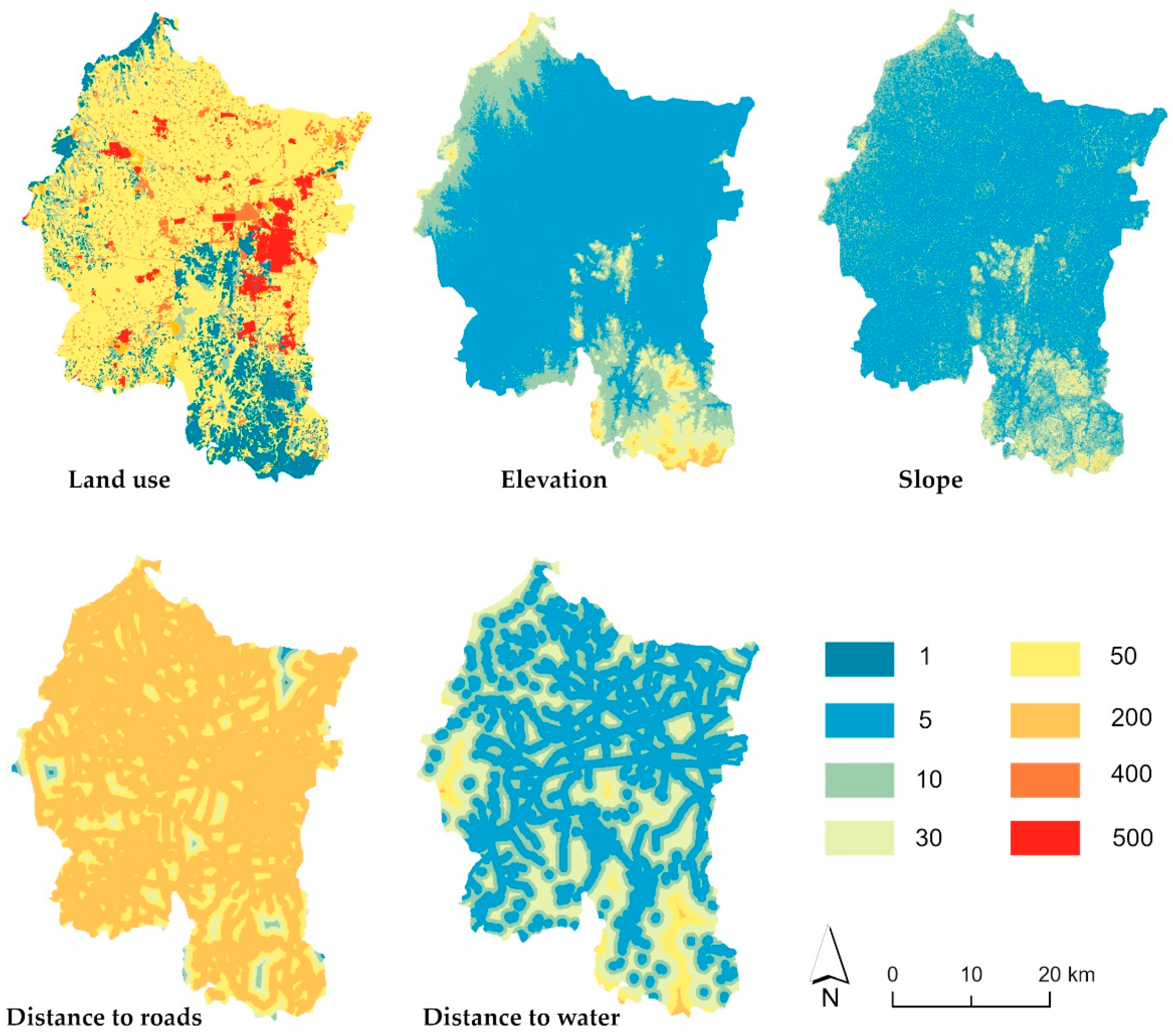
2.2. Data Sources and Processing

The basic data with different sources and precision were georeferenced in Albers Conical Equal Area projection in ArcGIS, including remote-sensing images, DEM, meteorological data, soil data, and vector data, as shown in

Table 1. Basic data.

Type	Year	Data Source	Precision	Usage
Remote sensing images	2021	USGS Landsat8 OLT_TIRS	30 m	Identification of land-use types and ecological source; resistance-surface construction
DEM	2019	Geospatial Data Cloud ASTER GDEMV3	30 m	Evaluation of ecosystem services and ecological resistance
Meteorological data	2020	China Meteorological Data Service Centre	30 m	Water-yield calculation; evaluation of soil-conservation service
Soil data	2009	FAO	30″	Evaluation of soil-conservation service
	2017	European Soil Data Center	30″
Vector data (water system, transportation, etc.)	2020	OpenStreetMap		Water-yield calculation; evaluation of soil-conservation service

. The data processing mainly consisted of the following: (1) The remote-sensing images were interpreted by ENVI5.3 to obtain six types of land use with a precision of 30 m: cultivated land, forest land, grassland, water area, construction land, and unused land; (2) the grid data of annual rainfall and evapotranspiration were obtained by spatial interpolation with ArcGIS10.6; (3) ecosystem services were evaluated by InVEST3.10 and ArcGIS10.6; (4) the connectivity importance of patches was calculated by Conefor2.6; (5) the calculation of elevation, slope, and topographic index and a comprehensive evaluation of resistance surface were carried out by ArcGIS10.6; and (6) based on the ArcGIS platform, the Linkage Mapper3.0 toolbox was used to identify ecological corridors and nodes.

2.3. Methods

The technical route is as shown in Figure 3, determined by the research framework of “ecological source identification–resistance-surface construction–ecological corridor and node extraction–ESP optimization.” It consists of four steps: (1) identifying ecological sources by the evaluation of ecosystem services and the importance of ecological patches; (2) constructing an ecological-resistance surface through the comprehensive evaluation of land use, elevation, slope, etc.; (3) extracting ecological corridors and nodes based on circuit theory; and (4) putting forward the optimization strategies for the current ESP and evaluating the optimized result in terms of network structure and landscape connectivity.

2.3.1. Granularity-Reverse Method

The granularity-reverse method is based on the idea of proof by contradiction in mathematics. First, it is assumed that there are different landscape-component structures under different granularity levels. Then, a series of landscape-pattern indexes is measured to reflect the structural characteristics at each granularity level. Finally, principal component analysis is carried out and the comprehensive scores of these landscape-component structures are calculated. The corresponding granularity with the highest score in a steady state is the optimal granularity [34,41]. In this paper, forest land, grassland, and water were taken as ecological land, and 20 raster images of ecological land at different granularities from 50 m to 1200 m were generated with ArcGIS (Figure 4). From the perspective of landscape wholeness and connectivity, 11 indexes were selected and calculated with FRAGSTATS (

Table A1. Formulas and explanations of landscape-pattern indexes [68,69].

Landscape Pattern Indexes		Acronym	Formula	Explanation
Composition	Number of patches	NP	$NP=n$	The total number of patches in the landscape
	Patch density	PD	$PD=\frac{n}{A}\left(10,000\right)\left(100\right)$	The number of patches within 100 hectares
	Largest patch index	LPI	$LPI=\frac{\max {\left(a_{ij}\right)}_{j=1}^n}{A}$ where $a_{ij}$ is the area of patch $ij$, A is the total landscape area	The percentage of the landscape comprised by the largest patch
Shape	Landscape shape index	LSI	$LSI=\frac{0.25{{\displaystyle \sum }}_{k=1}^m{e}_{ik}^{*}}{\sqrt{A}}$ where $e_{ik}^{*}$ is the total length of edges in landscape between patch types $i$ and $k$, A is the total landscape area	This index provides a standardized measure of total edge or edge density that adjusts for the size of the landscape.
Aggregation	Mean proximity index	PROX_MN	$PROX\_MN=\frac{{{\displaystyle \sum }}_{j=1}^n{{\displaystyle \sum }}_{s=1}^n\frac{a_{ijs}}{h_{ijs}^2}}{n_i}$ where, $a_{ijs}$ is the area of patch $ijs$ within a specified neighborhood of patch $ij$, $h_{ijs}$ is the distance between patch $ijs$ and patch $ij$, $n$ is the total number of patches	This index considers the size and proximity of all patches whose edges are within a specified search radius of the focal patch. It increases as patches become less isolated and the patch type becomes less fragmented in distribution.
	Proportion of like adjacencies	PLADJ	$PLADJ=\left(\frac{g_{ii}}{{{\displaystyle \sum }}_{k=1}^m{g}_{ik}}\right)\left(100\right)$ where $g_{ii}$ is the number of like adjacencies between pixels of patch type $i$, $g_{ik}$ is the number of adjacencies between pixels of patch types $i$ and $k$.	This index is calculated from the adjacency matrix, which shows the frequency with which different pairs of patch types appear side-by-side on the map. It measures the degree of aggregation of the focal-patch type.
	Connectance index	CONNECT	$CONNECT=\left(\frac{{{\displaystyle \sum }}_{j=k}^n{c}_{ijk}}{\frac{n_i\left(n_i-1\right)}{2}}\right)\left(100\right)$ where $c_{ijk}$ is the joining between patch $j \mathrm{and} k, n_i$ is the number of patches of the corresponding patch type	This index is reported as a percentage of the maximum possible connectance given the number of patches.
	Patch-cohesion index	COHESION	$COHESION=\left[1-\frac{{{\displaystyle \sum }}_{j=1}^n{p}_{ij}^{*}}{{{\displaystyle \sum }}_{j=1}^n{p}_{ij}^{*}\sqrt{a_{ij}^{*}}}\right]·{\left[1-\frac{1}{\sqrt{Z}}\right]}^{-1}·\left(100\right)$ where $p_{ij}^{*}$ is the perimeter of patch $ij$ in terms of number of cell surfaces, $a_{ij}^{*}$ is the area of patch $ij$ in terms of number of cells, $Z$ is the total number of cells in the landscape	This index measures the physical connectedness of the corresponding patch type. It increases as the patch type becomes more clumped or aggregated in its distribution.
	Landscape-division index	DIVISION	$DIVISION=\left[1-{\displaystyle \sum }_{i=1}^m{\displaystyle \sum }_{j=1}^n{\left(\frac{a_{ij}}{A}\right)}^2\right]$ where $a_{ij}$ is the area of patch $ij$, $A$ is the total landscape area	This index is interpreted as the probability that two randomly chosen pixels in the landscape are not situated in the same patch.
	Splitting index	SPLIT	$SPLIT=\frac{A^2}{{{\displaystyle \sum }}_{i=1}^m{{\displaystyle \sum }}_{j=1}^n{a}_{ij}^2}$ where $a_{ij}$ is the area of patch $ij$, $A$ is the total landscape area	This index is interpreted as the effective mesh number and increases as the focal-patch type is increasingly reduced in area and subdivided into smaller patches.
	Aggregation index	AI	$AI=\left[\frac{g_{ii}}{max-g_{ii}}\right]\left(100\right)$ where $g_{ii}$ is the number of like adjacencies between pixels of patch type $i$, $max-g_{ii}$ is the maximum number of like adjacencies between pixels of patch type $i$	This index shows the frequency with which different pairs of patch types appear side-by-side on the map. It increases as the focal-patch type is increasingly aggregated.

). NP (number of patches), PD (patch density), and LPI (largest patch index) are the indexes describing the landscape-composition status. LSI (landscape-shape index) is the index indicating the edge complexity of the landscape shape. The indexes analyzing the degree of landscape aggregation are PROX_MN (mean-proximity index), PLADJ (proportion of like adjacencies), CONNECT (connectance index), COHESION (patch-cohesion index), DIVISION (landscape-division index), SPLIT (splitting index), and AI (aggregation index).

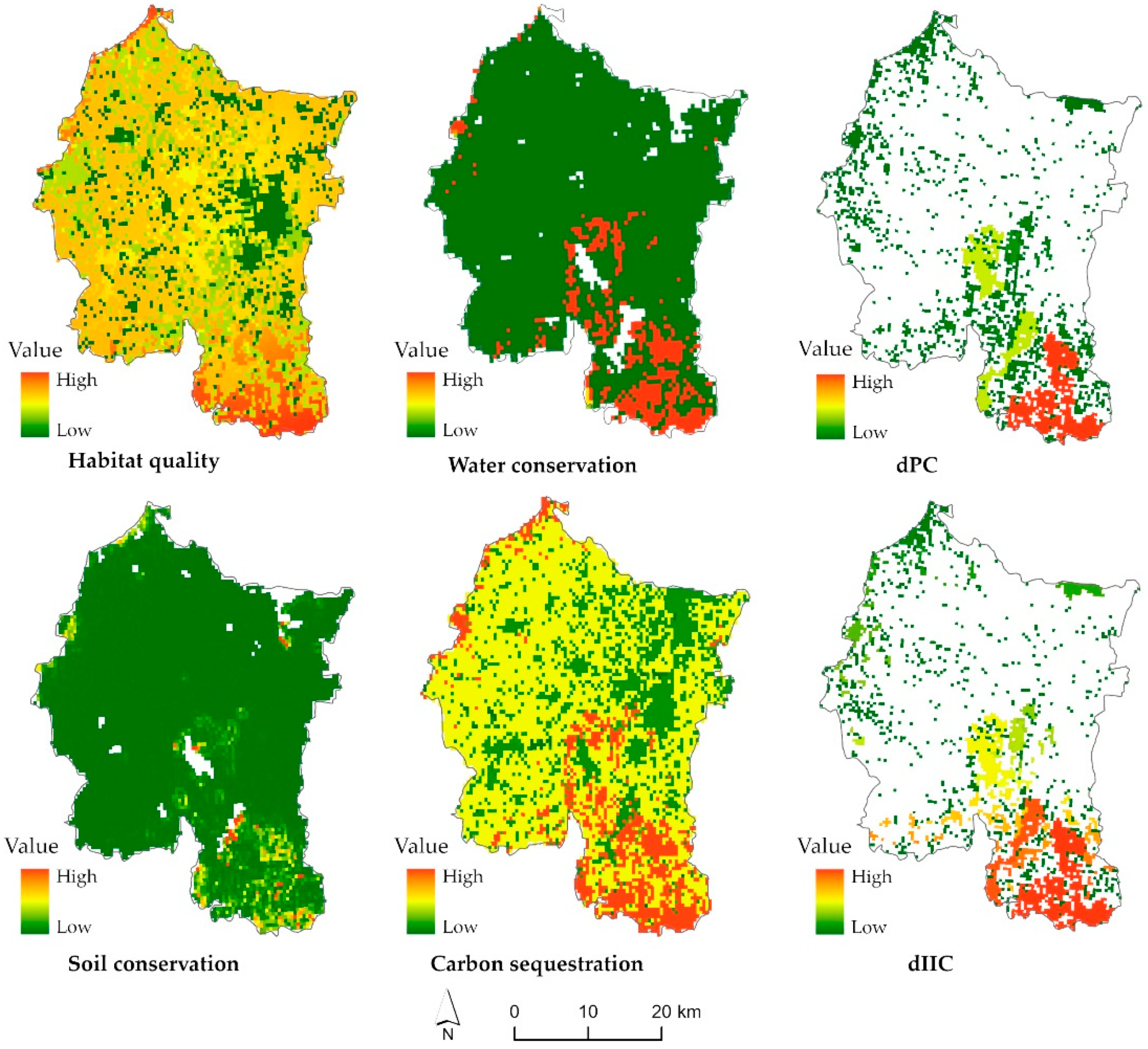
2.3.2. Ecosystem-Service Evaluation

Ecosystem services cover a wide range of benefits obtained directly or indirectly by humans and are key indicators for measuring ecosystem health [42]. Ecological sources not only provide habitats for native species but also provide important ecosystem services for humans [43]. Habitat quality is an essential index to be considered, since it is closely related to the biological growth, foraging, and reproduction of wildlife. Given that frequent rainstorms in recent years can increase the risk of soil erosion in topographic-relief areas of Liyang City, soil conservation is also an important factor to be considered. Since there are large-scale lakes and dense river networks in this region, water conservation is another key ecosystem service. Terrestrial ecosystems, such as forests, grasslands, and wetlands, can absorb CO₂ and regulate the local climate, so carbon sequestration likewise merits attention. With a comprehensive consideration of the city’s ecological characteristics, the demand for ecosystem services, and data availability, four ecological services of habitat quality, soil conservation, water conservation, and carbon sequestration were selected and calculated with the help of the InVEST model. The integrated ecosystem-service function was evaluated by normalization and superposition analysis. The specific evaluation methods and calculation processes are shown in

Table 2. Methods and calculation processes for ecosystem-service evaluation.

Index	Method	Calculation Formula	Explanation
Habitat quality	InVEST Habitat Quality Model	$Q_{xj}$$=H_j$$[1-(\frac{D_{xj}^z}{k^z+D_{xj}^{\mathrm{z}}}\left)\right]$	$Q_{xj}$ is the habitat quality of raster $x$ in land-use type $j$; $H_j$ is the habitat suitability of land-use type $j$ $D_{xj}$ is the degree of habitat degradation of grid $x$ in land-use type $j$; $k$ is a half-saturation constant, typically assigned a value of 0.5; $z$ is a scaling parameter and is 2.5 in this paper.
Soil conservation	InVEST SDR(Seddiment Delivery Ratio) Model	$SEDRE{T}_x=R_x\times K_x\times L{S}_x\times \left(1-C_x\times P_x\right)+SED{R}_x$	$SEDRE{T}_x$ is the amount of soil conservation; $SED{R}_x$ is the amount of sediment retention; $R_x$, $K_x$ and $L{S}_x$ are rainfall erosivity, soil erodibility, and slope length-gradient factor in grid $x$, respectively; $C_x$ and $P_x$ are a cover-management factor and a support practice factor in grid $x$, respectively.
Water conservation	Obtain water yield by InVEST Annual Water Yield Model and complete the calculation with the listed formula	$R=min\left(1,\frac{249}{velocity}\right)\times min\left(1,\frac{0.9\times TI}{3}\right)\times min\left(1,\frac{Ks}{300}\right)\times Y_x$	$R$ is the amount of water conservation; $velocity$ is the velocity coefficient; $TI$ is the topographic index; $K_s$ is the saturated hydraulic conductivity; $Y_x$ is the water yield in grid $x$.
Carbon sequestration	InVEST Carbon Storage and Sequestration Model	$C_i=C_{i-above}+C_{i-below}+C_{i-soil}$ $C_{total}={\displaystyle \sum }_{i=1}^n{C}_i\times S_i$	The amount of carbon stored and sequestered is estimated according to land-use types from aboveground biomass, belowground biomass, and soil. In the formula $i$ refers to a certain land-use type, including n types; $C_i$ means the carbon density of land use $i$; $C_{i-above}$, $C_{i-below}$ and $C_{i-soil}$ are the aboveground carbon density, belowground carbon density, and soil carbon density of land use $i$, respectively; $C_{total}$ is the total amount of carbon storage; $S_i$ is the area of land use $i.$

[42,43,44,45,46,47,48,49,50].

2.3.3. Connectivity Evaluation

Landscape connectivity is a measure of the continuity among landscape spatial-structure units [30], reflecting the extent to which landscape promotes or hinders species movement among the patches [51,52]. Higher landscape connectivity is conducive to maintaining ecological processes and biodiversity. In this study, connectivity was analyzed with Conefor2.6, which is a simple program for quantifying landscape connectivity and the importance of habitat patches for maintaining landscape connectivity through combining graphical structures and habitat-availability indexes [53]. The distance threshold was set to 1000 m and the probability of connectivity to 0.5 [54,55].

The probability of connectivity (PC) and the integral index of connectivity (IIC) were selected for the evaluation of landscape-level connectivity, which can be used to judge the effect of the optimized ESP in the study area. The calculation formulas are as follows:

$$PC=\frac{{{\displaystyle \sum }}_{i=1}^n{{\displaystyle \sum }}_{j=1}^n{a}_{i·}{a}_j·P_{ij}^{*}}{A_L^2}$$

(1)

$$IIC=\frac{{{\displaystyle \sum }}_{i=1}^n{{\displaystyle \sum }}_{j=1}^n\left(\frac{a_{i·}{a}_j}{1+n{l}_{ij}}\right)}{A_L^2}$$

(2)

where n is the total number of patches in the study area; $a_i$ and $a_j$ represent the areas of patch $i$ and patch $j$, respectively, which presents the maximum probability of species spreading between patch $i$ and patch $j$, respectively; $n{l}_{ij}$ is the number of links in the shortest path (topological distance) between patches $i$ and $j$; and $A_L$ is the total area of the landscape.

The $dPC$ and $dIIC$ indexes were selected to calculate the connectivity importance of patches. The principle is that the change in landscape connectivity after removing a patch reflects the importance of the patch. The larger the value, the greater the difference between before and after the patch is removed—that is, the more important the patch is. For ecological-source identification, the importance of patches is also a factor to be considered, and the calculation formulas are as follows:

$$dPC=\frac{PC-P{C}_{remove}}{PC}\times 100\%$$

(3)

$$dIIC=\frac{dIIC-dII{C}_{remove}}{dIIC}\times 100\%$$

(4)

where $dPC$ and $dIIC$ represent the patch importance for maintaining the overall probability of connectivity ($PC$) and integral index of connectivity ($IIC$), respectively; $P{C}_{remove}$ is the value of $PC$ after removing a specific patch; and $II{C}_{reomve}$ is the value of $IIC$ after removing a specific patch.

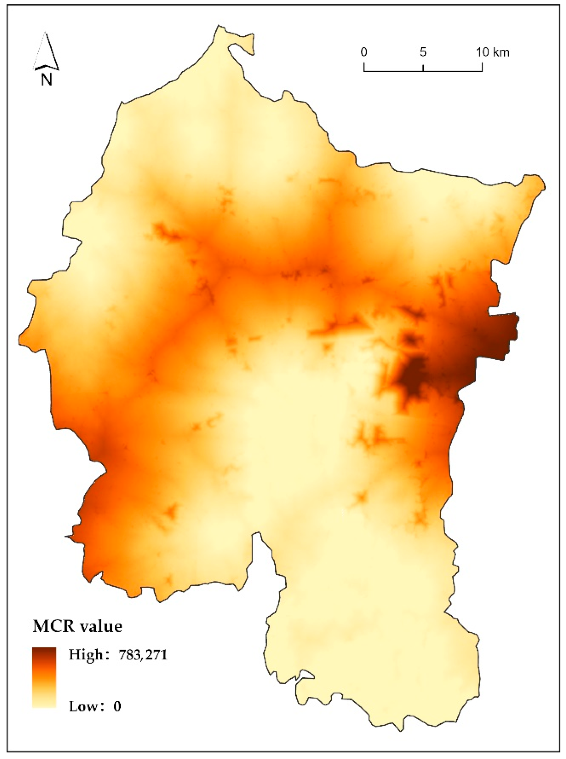
2.3.4. Construction of Ecological-Resistance Surface

Ecological resistance refers to the degree to which species are facilitated or impeded when they are dispersed over different landscape patches [56]. The higher the value, the more difficult spatial migration and circulation will be. The ecological-resistance surface shows the spatial distribution of the regional ecological resistance and is constructed by comprehensive evaluation [57]. With reference to relevant studies [1,29,35,58,59], the natural conditions (land-use type, elevation, and slope) and human-activity factors (distance from roads and distance from waterbodies) are comprehensively considered, and five indexes were accordingly identified, as shown in

Table 3. Resistance-factor assignment table.

Indexes	Weight	Factors	Resistance Value
Land-use type	0.5	Cultivated land	50
		Forest land	1
		Water area	50
		Grassland	10
		Urban and other construction land	500
		Rural residential area	400
		Unused land	200
Elevation (m)	0.15	<29	5
		29–72	10
		72–141	30
		141–246	50
		246–509	200
Slope (°)	0.1	0–5	5
		5–15	10
		15–25	30
		25–35	50
		>35	200
Distance from roads (km)	0.1	<0.5	200
		0.5–1	100
		1–2	30
		2–3	10
		>3	5
Distance from waterbodies (km)	0.15	<1	5
		1–3	10
		3–5	30
		5–8	50
		>8	200

. The resistance values ranged from 1 to 500. The weight of each index was determined with a hierarchical-analysis process [60].

2.3.5. Extraction of Ecological Corridors and Nodes

Ecological corridors and ecological nodes are important components of ESP. Ecological corridors are low-cumulative-resistance areas among ecological sources. They are important channels for material cycling and energy flow, and are major pathways for species migration [33]. Ecological nodes are the stepping stones in the corridor network with strategic significance for the connectivity and stability of ESP, and need to be protected and restored. In this study, the minimum-cumulative-resistance (MCR) model and circuit theory were applied to extract ecological corridors and nodes. The MCR model can simulate the resistance that needs to be overcome in the process of species migration, and the paths with the lowest cumulative resistance are the ecological corridors among the patches. The calculation formula is as follows [23,61]:

$$MCR=f_{min}{\displaystyle \sum }_{J=0}^{i=m}\left(Dij\times R_i\right)$$

(5)

where $MCR$ is the minimum-cumulative-resistance value, $f$ represents the positive-correlation function between the MCR and the ecological process, $D_{ij}$ is the spatial distance of species from the ecological source $j$ to the landscape unit $i$, and $R_i$ is the resistance value of the landscape unit $i$ to the movement of species.

The extraction of ecological corridors was performed with the Build Network and Map Linkages tools in the Linkage Mapper 3.0 toolbox. In circuit theory, ecological sources are equivalent to circuit nodes, and the non-ecological-source areas are equated with the resistors with different resistance values. The random walk of electrons in the circuit was used to simulate the migration process of individual species in the landscape so as to predict the movement law of species and identify multiple paths in the landscape surface—that is, the ecological corridors [30,51]. Ecological nodes include barrier points and pinch points, which could be identified by the Barrier Mapper and Pinchpoint Mapper tools in the Linkage Mapper 3.0 toolbox.

2.3.6. Network-Structure Assessment

The network-analysis method based on graph theory can effectively evaluate the connectivity and complexity of the structure of an ecological network [62]. The alpha index (α), beta index (β), and gamma index (γ) were selected as the evaluation indexes. The alpha index with a value range from 0 to 1 reflects the degree of circuitry, and the greater the value the smoother the circulation in the network [63]. The beta index shows the average number of connections per node in the network, which can reflect the complexity of network connections and takes a value between 0 and 3 [64]. When β ≤ 1, it means that the network structure is simpler, and β > 1 means that the network structure is more complex. The gamma index is the ratio of the number of corridors to the maximum possible number of corridors, which is used to describe the degree of connectivity of all nodes to the network [63]. The value range is between 0 and 1, and the larger the value the higher the degree of connectivity. The calculation formulas are as follows [40,65]:

$$\alpha =\frac{L-V+1}{2V-5}$$

(6)

$$\beta =\frac{\mathrm{L}}{V}$$

(7)

$$\gamma =\frac{L}{3\left(V-2\right)}$$

(8)

where $V$ is the number of nodes, and $L$ is the number of corridors.

3. Results

3.1. Ecological Sources

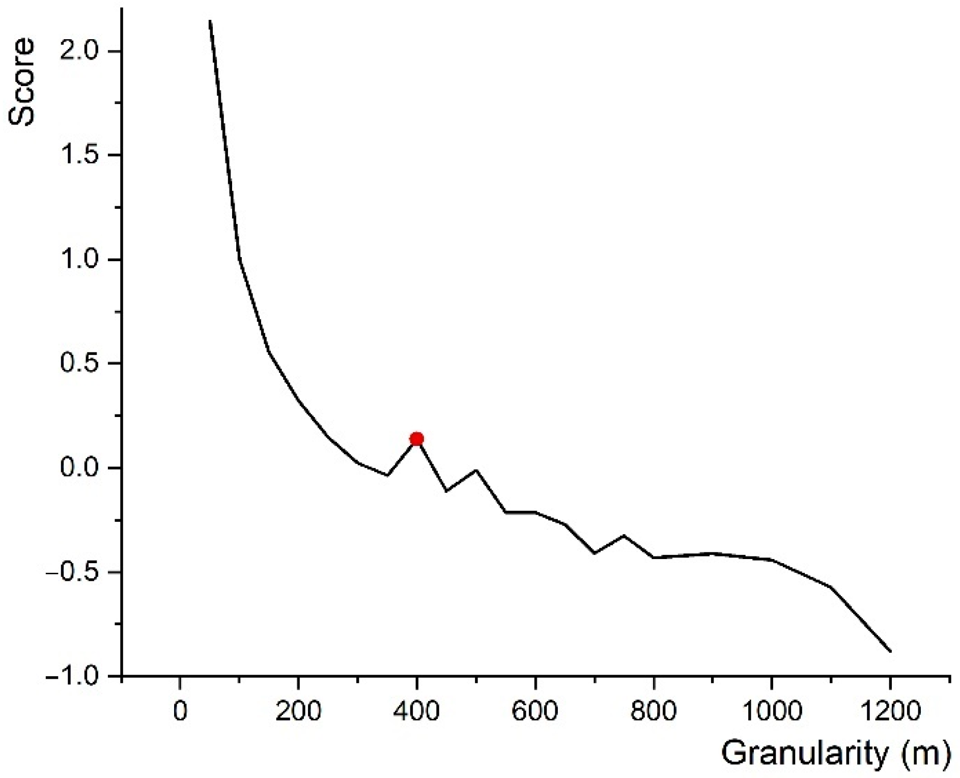
3.1.1. Optimal-Granularity Determination

The 11 landscape-pattern indexes at 20 granularities were calculated with FRAGSTATS, and the results are show in Table 4. The KMO and Bartlett’s test of sphericity showed that the KMO was 0.746, which is greater than 0.7, and the sig. value was less than 0.05, indicating that the data support the principal component analysis (Table 5). With the criteria of eigenvalues greater than 1 and a cumulative-variance contribution greater than 90%, three factors were extracted (Table 6 and Table 7). Factor 1 was closely related to NP, PD, LSI, PROX_MN, PLADJ, COHESION, and AI, which reflect the agglomeration of landscape structure and can be considered the wholeness indexes. In factor 2, LPI, DIVISION, and SPLIT were more closely related and could be categorized as fragmentation indexes, showing the discrete degree of landscape components. Factor 3 had a higher correlation with CONNECT, which is the connectivity index. The weights of the principal components were calculated by the variable loads and eigenvalues, and the functional expressions of each principal component score are as follows:

Z₁ = 0.371zX₁ + 0.371zX₂ − 0.076zX₃ + 0.381zX₄ + 0.372zX₅ + 0.381zX₆ + 0.35zX₈ + 0.071zX₉ + 0.134zX₁₀ + 0.38zX₁₁

(9)

Z₂ = 0.176zX₁ + 0.176zX₂ − 0.542zX₃ + 0.155zX₄ + 0.142zX₅ + 0.144zX₆ − 0.031zX₇ − 0.116zX₈ + 0.532zX₉ + 0.509zX₁₀ + 0.15zX₁₁

(10)

Z₃ = −0.055zX₁ − 0.053zX₂ + 0.052zX₃ − 0.004zX₄ − 0.069zX₅ − 0.002zX₆ + 0.946zX₇ + 0.288zX₈ − 0.089zX₉ + 0.027zX₁₀ − 0.019zX₁₁

(11)

According to the variance-contribution rate of each factor, the calculation formula of the composite score was derived as follows:

Z = 0.575 Z₁ + 0.3Z₂ + 0.1Z₃

(12)

where Z is the composite score; Z₁, Z₂, and Z₃ are the scores of the three factors; and zX₁ − zX₁₁ corresponds to the standardized values of each index in Table 4.

Table 4. Statistics of landscape-pattern index measurement.

Granularity (m)	NP X1	PD X2	LPI X3	LSI X4	PROX_MN X5	PLADJ X6	CONNECT (%) X7	COHESION (%) X8	DIVISION X9	SPLIT X10	AI(%) X11
50	2400	6.73	20.51	60.76	291.63	83.90	1.86	98.06	0.91	11.15	84.13
100	1828	5.12	54.38	48.15	280.23	74.52	1.61	98.08	0.70	3.34	74.91
150	1251	3.51	55.79	39.26	154.64	68.75	1.58	97.59	0.69	3.18	69.30
200	865	2.43	54.33	33.10	94.41	64.93	1.58	96.85	0.70	3.34	65.62
250	635	1.77	56.12	28.97	67.85	61.67	1.66	96.48	0.68	3.13	62.49
300	474	1.34	55.32	25.44	54.35	59.26	1.62	95.83	0.69	3.22	60.23
350	363	1.02	56.26	22.50	41.17	58.22	1.73	95.52	0.68	3.11	59.32
400	257	0.73	40.32	20.13	22.28	56.74	1.81	93.69	0.80	5.11	57.99
450	252	0.72	52.81	19.07	26.88	53.57	1.84	93.89	0.71	3.50	54.90
500	195	0.54	42.26	17.50	14.10	53.85	1.80	92.77	0.79	4.74	55.31
550	171	0.47	57.89	16.16	19.66	52.56	1.94	94.44	0.66	2.94	54.15
600	144	0.39	56.80	15.00	15.27	52.66	1.98	93.62	0.67	3.04	54.38
650	135	0.38	55.15	14.54	14.85	49.23	1.96	92.91	0.69	3.22	51.01
700	102	0.29	59.07	13.07	10.86	50.00	1.75	93.53	0.64	2.80	51.99
750	95	0.27	60.48	12.38	11.22	50.48	2.06	93.33	0.63	2.68	52.58
800	96	0.26	60.95	12.27	7.92	48.42	1.91	93.03	0.62	2.66	50.55
900	79	0.22	43.51	11.10	4.35	46.92	1.59	87.84	0.78	4.57	49.28
1000	62	0.18	58.77	10.41	5.50	43.71	2.22	90.63	0.64	2.82	46.21
1100	60	0.16	39.35	9.36	2.58	45.65	1.19	85.57	0.81	5.24	48.46
1200	49	0.13	59.62	8.48	2.65	46.15	1.02	89.53	0.64	2.75	49.28

Table 4. Statistics of landscape-pattern index measurement.

Granularity (m)	NP X1	PD X2	LPI X3	LSI X4	PROX_MN X5	PLADJ X6	CONNECT (%) X7	COHESION (%) X8	DIVISION X9	SPLIT X10	AI(%) X11
50	2400	6.73	20.51	60.76	291.63	83.90	1.86	98.06	0.91	11.15	84.13
100	1828	5.12	54.38	48.15	280.23	74.52	1.61	98.08	0.70	3.34	74.91
150	1251	3.51	55.79	39.26	154.64	68.75	1.58	97.59	0.69	3.18	69.30
200	865	2.43	54.33	33.10	94.41	64.93	1.58	96.85	0.70	3.34	65.62
250	635	1.77	56.12	28.97	67.85	61.67	1.66	96.48	0.68	3.13	62.49
300	474	1.34	55.32	25.44	54.35	59.26	1.62	95.83	0.69	3.22	60.23
350	363	1.02	56.26	22.50	41.17	58.22	1.73	95.52	0.68	3.11	59.32
400	257	0.73	40.32	20.13	22.28	56.74	1.81	93.69	0.80	5.11	57.99
450	252	0.72	52.81	19.07	26.88	53.57	1.84	93.89	0.71	3.50	54.90
500	195	0.54	42.26	17.50	14.10	53.85	1.80	92.77	0.79	4.74	55.31
550	171	0.47	57.89	16.16	19.66	52.56	1.94	94.44	0.66	2.94	54.15
600	144	0.39	56.80	15.00	15.27	52.66	1.98	93.62	0.67	3.04	54.38
650	135	0.38	55.15	14.54	14.85	49.23	1.96	92.91	0.69	3.22	51.01
700	102	0.29	59.07	13.07	10.86	50.00	1.75	93.53	0.64	2.80	51.99
750	95	0.27	60.48	12.38	11.22	50.48	2.06	93.33	0.63	2.68	52.58
800	96	0.26	60.95	12.27	7.92	48.42	1.91	93.03	0.62	2.66	50.55
900	79	0.22	43.51	11.10	4.35	46.92	1.59	87.84	0.78	4.57	49.28
1000	62	0.18	58.77	10.41	5.50	43.71	2.22	90.63	0.64	2.82	46.21
1100	60	0.16	39.35	9.36	2.58	45.65	1.19	85.57	0.81	5.24	48.46
1200	49	0.13	59.62	8.48	2.65	46.15	1.02	89.53	0.64	2.75	49.28

Table 5. KMO and Bartlett’s test.

Kaiser–Meyer–Olkin Measure of Sampling Adequacy		0.746
Bartlett’s Test of Sphericity	Approx. Chi-Square	708.871
	df	55
	Sig.	0.000

Table 5. KMO and Bartlett’s test.

Kaiser–Meyer–Olkin Measure of Sampling Adequacy		0.746
Bartlett’s Test of Sphericity	Approx. Chi-Square	708.871
	df	55
	Sig.	0.000

Table 6. Statistics of variance-contribution rate.

Component	Eigenvalue	Variance Contribution Rate (%)	Accumulative Contribution Rate (%)
1	6.329	57.533	57.533
2	3.249	29.539	87.073
3	1.101	10.006	97.078
4	0.230	2.092	99.170
5	0.075	0.678	99.849
6	0.008	0.075	99.924
7	0.007	0.062	99.986
8	0.001	0.010	99.996
9	0.000	0.004	100.000
10	1.240 × 10−5	0.000	100.000
11	6.217 × 10−6	5.651 × 10−5	100.000

Table 6. Statistics of variance-contribution rate.

Component	Eigenvalue	Variance Contribution Rate (%)	Accumulative Contribution Rate (%)
1	6.329	57.533	57.533
2	3.249	29.539	87.073
3	1.101	10.006	97.078
4	0.230	2.092	99.170
5	0.075	0.678	99.849
6	0.008	0.075	99.924
7	0.007	0.062	99.986
8	0.001	0.010	99.996
9	0.000	0.004	100.000
10	1.240 × 10−5	0.000	100.000
11	6.217 × 10−6	5.651 × 10−5	100.000

Table 7. Component matrix.

Variables	Factors
	F1	F2	F3
NP	0.934	0.318	−0.057
PD	0.935	0.318	−0.056
LPI	−0.192	−0.978	0.054
LSI	0.958	0.280	−0.004
PROX_MN	0.935	0.256	−0.073
PLADJ	0.958	0.259	−0.002
CONNECT	0.000	−0.055	0.992
COHESION	0.880	−0.209	0.302
DIVISION	0.179	0.958	−0.093
SPLIT	0.336	0.918	0.028
AI	0.957	0.271	−0.020

Table 7. Component matrix.

Variables	Factors
	F1	F2	F3
NP	0.934	0.318	−0.057
PD	0.935	0.318	−0.056
LPI	−0.192	−0.978	0.054
LSI	0.958	0.280	−0.004
PROX_MN	0.935	0.256	−0.073
PLADJ	0.958	0.259	−0.002
CONNECT	0.000	−0.055	0.992
COHESION	0.880	−0.209	0.302
DIVISION	0.179	0.958	−0.093
SPLIT	0.336	0.918	0.028
AI	0.957	0.271	−0.020

The composite scores of landscape-composition structure at each granularity are shown in Figure 5. With the increase in granularities, small and isolated patches were continuously eliminated, the number of patches was reduced, adjacent patches were continuously merged, and landscape components were gradually dispersed. Therefore, the trend of composite scores presented an overall decline with local fluctuation. The score peaked at the granularity of 400 m and was significantly higher than that of both sides, indicating that the landscape composition reached a suitable structure at this threshold. Thus, the granularity of 400 m was a critical point that provided a suitable research scale for identifying ecological sources.

3.1.2. Identification of Ecological Sources

As shown in Figure 6, the ecosystem services (habitat quality, water conservation, soil conservation, and carbon sequestration) and the connectivity importance of ecological patches (dPC and dIIC) were quantitively evaluated at a granularity of 400 m. In terms of the evaluation of ecosystem services, the southern part of the study area performed best, as large ecological patches such as Daxi Reservoir, Tianmu Lake, and Nanshan Bamboo Sea provided rich ecological benefits for the city. At the northern boundary, there are also large ecological patches, such as Cao Mountain, Wawu Mountain, and Changdang Lake, that provided good ecosystem services. In comparison, the ecosystem services in the west and east of the study area were poor. As to the patch importance evaluation, it was also the southern part of the city that performed well. The comprehensive evaluation was made by superposing the results above. Finally, 24 patches with high scores and larger than 1 km² were selected as ecological sources, with a total area of 162.9 km² (Figure 7).

3.2. Ecological-Resistance Surface

The five factors of land-use type, elevation, slope, distance from traffic, and distance from water were evaluated according to Table 3 and as shown in Figure 8. The comprehensive-resistance surface was created by the superposition of every single factor with the corresponding weights, as shown in Figure 9. The minimum-cumulative-resistance (MCR) surface was obtained by the Cost Distance tool of ArcGIS, as shown in Figure 10. The MCR value was low in ecological sources and their peripheries and gradually increased with the incremental distance from the ecological sources. High-value areas were located in the north–central part of the city, as well as in the east and west. The maximum value was observed around the central city on the east side.

3.3. Ecological-Security Pattern

By grading the minimum-cumulative-resistance surface with a natural break, the ecological-security level was divided into high, medium, and low levels in the study area. Combined with the spatial distribution of ecological sources, the ESP zones were categorized as “core protected zone,” “general protected zone,” “coordinated-control zone,” and “restoration-improvement zone” (Figure 11a). The core protected zone is where the ecological sources are distributed, accounting for 10.6% of the total area. This zone is the core area to maintain the ecological balance, with high ecosystem services and high ecological sensitivity. The general protected zone is the area with a high level of ecological security surrounding the core protection zone, accounting for 21.66% of the total area. This zone is the security screen of ecological sources and a favorable space for species dispersal, but still has fragile ecological conditions in some parts and needs timely monitoring and protection. The coordination-control zone is the medium-level ecological-security area, accounting for 28.27% of the total area. It is a transitional zone for coordinating ecological protection and human construction. Thus, the construction behavior that greatly disturbs the natural environment should be controlled in this zone, and development activities that do not harm the ecological environment such as fruit-and-vegetable planting or eco-tourism gardens should be allowed. The restoration-improvement zone is where there is a low level of ecological security, accounting for 39.47% of the total area. This zone is far from ecological sources, mainly including the built-up area of the central city, industrial and mining land, and agricultural land. It is a concentrated area for human production, living, and social and economic activities, and the ecological land here presents a fragmented spatial distribution and needs ecological-restoration improvement.

Based on the established ecological sources and resistance surface, the ecological corridors and nodes were extracted with the Linkage Mapper toolbox, and the spatial distribution of the ESP components was as shown in Figure 11b. The ecological corridors help achieve material and energy flow and species migration by communicating the ecological sources. In total, 41 corridors were obtained with a total length of 202.76 km. Centrality is an indicator measuring the importance of links for maintaining the connectivity throughout the network [66], and was calculated with the Centrality Mapper tool (Figure 12a). The Linkage Priority tool was used for calculating the priority of links. As shown in Figure 12b, the basic priority was calculated based on many factors, such as the shape and size of ecological sources, the permeability and proximity of links, and expert opinions. The blended priority was calculated by combining the linkage priority with the truncated current cost in an evenly weighted sum (Figure 12c). From the corridor analyses, it can be seen that corridors 1 and 2 had high centrality but the lowest linkage priority and a low level of blended priority. Corridor 3 had high centrality but low link priority, and the blended priority, especially in the northern section, was also at a low level. Corridor 4 had low link priority and the southern section was too narrow. Therefore, these four corridors need to be emphatically improved. Considering the electric-current intensity, corridor length, spatial location, and other factors, the ecological corridors were divided into key corridors, important corridors, and general corridors. Key corridors are scattered across the city, with a total of nine, accounting for 46% of the total length, which were the best connecting paths between ecological sources. Important corridors are the communication bridges between larger ecological sources, with a total of 12, accounting for 18% of the total length. General corridors contribute to increasing connectivity within the city, with a total of 20, accounting for 36% of the total length. A total of 50 ecological nodes were identified, including 38 ecological barrier points and 12 pinch points. Ecological barrier points refer to the areas where species are impeded during movement, and the restoration of these areas can significantly reduce ecological resistance and improve landscape connectivity [67]. The pinch points are the parts with high current density in ecological corridors, which are caused by compressing the corridors in a narrow range due to the high-value surrounding resistance. They are key areas for corridor connectivity with a high risk of ecological degradation and need to be restored and improved [43]. The analyses of ecological barriers and pinch points were carried out by the Barrier Mapper and Pinchpoint Mapper tools of the Linkage Mapper 3.0 toolbox, as shown in Figure 13. The areas with improvement scores higher than 50 were selected as ecological barriers, and the areas with the current densities greater than 0.24 were selected as pinch points. As a result, 38 ecological barrier points and 12 ecological pinch points were obtained (Figure 11b).

4. Discussion

4.1. Ecological Restoration

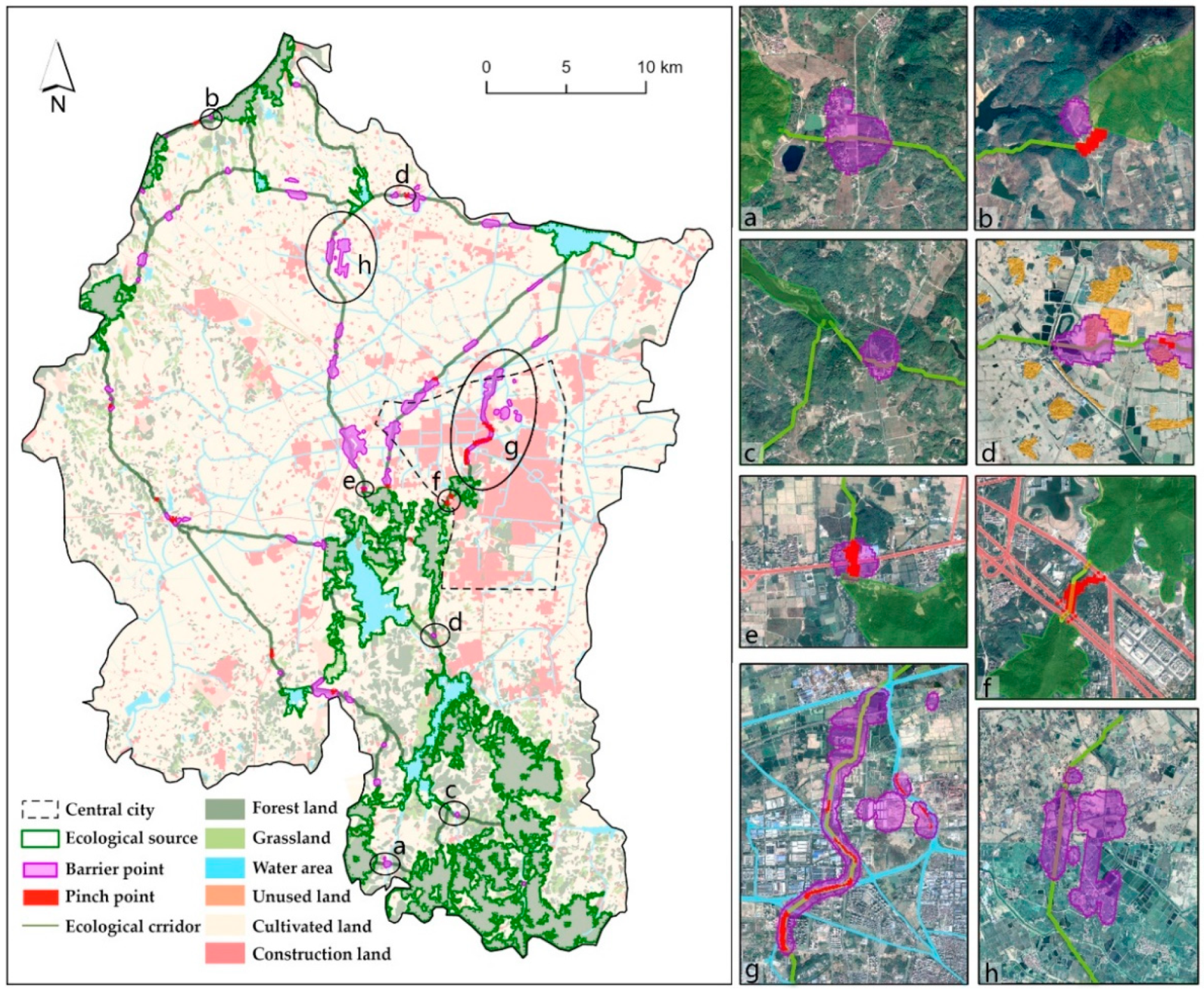
According to land-use types, ecological nodes are divided into four ecological restoration categories: farmland remediation, rural-settlement remediation, traffic optimization, and comprehensive improvement, as shown in Table 8.

The remediation of farmland needs integrated methods at the overall level. Projects such as farmland consolidation and protective forest construction should be systematically implemented to improve ecological benefits. In local areas, returning farmland to forests, grasslands and water areas can be appropriately carried out to strengthen the connectivity of ecological sources and corridors. As shown in Figure 14a,b, the embedding of farmland blocks the connection between the ecological source land and the surrounding ecological land. Thus, the farmland in the barrier area and pinch area should be transformed into woodland or grassland to extend the ecological functions from the ecological source to the corridor direction.

Rural-settlement remediation includes domestic-sewage treatment, domestic-garbage collection, and pollution control of livestock and poultry breeding. In terms of land-use adjustment, green space around the settlements should be strengthened. For example, the barrier point in Figure 14c is located in the Qingfeng Village B&B area in the south of Tianmu Lake scenic area, so first, the expansion of the B&B area should be limited and meanwhile, the surrounding woodland construction should be strengthened. Figure 14d shows a typical plain area with scattered settlements. When the corridor passes through, the barrier and pinch areas are formed due to the obstruction of the settlements, and therefore, some settlements should be merged to reserve a certain width for the ecological corridor.

Traffic optimization mainly focuses on the ecological restoration of the barrier and pinch points formed by traffic lines crossing the ecological corridors, as shown in Figure 14e,f. Since railroads and highways are important transportation facilities and cannot be directly removed, corridor-improvement facilities for species passing through should be established at the ecological breaks, such as tubular culverts, under-bridge culverts and crossroad bridges. At the same time, warning signs of wildlife crossing and slow driving should be set in the corridor buffer zones. Regular wildlife corridor monitoring should also be implemented to eliminate the interference.

The comprehensive improvement involves a variety of land-use types and faces a more complex situation that requires a combination of restoration strategies of the above three categories. As shown Figure 14h, the barrier-point area is located between the central area of Zhuze Town and Houzhou Village in Bieqiao Town, crossed by Route 1 and with 13 settlements scattered around. Thus, besides setting the slow-driving warning sign, village consolidation and land remediation should also be carried out appropriately. For the central area of the city, attention should be paid to controlling the development scale of the built-up urban area and preserving the natural attributes of the unused land. Urban green spaces such as green belts and green centers should be well developed to guarantee the continuity of the internal and external ecosystems. For example, the area shown in Figure 14g is to the northwest of the city center. The ecological barriers and pinch points are at the riverbanks and the surrounding area, involving farmland, roads, rural construction land, urban construction land, rivers, and unused land. The construction of industries and residential areas has occupied a large amount of farmland and seriously encroached on both banks of the river, leaving insufficient space for ecological corridors, so the concession and treatment of the riverbanks should be primarily considered in future planning and construction. At present, there are still some unbuilt areas along the rivers, which should be preserved as ecological green spaces to avoid large-scale development and construction.

Table 8. Ecological-restoration categories.

Categories	Numbering in Figure 11b		Land-Use Types	Restoration Methods
	Barrier Points	Pinch Points
Farmland remediation	A1–A17	1	Farmland	Returning farmland to woodland, grassland, or water area
Rural-settlement remediation	B1–B3	2, 4, 6, 12	Rural construction land	Consolidating villages or settlements and improving surrounding greenery
Traffic optimization	C1–C5	3, 5, 8–11	Road, railway	Limiting driving speed, setting warning signs, and facilitating wildlife pathways
Comprehensive improvement	D1–D4, D9		Farmland, road, rural construction land	Controlling development scale, strengthening green space construction, preserving the vacant land, restoring riverbank spaces, etc.
	D5		Farmland, road, railway, river, rural construction land
	D6, D7		Farmland, road, river, rural construction land, industrial and mining land
	D8		Farmland, road, railway, river, rural construction land, industrial and mining land
	D10		Farmland, rural construction land
	D11	7	Farmland, road, rural construction land, urban construction land, river, unused land
	D12		Urban construction land, river, unused land
	D13		Farmland, road, rural construction land, unused land

Table 8. Ecological-restoration categories.

Categories	Numbering in Figure 11b		Land-Use Types	Restoration Methods
	Barrier Points	Pinch Points
Farmland remediation	A1–A17	1	Farmland	Returning farmland to woodland, grassland, or water area
Rural-settlement remediation	B1–B3	2, 4, 6, 12	Rural construction land	Consolidating villages or settlements and improving surrounding greenery
Traffic optimization	C1–C5	3, 5, 8–11	Road, railway	Limiting driving speed, setting warning signs, and facilitating wildlife pathways
Comprehensive improvement	D1–D4, D9		Farmland, road, rural construction land	Controlling development scale, strengthening green space construction, preserving the vacant land, restoring riverbank spaces, etc.
	D5		Farmland, road, railway, river, rural construction land
	D6, D7		Farmland, road, river, rural construction land, industrial and mining land
	D8		Farmland, road, railway, river, rural construction land, industrial and mining land
	D10		Farmland, rural construction land
	D11	7	Farmland, road, rural construction land, urban construction land, river, unused land
	D12		Urban construction land, river, unused land
	D13		Farmland, road, rural construction land, unused land

Figure 14. Typical ecological-restoration areas. (a,b): typical for farmland remediation; (c,d): typical for rural-settlement remediation; (e,f): typical for traffic optimization; (g,h): typical for comprehensive improvement.

Figure 14. Typical ecological-restoration areas. (a,b): typical for farmland remediation; (c,d): typical for rural-settlement remediation; (e,f): typical for traffic optimization; (g,h): typical for comprehensive improvement.

4.2. Optimization of Ecological-Security Pattern

The optimization of an ecological-security pattern mainly focuses on the readjustment of the quantity and layout structure of the ecological land. Barrier and pinch points are the key areas for ecological-security-pattern optimization and need to be restored according to the strategies described above. Since the land readjustment requires comprehensive consideration of economic, cultural, and social equity and other factors, it is difficult to implement. Therefore, this study mainly focused on local land-use readjustment of unused and farmland in the ecological-restoration areas. A total of 12.4 km² of non-ecological land was converted into ecological land, including 5.06 km² of unused land and 7.34 km² of farmland (Figure 15b).

In terms of the ecological sources, they were concentrated in the north and south, and there were no large ecological patches in the east side, west side, or central north of the city. This is why the area was at a low level in the ecological-security zoning, and therefore, adding new ecological sources could significantly improve the ecological-security level for this region. The east part of the city is not conducive to the development of ecological sources due to the existence of the urban center and a large amount of constructed land. In the southwest, there are large-scale paddy fields, which have a significant effect on water storage, flood control, and groundwater balance. Furthermore, the surrounding rich plant community can help improve the local microclimate. Thus, the paddy fields have potential as ecological sources. Three paddy fields with better water connectivity, less traffic interference, and an area larger than 1 km² were selected as the proposed ecological sources, with new added area of 19.1 km² (Figure 15b).

The resistance values were recalculated with the adjusted land use, and the MCR surface was regenerated accordingly. Based on the adjusted MCR, a new distribution of ecological corridors was generated. As seen in Figure 15, the high-value area of MCR was reduced by 43.5 km² and the highest value was 5% lower than before. The number of ecological corridors increased from 41 to 55, and the total length of the corridors was 285.74 km, 40.9% higher than before. The nodes in the ESP network include ecological-source points and the key points. The ecological-source points were obtained by “surface-to-point” conversion of the ecological-source areas, and three new ones were added after optimization. With the hydrology tool in ArcGIS, the “valley lines” of the MCR surface were extracted, and the low-valued lines radiating outward from the sources were selected as the routes of the outward diffusion of biological flow [23]. The intersections of these radiation routes and ecological corridors are the key nodes in the ecological network, and the number was one more after optimization than before.

In order to evaluate the effectiveness of the ESP optimization, the landscape connectivity and network structure were measured.

Table 9. Evaluation indexes before and after the ESP optimization.

Indexes	Landscape Connectivity		Network Structure
	PC	IIC	α	β	γ
Before	0.026	0.013	0.169	1.281	0.456
After	0.032	0.018	0.254	1.447	0.509

shows the comparison of the indexes before and after optimization. The indexes of landscape connectivity are PC and IIC, and both increased, showing that the connections between ecological patches were improved. The indexes of network structure are the alpha index (α), beta index (β) and gamma index (γ), all of which significantly increased, indicating that the optimized ecological network structure is more complex with more ecological flow loops, which has a positive impact on regional energy flow and material circulation.

Figure 15. Network analysis of the ESP optimization. (a) ESP network before optimization; (b) ESP network after optimization.

Figure 15. Network analysis of the ESP optimization. (a) ESP network before optimization; (b) ESP network after optimization.

4.3. Methodological Advantages

In the framework of this study, ESP optimization was added after the typical research paradigm “ecological-source identification–resistance-surface construction–corridor extraction,” making an integration of guidance and practice. Thus, the new framework is more convincing and solid.

For ecological-source identification, the optimal granularity was first determined with the granularity-reverse method, and the evaluation based on it involved both ecosystem services and the connectivity importance of patches. The accuracy of ESP was improved by fully considering the scale effect, ecological status of the study area, and the patches themselves.

Based on circuit theory, the ESP components were extracted by Linkage Mapper. Detailed analyses of ecological corridors and nodes were also conducted, including LCP centrality, linkage priority, and current-flow density, as shown in Figure 12 and Figure 13. With an in-depth understanding of ESP, corridors can be classified and key areas for ecological restoration can be identified.

This study proposed ESP zoning at the overall city level and the optimization strategies at the site scale. This can be helpful to both the macroscopic management and microscopic modification of ESP. The ESPs before and after optimization were evaluated in terms of both landscape connectivity and network structure, and the validity of the optimized result was clearly verified.

4.4. Limitations and Future Research Directions

In ecological-source identification, the importance of patches was evaluated by calculating the indexes $dPC$ and $dIIC$, but this is not the only way. Another method that can be used to identify important patches is morphological spatial-pattern analysis. In MSPA, landscape patches are divided into seven types. The core and islet are blocky ecological spaces for habitats, which have the potential to be selected as ecological sources [32]. This method will be attempted in future research, and efforts will be made to identify ecological sources with more reasonability from multiple methods.

The evaluation of connectivity was made with Conefor2.6, and the distance threshold of the landscape needs to be set, with the consideration of species-diffusion distance. Since there is no unified standard for the assignment of this parameter, the distance-threshold value in this study was set to 1000 m in reference to previous studies [54,55]. Whether this value is applicable to the study site and how to determine the distance threshold need to be further explored.

ESP optimization in this paper was mainly about local land readjustment, especially for unused land and farmland, which are easy to transform. In fact, land readjustment is a comprehensive project involving multiple sectors and various social relationships. Transportation, economic, social, environmental and community factors should be considered in future research.

5. Conclusions

Since the 20th century, a series of environmental problems such as global warming, biodiversity loss, and soil loss have attracted widespread international concern. On the national-state level, most countries in the world have enacted environmental protection regulations and formulated a framework for ecological development. For developing countries like China, where the ecological land is under the threat of being encroached on by rapid human development and construction, the primary prerequisite for the harmonious coexistence between man and nature is to keep the natural ecological-security boundary. Although a wide range of research and practice on ESP construction and optimization have been carried out, there still exist deficiencies in methodology accuracy, detailed analysis, and optimization implementability. This paper takes Liyang City as an example to explore the improvement of the deficiencies. A combination methodology of circuit theory, graph theory, the granularity-reverse method, and the comprehensive-evaluation method was applied for ESP construction, and optimization strategies were proposed further, as well as an optimization assessment.

Research results of the case study show the following: (1) The optimal granularity for identifying ecological sources was 400 m, and 24 ecological sources were identified with a total area of 162.9 km². (2) According to the leveled ecological security, the study area was divided into four zones: the core protected zone, general protected zone, coordinated-control zone, and restoration-improvement zone. (3) The current ESP includes 41 ecological corridors and 50 ecological nodes that need ecological restoration. In the optimized ESP, 31.5 km² of ecological land were added, 3 eco-logical sources were added, 55 ecological corridors were generated, and the number of nodes in the ecological network was increased by 4. (4) The results of ESP optimization evaluation show that the landscape connectivity and ecological network structure were improved, indicating that the optimization scheme has a promoting effect on the ecological coordination of Liyang City and a spatial guiding effect on regional development.

There are still some issues that need to be explored in the future—for example, how to determine the distance threshold for connectivity evaluation and how to improve the accuracy of ESP construction from multiple methods. Taking into account the coupling of security pattern and ecological processes, there are still some factors that have not been fully considered, such as the spreading process of air pollution and the transmission of human-induced viruses. In addition, how to realize dynamic monitoring and early warning of ESP is also an issue to be investigated.

References

1. Ding, M.M.; Liu, W.; Xiao, L.; Zhong, F.X.; Lu, N.; Zhang, J.; Zhang, Z.H.; Xu, X.L.; Wang, K.L. Construction and optimization strategy of ecological security pattern in a rapidly urbanizing region: A case study in central-south China. Ecol. Indic. 2022, 136, 108604. [Google Scholar] [CrossRef]
2. Wei, Q.Q.; Halike, A.; Yao, K.X.; Chen, L.M. Construction and optimization of ecological security pattern in Ebinur Lake Basin based on MSPA-MCR models. Ecol. Indic. 2022, 138, 108857. [Google Scholar] [CrossRef]
3. Li, Y.F.; Sun, X.A.; Zhu, X.D.; Cao, H.H. An early warning method of landscape ecological security in rapid urbanizing coastal areas and its application in Xiamen, China. Ecol. Model. 2010, 221, 2251–2260. [Google Scholar] [CrossRef]
4. Su, S.L.; Li, D.; Yu, X.; Zhang, Z.H.; Zhang, Q.; Xiao, R.; Zhi, J.J.; Wu, J.P. Assessing land ecological security in Shanghai (China) based on catastrophe theory. Stoch. Environ. Res. Risk Assess. 2011, 25, 737–746. [Google Scholar] [CrossRef]
5. Ameen, R.F.M.; Mourshed, M. Urban sustainability assessment framework development: The ranking and weighting of sustainability indicators using analytic hierarchy process. Sust. Cities Soc. 2019, 44, 356–366. [Google Scholar] [CrossRef]
6. Hodson, M.; Marvin, S. ‘Urban ecological security’: A new urban paradigm? Int. J. Urban Reg. Res. 2009, 33, 193–215. [Google Scholar] [CrossRef]
7. Fu, Y.J.; Shi, X.Y.; He, J.; Yuan, Y.; Qu, L.L. Identification and optimization strategy of county ecological security pattern: A case study in the Loess Plateau, China. Ecol. Indic. 2020, 112, 106030. [Google Scholar] [CrossRef]
8. Peng, J.; Zhao, H.J.; Liu, Y.X.; Wu, J.S. Research progress and prospect on regional ecological security pattern construction. Geogr. Res. 2017, 36, 407–419. [Google Scholar]
9. Di Castri, F.; Hadley, M.; Damlamian, J. MAB: The Man and the Biosphere Program as an Evolving System. Ambio 1981, 10, 52–57. Available online: http://www.jstor.org/stable/4312640 (accessed on 18 September 2022).
10. UNEP.org. Available online: https://www.unep.org/about-un-environment (accessed on 13 September 2022).
11. Secretariat to the Convention on Biological Diversity (SCBD). Convention on Biological Diversity; United Nations: Rio de Janeiro, Brazil, 1992; Available online: https://www.cbd.int/convention/text/ (accessed on 13 September 2022).
12. UN General Assembly. United Nations Framework Convention on Climate Change: Resolution/Adopted by the General Assembly. GAOR, 48th Sess. 20 January 1994. Available online: https://www.refworld.org/docid/3b00f2770.html (accessed on 13 September 2022).
13. Fiorino, D.J. Explaining national environmental performance: Approaches, evidence, and implications. Policy Sci. 2011, 44, 367–389. [Google Scholar] [CrossRef]
14. Andersen, M.K.; Liefferink, D. European Environmental Policy: The Pioneers, 1st ed.; Manchester University Press: Manchester, UK, 1997; pp. 40–80. [Google Scholar]
15. Dearfield, K.L.; Bender, E.B.; Kravitz, M.; Wentsel, R.; Slimak, M.W.; Farland, W.H.; Gilman, P. Ecological risk assessment issues identified during the U.S. environmental protection agency’s examination of risk assessment practices. Integr. Environ. Assess. Manag. 2005, 1, 73–76. [Google Scholar] [CrossRef] [PubMed]
16. Tudor, C. An Approach to Landscape Character Assessment, 1st ed.; Natural England: York, UK, 2014. [Google Scholar]
17. Herlin, I.S. Exploring the national contexts and cultural ideas that preceded the Landscape Character Assessment method in England. Landsc. Res. 2016, 41, 175–185. [Google Scholar] [CrossRef]
18. von Haaren, C.; Reich, M. The German way to greenways and habitat networks. Landsc. Urban Plan. 2006, 76, 7–22. [Google Scholar] [CrossRef]
19. Marita, B.; Heinrich, R.; Kersten, H.; Armin, W. Habitat corridors for humans and nature in Germany. GAIA 2005, 14, 163–166. [Google Scholar] [CrossRef]
20. Mackovein, P. A multi-level ecological network in the Czech Republic: Implementating the Territorial System of Ecological Stability. GeoJournal 2000, 51, 211–220. [Google Scholar] [CrossRef]
21. Kubes, J. Biocentres and corridors in a cultural landscape-A critical assessment of the ‘territorial system of ecological stability. Landsc. Urban Plan. 1996, 35, 231–240. [Google Scholar] [CrossRef]
22. Skokanova, H.; Slach, T. Territorial System of Ecological Stability as a regional example for Green Infrastructure planning in the Czech Republic. Landsc. Online 2020, 80, 1–13. [Google Scholar] [CrossRef]
23. Yu, K.J. Security patterns and surface model in landscape ecological planning. Landsc. Urban Plan. 1996, 36, 1–17. [Google Scholar] [CrossRef]
24. Fu, W.; Yu, K.J. A million mu of afforestation in Beijing plan area based on ecological security pattern. City Plan. Res. 2018, 42, 125–131. [Google Scholar]
25. Li, S.; Xiao, W.; Zhao, Y.; Lv, X. Incorporating ecological risk index in the multi-process MCRE model to optimize the ecological security pattern in a semi-arid area with intensive coal mining: A case study in northern China. J. Clean. Prod. 2020, 247, 119143. [Google Scholar] [CrossRef]
26. Tsou, J.Y.; Gao, Y.F.; Zhang, Y.Z.; Sun, G.Y.; Ren, J.C.; Li, Y. Evaluating urban land carrying capacity based on the ecological sensitivity analysis: A case study in Hangzhou, China. Remote Sens. 2017, 9, 529. [Google Scholar] [CrossRef]
27. Su, X.P.; Zhou, Y.; Li, Q. Designing ecological security patterns based on the framework of ecological quality and ecological sensitivity: A case study of Jianghan Plain, China. Int. J. Environ. Res. 2021, 18, 8383. [Google Scholar] [CrossRef] [PubMed]
28. Cui, L.; Wang, J.; Sun, L.; Lv, C.D. Construction and optimization of green space ecological networks in urban fringe areas: A case study with the urban fringe area of Tongzhou district in Beijing. J. Clean. Prod. 2020, 276, 124266. [Google Scholar] [CrossRef]
29. Liu, J.L.; Li, S.P.; Fan, S.L.; Hu, Y. Identification of territorial ecological protection and restoration areas and early warning places based on ecological security pattern: A case study in Xiamen-Zhangzhou-Quanzhou Region. Acta Ecol. Sin. 2021, 41, 8124–8134. [Google Scholar]
30. Wang, X.Y.; Feng, Z.; Wu, K.N.; Lin, Q. Ecological conservation and restoration of Life Community Theory based on the construction of ecological security pattern. Acta Ecol. Sin. 2019, 39, 8725–8732. [Google Scholar]
31. Guo, S.; Saito, K.; Yin, W.; Su, C. Landscape Connectivity as a Tool in Green Space Evaluation and Optimization of the Haidan District, Beijing. Sustainability 2018, 10, 1979. [Google Scholar] [CrossRef]
32. Lin, J.; Huang, C.; Wen, Y.; Liu, X. An assessment framework for improving protected areas based on morphological spatial pattern analysis and graph-based indicators. Ecol. Indic. 2021, 130, 108138. [Google Scholar] [CrossRef]
33. Guan, D.J.; Jiang, Y.A.; Cheng, L.D. How can the landscape ecological security pattern be quantitatively optimized and effectively evaluated? An integrated analysis with the granularity inverse method and landscape indicators. Environ. Sci. Pollut. Res. 2022, 29, 41590–41616. [Google Scholar] [CrossRef]
34. Lu, Y.; Sheng, J.Y.; Luo, G.G.; Chen, C.H.; Sheng, Y.C.; Li, C.Q. Landscape pattern optimization based on granularity inverse method and GIS spatial analysis. Chin. J. Ecol. 2018, 37, 534–545. [Google Scholar]
35. Tan, H.Q.; Zhang, J.T.; Zhou, X.S. Construction of ecological security patterns based on minimum cumulative resistance model in Nanjing City. Bull. Soil Water Conserv. 2020, 40, 282–288, 296, 325. [Google Scholar]
36. Du, T.F.; Qi, W.; Zhu, X.C.; Wang, X.; Zhang, Y.; Zhang, L. Precise identification and control method of natural resources space based on ecological security pattern in mountainous hilly area. J. Nat. Resour. 2020, 35, 1190–1200. [Google Scholar]
37. Yi, L.; Sun, Y.; Yin, S.H. Construction of Ecological Security Pattern: Concept, framework and prospect. Ecol. Environ. Sci. 2022, 31, 845–856. [Google Scholar]
38. Han, J.Y.; Yu, M.Y. A multi-factor integration identification method of ecological security pattern and optimization suggestions: A case study of Changshan County, Quzhou City. Geogr. Res. 2021, 40, 1078–1095. [Google Scholar]
39. Yang, R.X. Optimization of Land Use Ecological Security Pattern in Yangtze River Delta under Ecological Pressure. Master Thesis, Huazhong Agricultural University, Wuhan, China, June 2021. [Google Scholar]
40. Zhao, S.M.; Ma, Y.F.; Wang, J.L.; You, X.Y. Landscape pattern analysis and ecological network planning of Tianjin City. Urban For. Urban Green. 2019, 46, 126479. [Google Scholar] [CrossRef]
41. Dong, J.Q.; Peng, J.; Xu, Z.H.; Liu, Y.X.; Wang, X.Y.; Li, B. Integrating regional and interregional approaches to identify ecological security patterns. Landsc. Ecol. 2021, 36, 2151–2164. [Google Scholar] [CrossRef]
42. Li, S.C.; Liu, J.L.; Zhang, C.Y.; Zhao, Z.Q. The research trends of ecosystem services and the paradigm in Geography. Acta Geogr. Sin. 2011, 66, 1618–1630. [Google Scholar]
43. Su, C.; Dong, J.Q.; Ma, Z.G.; Qiao, N.; Peng, J. Identifying priority areas for ecological protection and restoration of mountains-rivers-forests-farmlands-lakes-grasslands based on ecological security patterns: A case study in Huaying Mountain, Sichuan Province. Acta Ecol. Sin. 2019, 39, 8948–8956. [Google Scholar]
44. Li, H.; Zhang, T.; Cao, X.S.; Zhang, Q.Q. Establishing and optimizing the ecological security pattern in Shaanxi Province (China) for ecological restoration of land space. Forests 2022, 13, 766. [Google Scholar] [CrossRef]
45. Zhang, Y.Z.; Jiang, Z.Y.; Li, Y.Y.; Yang, Z.G.; Wang, X.H.; Li, X.B. Construction and optimization of an urban ecological security pattern based on habitat quality assessment and the minimum cumulative resistance model in Shenzhen City, China. Forests 2021, 12, 847. [Google Scholar] [CrossRef]
46. Romero-Calcerrada, R.; Luque, S. Habitat quality assessment using weights-of-evidence based gis modelling: The case of picoides tridactylus as species indicator of the biodiversity value of the Finnish forest. Ecol. Model. 2006, 196, 62–76. [Google Scholar] [CrossRef]
47. Lin, Y.P.; Lin, W.C.; Wang, Y.C.; Lien, W.Y.; Huang, T.; Hsu, C.C.; Schmeller, D.S.; Crossman, N.D. Systematically designating conservation areas for protecting habitat quality and multiple ecosystem services. Environ. Model. Softw. 2017, 90, 126–146. [Google Scholar] [CrossRef]
48. Xu, J.Y.; Fan, F.F.; Liu, Y.X.; Dong, J.Q.; Chen, J.X. Construction of ecological security patterns in nature reserves based on ecosystem services and circuit theory: A case study in Wenchuan, China. Int. J. Environ. Res. Public Health. 2019, 16, 3220. [Google Scholar] [CrossRef] [PubMed] [Green Version]
49. Posner, S.; Verutes, G.; Koh, I.; Denu, D.; Ricketts, T. Global use of ecosystem service models. Ecosyst. Serv. 2016, 17, 131–141. [Google Scholar] [CrossRef]
50. Sharp, R.; Douglass, J.; Wolny, S.; Arkema, K.; Bernhardt, J.; Bierbower, W.; Chaumont, N.; Denu, D.; Fisher, D.; Glowinski, K.; et al. InVEST 3.12.0.post5+ug.g36c92d2 User’s Guide. The Natural Capital Project, Stanford University, University of Minnesota, The Nature Conservancy, and World Wildlife Fund. 2020. Available online: https://invest-userguide.readthedocs.io/en/latest/index.html (accessed on 18 September 2022).
51. Saura, S.; Pascual-Hortal, L. A new habitat availability index to integrate connectivity in landscape conservation planning: Comparison with existing indices and application to a case study. Landsc. Urban Plan. 2007, 83, 91–103. [Google Scholar] [CrossRef]
52. Taylor, P.D.; Fahrig, L.; Henein, K.; Merriam, G. Connectivity is a vital element of landscape structure. Oikos 1993, 68, 571–573. [Google Scholar] [CrossRef]
53. Saura, S.; Torne, J. Conefor Sensinode 2.2: A software package for quantifying the importance of habitat patches for landscape connectivity. Environ. Model. Softw. 2009, 24, 135–139. [Google Scholar] [CrossRef]
54. Liang, Y.Y.; Zhao, Y.D. Construction and optimization of ecological network in Xi’an based on landscape analysis. Chin. J. Appl. Ecol. 2020, 31, 3767–3776. [Google Scholar]
55. Qi, K.; Fan, Z.Q. Evaluation method for landscape connectivity based on graph theory: A case study of natural forests in Minqing County, Fujian Province. Acta Ecol. Sin. 2016, 36, 7580–7593. [Google Scholar]
56. Keeley, A.T.H.; Beier, P.; Gagnon, J.W. Estimating landscape resistance from habitat suitability: Effects of data source and nonlinearities. Landsc. Ecol. 2016, 31, 2151–2162. [Google Scholar] [CrossRef]
57. Avon, C.; Berges, L. Prioritization of habitat patches for landscape connectivity conservation differs between least-cost and resistance distances. Landsc. Ecol. 2016, 31, 1551–1565. [Google Scholar] [CrossRef]
58. Gurrutxaga, M.; Lozano, P.J.; Del Barrio, G. Assessing highway permeability for the restoration of landscape connectivity between protected areas in the Basque Country, Northern Spain. Landsc. Res. 2010, 35, 529–550. [Google Scholar] [CrossRef]
59. Zhang, J.X.; Cao, Y.M.; Ding, F.S.; Chang, I.S. Regional ecological security pattern construction based on ecological barriers: A case study of the Bohai Bay Terrestrial ecosystem. Sustainability 2022, 14, 5384. [Google Scholar] [CrossRef]
60. Kurttila, M.; Pesonen, M.; Kangas, J.; Kajanus, M. Utilizing the analytic hierarchy process (AHP) in SWOT analysis—A hybrid method and its application to a forest certification case. For. Policy Econ. 2000, 1, 41–52. [Google Scholar] [CrossRef]
61. Knaapen, J.P.; Scheffer, M.; Harms, B. Estimating habitat isolation in landscape planning. Landsc. Urban Plan. 1992, 23, 1–16. [Google Scholar] [CrossRef]
62. Haggett, P.; Chorley, R.J. Network Analysis in Geography, 1st ed.; Edward Arnold: London, UK, 1969; pp. 31–48. [Google Scholar]
63. Forman, R.T.T.; Godron, M. Landscape Ecology, 1st ed.; John Wiley and Sons: New York, NY, USA, 1986. [Google Scholar]
64. Chen, X.P.; Chen, W.B. Construction and evaluation of ecological network in Poyang Lake Eco-economic Zone, China. Chin. J. Appl. Ecol. 2016, 27, 1611–1618. [Google Scholar]
65. Cook, E.A. Landscape structure indices for assessing urban ecological networks. Landsc. Urban Plan. 2002, 58, 269–280. [Google Scholar] [CrossRef]
66. Gallo, J.A.; Greene, R. Connectivity Analysis Software for Estimating Linkage Priority; Conservation Biology Institute: Corvallis, OR, USA, 2018. [Google Scholar] [CrossRef]
67. Fan, Y.; Wang, H.W.; Yang, S.T.; Liu, Q.; Heng, J.Y.; Gao, Y.B. Identification of ecological protection crucial areas in Altay Prefecture based on habitat quality and ecological security pattern. Acta Ecol. Sin. 2021, 41, 7614–7626. [Google Scholar]
68. McGarigal, K.; Marks, B.J. Fragstats: Spatial Pattern Analysis Program for Quantifying Landscape Structure. U.S. Department of Agriculture, Forest Service, Pacific Northwest Research Station. 1995. Available online: http://www.umass.edu/landeco/research/fragstats/fragstats.html (accessed on 13 September 2022).
69. Mcgarigal, K. FRAGSTATS Help. 2015. Available online: http://www.umass.edu/landeco/research/fragstats/documents/fragstats.help.4.2.pdf (accessed on 13 September 2022).
Figure 1. Location of Liyang City.
Land 11 01641 g001
Figure 2. Land-use map of the study area.
Land 11 01641 g002
Figure 3. The research flow chart.
Land 11 01641 g003
Figure 4. Ecological land at different granularity levels.
Land 11 01641 g004
Figure 5. Composite-score line chart of landscape-composition structures. The red point represents the threshold granularity at which the score peaked with a suitable structure.
Land 11 01641 g005
Figure 6. Evaluation of ecosystem services and connectivity importance of patches.
Land 11 01641 g006
Figure 7. Distribution of ecological sources.
Land 11 01641 g007
Figure 8. Single-factor resistance.
Land 11 01641 g008
Figure 9. Comprehensive-resistance surface.
Land 11 01641 g009
Figure 10. Minimum-cumulative-resistance surface.
Land 11 01641 g010
Figure 11. Ecological-security pattern of Liyang City. (a) Zoning of ecological security; (b) spatial distribution of ESP components.
Land 11 01641 g011
Figure 12. Analyses of ecological corridors. (a) Analysis of least-cost path centrality; (b) analysis of linkage priority; (c) analysis of blended priority.
Land 11 01641 g012
Figure 13. Analyses of ecological nodes. (a) Analysis of ecological barrier points; (b) analysis of ecological pinch points.
Land 11 01641 g013