Article

The Evolution Mode and Driving Mechanisms of the Relationship between Construction Land Use and Permanent Population in Urban and Rural Contexts: Evidence from China’s Land Survey

1
School of Architecture, Southeast University, Nanjing 210096, China
2
Jiangsu Provincial Planning and Design Group, Nanjing 213004, China
3
School of Architecture and Urban Planning, Suzhou University of Science and Technology, Suzhou 215009, China
4
College of Urban and Environmental Science, Northwest University, Xi’an 710127, China
*
Author to whom correspondence should be addressed.
Land 2022, 11(10), 1721; https://doi.org/10.3390/land11101721
Submission received: 4 September 2022 / Revised: 28 September 2022 / Accepted: 30 September 2022 / Published: 5 October 2022
(This article belongs to the Special Issue The Eco-Environmental Effects of Urban Land Use)

Abstract

:
(1) Background: Achieving harmonious human–land relations is one of the key objectives of sustainable urban–rural development, and the degree of decoupling of permanent population levels from changes in construction land use is an important factor in related analyses. Due to the existence of huge urban–rural differences, rethinking China’s human–land relations from the perspective of integrating urban and rural areas is of great value for the advancement of high-quality urban–rural development. (2) Methods: By studying the lower reaches of the Yangtze and Yellow Rivers of China, and based on data from the second and third national land surveys of China, this paper analyzes the spatio-temporal evolution of urban and rural population, construction land use, and human–land relations from 2009 to 2019 using exploratory spatial data analysis (ESDA) and a decoupling model; in addition, this paper proposes a differentiated zoning management strategy and establishes a new framework that integrates evolutionary patterns, human–land relations, spatial effects, and policy design. (3) Results: The geographic distribution patterns of urban and rural population and construction land use remained stable over time, with high levels of spatial heterogeneity, agglomeration, and correlation. Changes in urban and rural population levels and construction land use are becoming increasingly diversified and complex, with both increases and reductions existing side by side. Based on a Boston Consulting Group matrix, the evolution patterns of urban and rural population and construction land use are divided into four types, referred to as star-cities, cow-cities, question-cities, and dog-cities. Over the time period examined in this paper, the spatial autocorrelation of urban land evolution patterns turned from negative to positive; however, that of rural land, as well as those of urban and rural population evolution patterns, were statistically insignificant. Urban human–land relations are coordinated, in general, and are mostly in a state of either weak decoupling or expansive coupling. In contrast, rural human–land relations are seriously imbalanced, and most of them are in a state of strong negative decoupling. Human–land relations are dominated by regressive changes in urban areas but remain unchanged in rural areas. Cold- and hot-spot cities are concentrated in clusters or in bands, forming a core-periphery structure. The formation and evolution of the decoupling relationship between construction land use and permanent population are the results of multiple factors, including urbanization, industrialization, globalization, and government demand and policy intervention. The interaction effects between different factors show bifactor enhancement and nonlinear enhancement, with complex driving mechanisms and large urban–rural differences. It should be highlighted that the influence intensity, operation mechanism, and changes in the trends for different factors vary greatly. Urbanization rate, gross domestic product, and government revenue are key factors that exert a strong direct driving force; international trade, foreign direct investment, and per capita GDP are important factors, while the remaining factors are auxiliary factors that remain heavily dependent on interaction effects. (4) Conclusions: To further transform human–land relations from imbalanced to coordinated, we divide the study area into four area types based on the concept of urban–rural community: urban and rural intensive policy areas, urban intensive policy areas, rural intensive policy areas, and urban and rural controlled policy areas. Furthermore, we put forward suggestions on the differentiated management of land use for the four types of policy areas.

1. Introduction

1.1. Background

The dynamic relationship between land consumption and population change is the central topic of sustainable urbanization and spatial planning research, and these two factors are often used as part of a computational approach to evaluate the relationship between human activity demand and environmental supply capacity [1]. The document “Transforming Our World—the 2030 Agenda for Sustainable Development”, adopted at the United Nations Sustainable Development Summit in September 2015, sets out 17 sustainable development goals (SDGs); it constitutes an important theoretical basis for assessing and monitoring sustainable development. The 11th goal focuses on making cities and human settlements inclusive, safe, resilient, and sustainable, and clause 11.3 proposes to “enhance inclusive and sustainable urbanization and capacity for participatory, integrated and sustainable human settlement planning and management in all countries” and uses the ratio of the land consumption rate to the population growth rate as a key analysis index [2]. For sustainable regional development, it is important to optimize land use policy and spatial planning based on the results of analyzing dynamic changes in land use and population levels, as well as the relationship between the two. In recent Is, the rapid development and transformation of industrialization, urbanization, and globalization have triggered serious resource and environmental problems, resulting in increasingly acute competition between humans and land [3]. Therefore, the need for coordination between humans and land has attracted more attention from the public, scholars, and government units, and the current characteristics, evolutionary trends, and driving mechanisms of the relationships between land consumption and population change have become research priorities in the fields of geography, environmental science, economics, management, and other disciplines [4,5].
Since the advent of reform and the opening-up policy, China has experienced unprecedented processes of urbanization, industrialization, and globalization, resulting in more acute competition between humans and land and new challenges to the development of human–land relations [6]. Imbalanced human–land relations, mainly characterized by urban–rural population segmentation (the urban–rural binary household registration system), land partition (the urban–rural binary land market system), and human–land separation (when the place of employment or residence is different from the place of household registration), are also playing a more significant part in limiting and constraining sustainable development in urban and rural areas [7]. According to the data from the seventh population census published by China’s National Bureau of Statistics, there were 492.76 million residents who experienced a separation of registered and actual residences (i.e., their place of residence did not coincide with the place where the household registration was located, and people had left the place of household registration for more than six months) in China in 2020, accounting for about 35% of the national population; this is an increase of 88.52% from 2010. Changes in population and construction land use are direct mappings of the urban and rural spatial growth processes, and the reasonable control of their scale and spatial layout lies at the core of national land spatial planning. Therefore, it is of great value to identify the characteristics of regional human–land conflicts, analyze the spatio-temporal evolution patterns and trends in human–land relations and their spatial effects, and use spatial planning tools to solve the conflicts between population demand and land supply in order to advance the coordinated and sustainable development of human–land relations.

1.2. Literature Review

1.2.1. The Research Object Has Changed from the Independence of the Urban and Rural Contexts to Their Integration

The urban and rural contexts are usually conceptualized as two separate entities in research studies [8,9]. In terms of the urban context, Marshall [10] argued that both urban construction land use and population levels were undergoing rapid growth, and that there was a power law relation between the two. Jiang [11] found that urban land expansion and population growth were rapid in Africa, and that there was an incongruous relationship between the two, especially the increasing proportion of incongruous development types at the provincial scale, with impacts on urbanization, economic development, and environmental protection that cannot be ignored. Shan [12] found that the spatial matching between population and land in urban areas had improved, but not to a high level overall, based on the coupling coordination model. Gao and O’Neill [13] believed that the global rates of change in population levels and construction land use were largely similar. In terms of the rural context, Zhu [14] analyzed the relationship between changes in population and construction land use in rural areas of the Wuhan metropolitan area, based on a combination of the dynamic coupling model and the decoupling model, and concluded that strong negative decoupling–low-level coupling was the most common mode. Shi [15] found a strong negative decoupling relationship between rural settlements and permanent population in most areas of the Yellow River Basin in China and suggested innovative rural land use policies to address the incongruity between population and land. Biswas [16] simulated the relationship between rural population and agricultural land use changes in India and Bangladesh using the Random Forest approach. Madu [17] analyzed the spatial impact of rural population on agricultural land in Nigeria using the STIRPAT model and linear regression methods.
In general, most papers separate cities from villages for their analyses; in doing so, they are in agreement with the historical facts of past development in many countries (e.g., China). However, the dual structure of urban and rural areas is facing increasingly serious challenges with the advancement of urbanization. The dual pattern of urban–rural land and population is turning into an obstacle to modernization [18]. In new situations and circumstances, more and more countries are committed to reshaping the relationship between urban and rural areas—to promoting development that is integrated between the two. Therefore, in the future, academic research should focus on the mutual interdependence between urban and rural areas and emphasize the interconnection and interaction between the two, so as to better fit theoretical research with the real world. Li [19] conducted an exploratory study and found that, although the coupling relationship between urban–rural construction land use and the population level in Henan was unreasonable, the coupling relationship between rural construction land use and rural population showed a significant tendency toward improvement. The Chinese central government has promulgated the Opinions of the Central Committee of the Communist Party of China (CPC) and the State Council on Establishing a Sound Institutional Mechanism and Policy System for Integrated Urban–Rural Development, as well as the Opinions of the Central Committee of the CPC and the State Council on Accelerating the Construction of a Unified National Market, and put them into force in recent years. These policy documents essentially require the establishment of a population migration system with orderly urban–rural mobility in order to form a unified urban–rural market for construction land by 2035; these policies also require the building of a mature institutional mechanism for integrated urban–rural development by 2050. Therefore, the study of the evolution of urban–rural population levels, land use, and the relationship between the two based on the concept of an urban–rural community (the ideal state in which urban and rural areas are mutually independent and integrated) is of great practical value to China and other countries at similar stages of development.

1.2.2. The Driving Mechanism Has Changed from the Factors Influencing Population and Land Use Change/Coverage to the Relationship between the Two

Basse [20], by integrating a variety of methods and tools, such as a cellular automata model, a geographic information system, and a decision learning tree method, developed a hybrid model for analyzing land use change and its drivers. Kumar [21] analyzed the long-term spatio-temporal evolution characteristics of land use in the United States from 1850 to 2000 using a nonlinear bi-analytical model and found that the determinants changed from population density to biophysical suitability. Pullanikkatil [22] and Palmer [23] analyzed land use change and its drivers in the Likangala River catchment, Malawi and Eastern Cape, South Africa, using the Driver–Pressure–State–Impact–Response approach. Coral [24] explained land use changes in the Mindo and western foothills of Pichincha, Ecuador, based on the grounded theory; Coral reconstructed the historical process of land use change and identified the structural conditions that drive change, the cultural-cognitive dimensions, and future discourses. Lubowski [25] and Terama [26] analyzed the factors influencing land use changes in Europe and the United States, respectively, and found that population dynamics and age structure were the key driving forces. Currit [27] identified globalization (export processing industry development and concentration patterns) as a key force driving changes in population and land use in Chihuahua, Mexico. Based on case studies of Jiangxi and Guangxi, Fu [28] and Ouyang [29] found, in analyses using Geodetector, that the influencing factors driving changes in urban construction land use and their interactions were becoming increasingly complex, with the real economy and its industrial structure, the business environment, land financing, population levels and associated consumption patterns, road traffic, and geographical location as important driving factors. Yang [30] analyzed the dynamic characteristics and influencing factors of urban and rural construction land use in the Pearl River Delta and concluded that urban–rural transformation was the result of many factors, such as the strength of regional growth, market forces, and government control, and was influenced by the location of transportation infrastructure, natural conditions, and socio-economic development. Pareglio [31] and Li [32] identified policy as the main factor driving land use change and stated that land use patterns vary widely across time, with significant differences in the interaction patterns between land use change and related policies. Kuang [33] analyzed the changes in urban construction land use in China since the start of the new century and revealed the mechanisms of socioeconomic and policy-driven land use changes.
To sum up, most of the current papers focus on the analysis of the factors influencing changes in population and land use/coverage, without addressing the driving mechanisms of the formation and evolution of the population–land relationship. At present, there are no studies on the driving mechanisms of population–land relationship changes, apart from the exploratory studies conducted by Luo and Huang. The former found that the coordination between the expansion of urban construction land and population growth in the Yangtze River Delta of China was increasingly moving away from the ideal value, with neighborhood and per capita GDP as important influencing factors [34]. The latter found that the coupling between population, land, and industrial urbanization development in China’s Yangtze River Economic Zone grew very slowly, and that coordination was the result of a combination of the economic development level, governmental decision-making, and traffic location, with the economic development level, urban investment, transportation infrastructure, and urban geographic location playing decisive roles in particular [35]. It is important to note that the evolution of the use of construction land, population level, and their relationship is influenced by many factors, and the different influencing factors are interlinked and cross-acting. However, the published papers, generally based on regression models and correlation analysis methods, only reveal the direct driving forces of the influencing factors (i.e., the forces of the influencing factors when acting independently), with insufficient analysis of the interaction effects (i.e., joint driving forces) when different factors act together. In other words, it is still a “black box” as to how the nature (synergistic enhancement, antagonistic weakening, and mutual independence) and quantity (significant non-linear and insignificant linear changes) of the common driving forces change when different factors interact with each other compared to the direct driving forces.
Overall, the study of human–land relations in different disciplinary backgrounds, from different perspectives, and at different scales, with the goal of exploring the evolution, distribution patterns, and inner driving mechanisms of human–land relations, has resulted in fruitful research results, laying a good foundation for further theoretical research and empirical analysis of human–land relations. However, there are some shortcomings in the studies available, mainly in the following areas. First, most studies were conducted within the framework of the urban–rural divide, leading to an increasing deviation of theoretical analysis results from the practice of urban–rural integrated development. Therefore, it is crucial to accurately identify the relationship between construction land use and permanent population, judge its evolutionary trend, and distinguish urban–rural differences in order to promote the integrated development of urban and rural areas. Due to differences in research objects and periods, there is still no consensus on the synergistic relationship between construction land use and permanent population levels. Therefore, through the empirical study of China, we can better understand the relationship between construction land use and permanent population levels in urban and rural areas, so as to reveal its dynamic evolution characteristics. Second, current studies place their focus on the factors influencing construction land use and population changes, with a lack of knowledge about the driving mechanism for the formation and evolution of the human–land relationship in urban and rural areas. In addition, they provide no answers to such questions as which influencing factors play a key role in the formation and change in the decoupling relationship between construction land use and permanent population or what interaction there is between different factors. This paper mainly deals with the following questions: (1) what is the type of decoupling that exists between construction land use and permanent residents in urban and rural contexts? (2) what is the driving mechanism for the formation and change in the relationship between construction land use and permanent residents in urban and rural contexts?

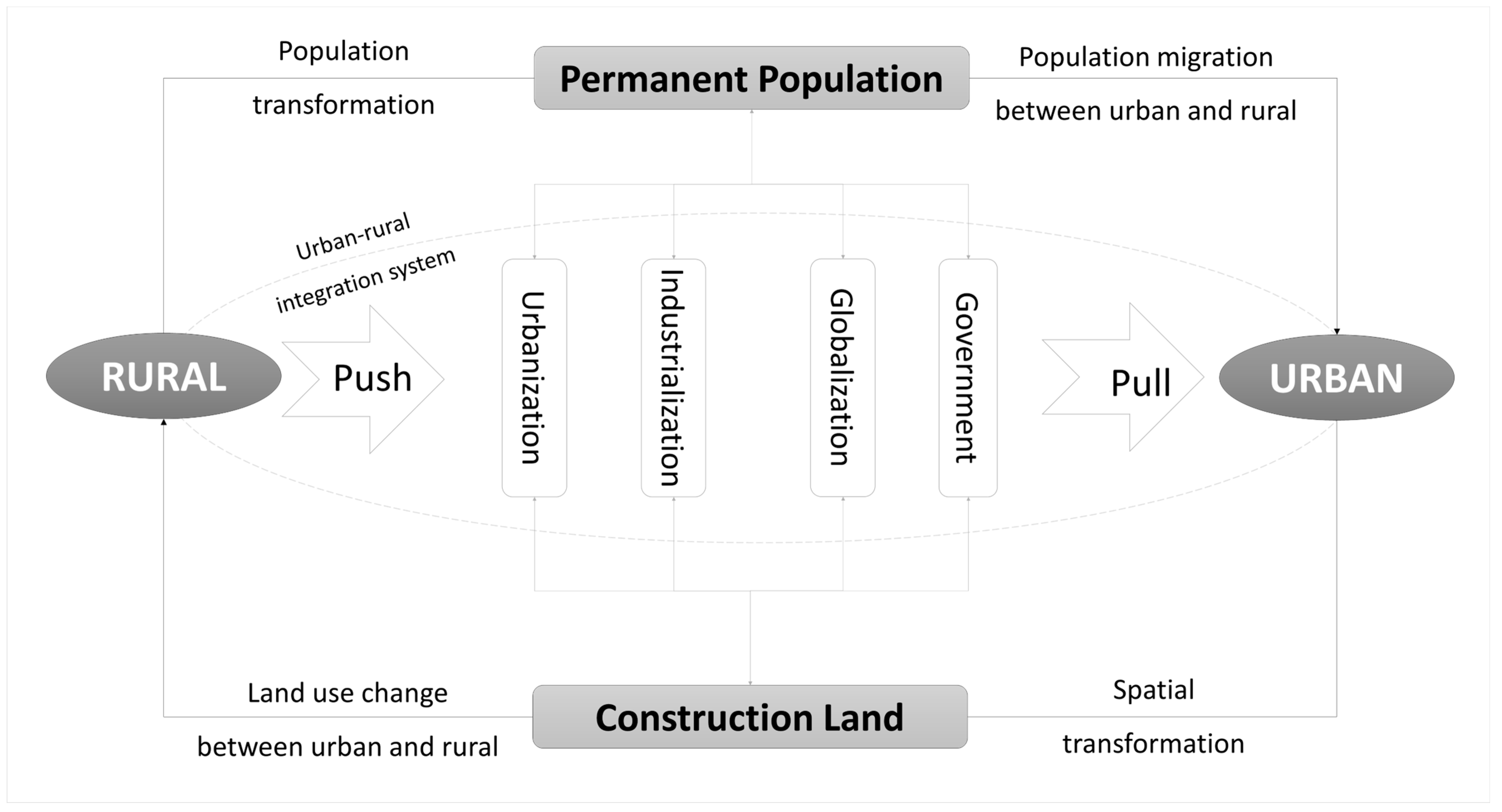
1.3. Theoretical Framework and Research Hypotheses

The relationship between construction land use and permanent population is a dynamic structure formed by the interconnection and interaction between urban and rural areas; it is also the result of multiple factors, such as urbanization, industrialization, globalization, government demand, and policies. Urban and rural areas are mutually interdependent, and they are significantly different in terms of several dimensions, such as population, land, resources, finances, environment, society, culture, institutions, and policies; as such, completely different population–land relations may be developed in urban and rural areas. Since there is no physical separation in space, there are complex interactions between urban and rural areas in terms of the circulation of population, land, resources, and capital factors, as well as in terms of the optimization and reconfiguration of environmental, social, cultural, institutional, and policy factors. Therefore, interconnected urban and rural subsystems are integrated into a larger regional system through interaction effects (Figure 1). The following research hypotheses are proposed in this paper:
(1) In the process of population and spatial transformation, along with the migration of rural population to urban areas and according to the urban–rural land increase–decrease linkage and balance system, permanent population and construction land use in urban areas are both increasing, while they are both decreasing in rural areas, showing a reverse synergy between population and land use in urban and rural areas. That is, ideally, urban areas exhibit strong decoupling and rural areas exhibit recessive decoupling.
(2) In the formation and evolution of the interactive relationship between construction land use and permanent population in urban and rural areas, population migration and land use transition inevitably promote adaptive changes in industry and the economy, society and culture, resources and capital, and institutions and policies. That is, in the process of forming and evolving the relationship between construction land use and permanent population in urban and rural areas, as influenced by urbanization (population, space, and society), industrialization (development stage and industrial structure), globalization (international trade and investment), and government (demand and policies), the ideal decoupling relationship proposed in hypothesis (1) is deformed or deviated, leading to inconsistencies between logic and reality.
(3) The formation and evolution of the decoupling relationship between construction land use and permanent population in urban and rural areas are influenced by many factors, and different influencing factors differ significantly in terms of their action intensity and levels (key, important, and auxiliary), nature, and mechanism (direct–interactive, push–pull, and driving force), so the government, when initiating corrective actions, should introduce targeted and adaptive management and governance policies based on the appropriate driving mechanism.

2. Materials and Methods

2.1. Study Area

The study area consists of the municipality of Shanghai and all administrative regions of the Zhejiang, Jiangsu, Anhui, Henan, and Shandong provinces, including 75 cities located in the middle-lower reaches of the Yangtze River and the Yellow River (Figure 2). The municipality of Shanghai and the Anhui, Jiangsu, and Zhejiang provinces are located in the middle-lower reaches of the Yellow River, while the Henan and Shandong provinces are in the middle-lower reaches of the Yangtze River. Shanghai, Jiangsu, Zhejiang, and Shandong are the most developed regions in China, while Anhui and Henan are among the less-developed regions, with severe population loss; they serve as the economic hinterland of the former group of regions. Due to the high level of integrated development in the study area, an empirical analysis helps explain the state of human–land relations in both urban and rural areas and reveal the spatial effects, offering a reference of great value for China and even the world. Since there are still many cities for which data from the third national land survey has not yet been published, the study area is determined based on data accessibility and the completeness of the study area (an incomplete or discontinuous study area might compromise the accuracy of the analysis of spatial effects).
It is worth noting that this paper does not distinguish urban and rural areas in the process of visualizing the study area, for the following reasons. First, China has adopted a unique administrative system whereby” urban is responsible for managing rural”. In other words, the urban area consists of three parts: districts are divided into the categories of city, county, and town; the rural areas are distributed on their periphery and managed by them. Second, the speed of urban and rural development in the study area is very fast, so the geographic boundaries of urban and rural areas change frequently, and it is difficult to visualize them consistently. Finally, the high level of urban–rural integration in the study area and the overlap of urban and rural entities make it difficult to accurately distinguish and reasonably visualize the spatial scope of urban and rural areas.

2.2. Research Steps and Data Sources

In the first step, a Boston Consulting Group matrix and exploratory spatial data analysis are employed to quantitatively analyze the phenomena and the evolutionary patterns of construction land use and permanent population in the study area, as well as to reveal the dynamic characteristics and spatial effects of land and population development. In the second step, the static and dynamic coordination relationship between construction land use and permanent population in the study area is quantitatively measured based on an evaluation of population density and the decoupling model. In addition, an exploratory spatial data analysis is performed to measure the spatial effects of decoupling types. In the third step, Geodetector is used to analyze the factors influencing the decoupling relationship between construction land use and permanent population, as well as their interaction effects, and to reveal the driving mechanism of the formation of the population–land relationship. The fourth step is to construct, using an overlay analysis, an urban–rural integration-oriented spatial policy design method based on the idea of an urban–rural community; further, we propose targeted and adaptive management suggestions for zoning. Notably, from the first step to the third step of the analysis process, urban and rural areas remain independent of each other; the fourth step highlights urban and rural integration (in line with China’s urban and rural development trends and policy management guidance).
The land data used in this study come from China’s second and third national land surveys, and the data concerning population and independent variables (influencing factors) come from the provincial and municipal statistical yearbooks. In the process of data collection, the data and drawings were processed based on the administrative divisions as of 2019, with the data for Laiwu in Shandong merged with the data for Jinan, and the data for Chaohu in Anhui merged with the data for Hefei, Ma’anshan, and Wuhu at a ratio of 2:2:1. Table A1 and Table A2 provide the statistical data for urban and rural construction land use and permanent population in the study area (total standardization). The data from the second land survey are obtained from the “Land Survey Results Sharing Application Service Platform”, and the data for the third land survey are obtained from communiques issued by the municipal governments. China launched its first national land resource survey in 1984 and launched the second and third surveys in 2007 and 2017, respectively. The data from the second survey were fully released in 2013, and the data from the third survey started to be released in 2021. According to the land survey data, the land in China is divided into eight types: arable land; garden plot; forest land; grassland; wetland; land for urban, rural, industrial, and mining activities; land used for transport systems; and land used for water and water conservancy facilities. The evaluation of construction land use in this paper includes land for settlements in cities, including both urban and rural areas, as well as land for their internal transport systems, land for green space, and external land for scenic spots, enterprises, and institutions.
At present, most papers are based on remote sensing and sectoral statistics; these methods are used to carry out individual case studies of cities, provinces, and states, with few regional and general studies. In terms of data sources, most papers depend on satellite-sourced [36,37,38], remote sensing [39,40], and night-light data [41,42,43], as well as on statistics from the land administration [44,45], while few studies are based on land survey data. Most of the current studies that use national land survey data focus on arable land changes [46,47], and only Zhang conducted an exploratory study on the relationship between rural population and construction land use in China for the period 2009–2016 [48]. Given that satellite-based remote sensing and night-light data are estimated, the differences in the estimation parameters set by different scholars lead to large deviations in the estimation and analysis results. In addition, the data are generally processed by spatial gridding, which corresponds poorly with administrative districts and does not match up with the zones of authority of government units, leading to a disconnect between academic research and practical work. The departmental data match up well with the zones of government authority, but the accuracy of the data is questioned by researchers due to the influence of multi-interest groups on data collection and the preparation of statistics. The national land resource survey is jointly implemented by many of China’s government departments, and its data processing corrects and combines the results of remote sensing interpretations, departmental data, and field surveys; thus, the survey is the most authoritative and accurate among all sources of land data.
For the driving mechanism analysis, this paper analyzes the influence of different factors and the interaction effects between them by leveraging Geodetector; the decoupling relationships between construction land use and permanent population are the dependent variables ( Y i ), and indicators of economic and social development dimensions are the dependent variables ( X i ). This paper assumes that the formation and evolution of the relationship between urban and rural construction land use and permanent population are influenced by urbanization, industrialization, globalization, and the growthist governance patterns of urban governments, as they are generally seen as important driving forces of land use and population change. The urbanization rate is an internationally accepted indicator of the level of urban development, and the ratio of urban–rural resident income is a common indicator of its social effects [49,50]. Industrialization is the deep driving force of urbanization, and per capita GDP and tertiary industry proportion are the classic indicators of the level of industrial development [51]. The middle and lower reaches of the Yangtze River and Yellow River regions have long been at the forefront of China’s open development policy; thus, in this paper, we choose to use international trade and foreign direct investment to characterize the impact of globalization on the formation and change in the relationship between population and land use. Since China, as a whole, is still a developing country, it has a particularly strong need for sustainable economic development [52,53]. In addition, influenced by its special development system and pattern, urban and rural construction in China is highly dependent on “land finance” (a phenomenon of capitalization and financialization of land resources that is the key to the government’s strategy for entrepreneurial urban management and rural revitalization) [54,55]. The cities in the study area are committed to transitioning from high-speed development to high-quality development; the Chinese government has accelerated the reform of its administrative and fiscal system in recent years, and the impact of gross domestic product (GDP) and government revenue, which reflect government demand and performance assessment, on land use and population change should not be ignored (Table 1). We cannot confirm that we have considered all factors, but we have considered the important factors.

2.3. Research Methods

2.3.1. Boston Consulting Group Matrix

A Boston Consulting Group matrix, often used in business management and economics, is applied in this paper to analyze the study area in terms of the mode of evolution of permanent population and construction land use. Cities in the study area are classified into one of four categories, namely star-cities, cow-cities, question-cities, and dog-cities, based on their change speed (CS) and relative share (RS), with their average value as the threshold. Star-cities are characterized by high relative shares and growth rates of permanent population and construction land use. They have an important and well-developed position in the region and are in a rapid growth period. Cow-cities are characterized by high relative shares of permanent population and construction land use but low growth rates, and they are important in the region but are in a mature or declining stage of development. Question-cities are characterized by low relative shares of permanent population and construction land use but high growth rates. Despite their low status in the region, they have great development potential and are likely to grow into emerging regional growth poles in the future under reasonable policy guidance. Dog-cities are characterized by low relative shares and growth rates of permanent population and construction land use. They have very low development strength and potential, and interventional policies should be adopted to promote their transformation; otherwise, their development sustainability is under threat. With t representing time, which is a period of 5 years in this paper, and Z i , Z i l a s t ,   Z i b a s e , and Z i m a x representing the attribute value of i city ( L i and P i in this paper), its base-period value, end-period value, and maximum value, respectively, CS and RS are calculated as follows [56]:
C S = Z i l a s t / Z i b a s e t 1
R S = Z i Z i m a x

2.3.2. Decoupling Model

Most papers analyze the coordination relationship between population and land use change using the coupling coordination model [57], with a few based on the ratio of land consumption to population growth (according to UN SDG 11.3.1) [58,59]. The former is essentially a static analysis that does not match the real-world state of development, while the latter is an emerging and dynamic approach that still lacks value evaluation criteria. Therefore, this paper adopts the decoupling model to analyze the dynamic relationship between construction land use and permanent population. Decoupling models are commonly used in the fields of environment, ecology, and economics, and in recent years they have been introduced to the study of land use to analyze the synergy between land consumption (such as urban and rural construction land [60,61,62], urban industrial land [63], and service land [64]) and social and economic development.
The decoupling model, proposed by Tapio [65], is used in this paper to analyze the degree of coordination between permanent population levels and changes in construction land use, in order to reveal the state of development of human–land relations. According to the positive and negative values of Δ α and Δ β , decoupling is divided into 8 types (Table 2), with 0.8 and 1.2 as the thresholds for γ [66,67], where γ is the decoupling index; Δ α is the growth rate of construction land use; Δ β is the growth rate of permanent population; P i and P i + t are the total permanent population in years i and i + t , respectively; and L i and L i + t are the amounts of construction land in years i and i + t , respectively. The decoupling index is calculated as follows [68]:
γ = Δ α Δ β
Δ α = L i + t L i L i
Δ β = P i + t P i P i

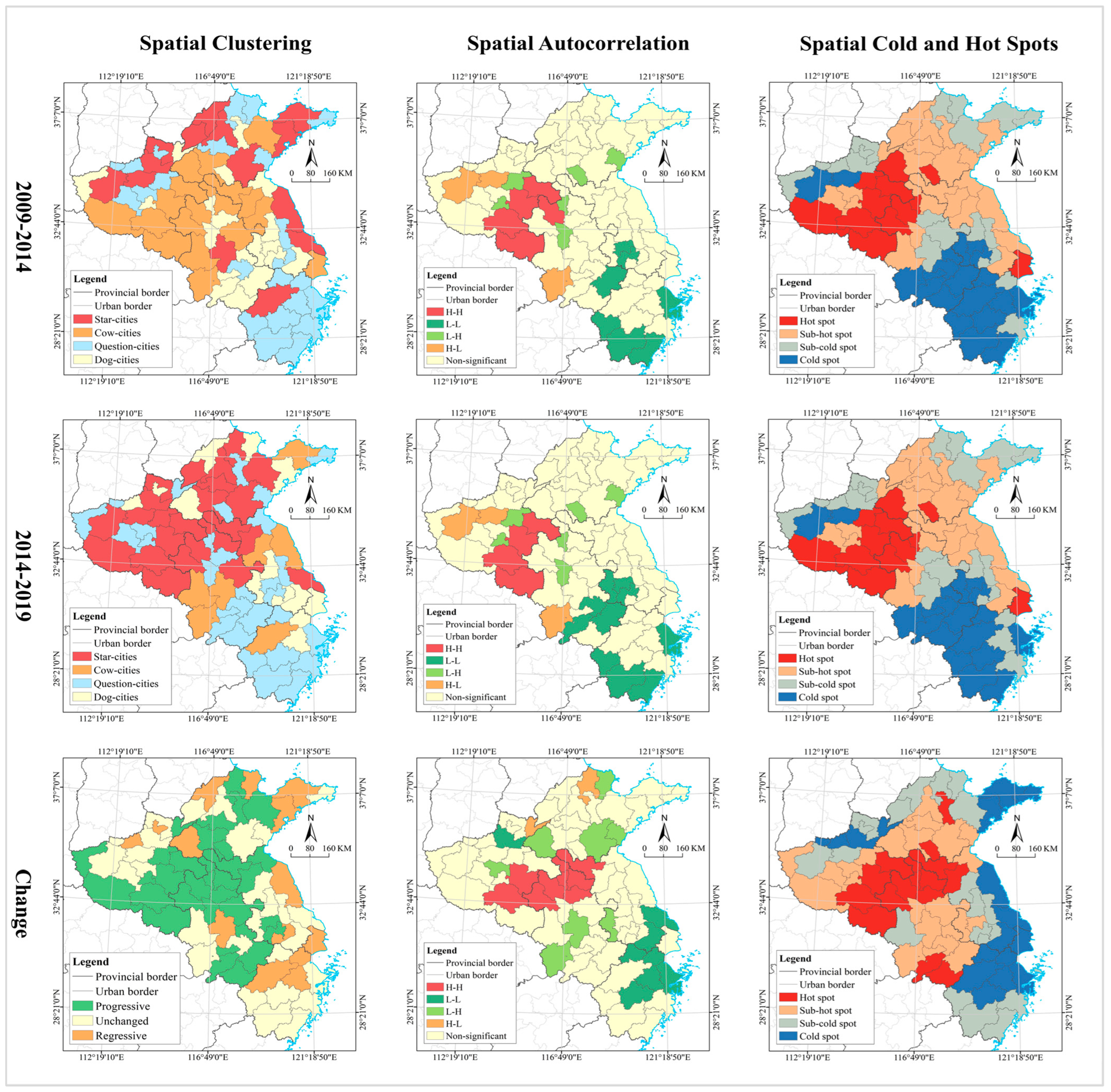
2.3.3. Exploratory Spatial Data Analysis (ESDA) and Geodetector

Before analyzing the influencing factors, the spatial effects of construction land use and permanent population, as well as their decoupling relationship, must be determined. In this paper, in case of a low level of spatial autocorrelation and heterogeneity, classical statistical regression models (such as ordinary least squares) can be used directly; otherwise, spatial regression models, such as Geodetector [69] and geographically weighted regression [70], are required. This paper analyzes the spatial effects of permanent population, construction land use, and human–land relations in urban and rural areas by adopting the ESDA approach. Cold and hot spots and spatial autocorrelation are analyzed in this paper, relying on Arcgis 10.2 and GeoDa 1.18; the significance level for the local autocorrelation analysis is 0.1, the weights are based on the spatial matrix of adjacent boundaries, and all parameters are software default values. In this paper, when the spatial effect is significant, Geodetector is used to analyze the driving mechanism because it can simultaneously analyze both the direct and interaction effects of the influencing factors, which better meets the needs of this study than the use of a geographically weighted region.
The analysis of cold and hot spots reveals incidences of clustering in geographic space of cities with high or low values [71]. A larger absolute value of Moran’s I represents a higher spatial autocorrelation. A positive global value of Moran’s I represents a positive correlation, while a negative one represents a negative correlation, and a zero value represents random distribution. The spatial associations are classified into one of four types, namely HH, HL, LH, and LL, according to the local autocorrelation analysis. HH and LL indicate positive spatial correlations, that is, the core and the periphery share the same attributes, both representing regions with high or low values, respectively. HL and LH indicate negative spatial correlations, that is, the core and the periphery have opposite attributes, representing regions of center concentration or collapse, respectively. With n representing the number of cities; M i and M j being the attribute values of cities i and j , respectively; M ¯ being the average of the attribute values, W i j being the spatial weight matrix in the global spatial autocorrelation and the row-normalized values of the spatial weights in the local spatial autocorrelation; S 0 being the sum of the spatial weight matrices; and N i and N j being the normalized values of the attributes of cities i and j , respectively, the global and local Moran’s I values are calculated as follows [72]:
Global   Moran s   I = n S 0 × i = 1 n j = 1 n W i j ( M i M ¯ ) ( M j M ¯ ) i = 1 n ( M i M ¯ ) 2 ,   S 0 = i = 1 n j = 1 n = W i j
Local   Moran s   I i = N i i = 1 n W i j N j
Geodetector was developed by Professor Wang Jinfeng and includes two versions, including one for Excel and one for the R language (http://www.geodetector.cn/, accessed on 17 September 2022). If the spatial pattern similarity between the independent variable factors ( X i ) and the dependent variables ( Y i ) is higher, Geodetector determines that X i has a greater influence on Y i [73,74]. Geodetector uses q index to characterize influence, including direct driving forces (such as q( X i ) and q( X j )) and interactive driving forces (such as q( X i X j )) of influence factors. Their values are in the range of [0, 1], and a larger value implies a greater direct and interactive influence. With h representing the number of classifications of the independent variables (h = 4 in this paper); N h and N representing the number of cities in stratum h and the study area, respectively; σ h 2 and σ 2 representing the variance of the dependent variable in stratum h and the study area, respectively; SSW representing the within sum of squares; and SST representing the total sum of squares in the study area, the calculation equation for q is as follows [75,76]:
q = 1 h = 1 l N h σ h 2 N σ 2 = 1 S S W S S T ,   S S W = h = 1 l N h σ h 2 ,   S S T = N σ 2
The interactive influence is classified into five types based on the relationship between q( X i X j ) and the minimum (Min (q( X i ), q( X j ))), maximum (Max (q( X i ), q( X j ))), and summation (q( X i ) + q( X j )) values of direct influence [77,78]. The nonlinear weaken (q( X i X j ) < Min(q( X i ), q( X j ))) and the single nonlinear weaken (Min(q( X i ), q( X j )) < q( X i X j ) < Max(q( X i ), q( X j ))) represent the antagonistic effect between different factors, indicating that the driving forces of i and j cancel each other out when they act together on Y , and that their influence is weakened or even disappears; thus, the pairing of the two factors should be avoided in policy design when possible. The bifactor enhancement (q( X i ) + q( X j ) > q( X i X j ) > Max (q( X i ), q( X j ))) and nonlinear enhancement (q( X i X j ) > q( X i ) + q( X j )) represent a synergy effect between different factors, indicating that the driving forces of i and j are mutually reinforcing when they act together on Y , and that the influence is enhanced or even significantly amplified; thus, the two factors should be paired in policy design when possible. Notably, when q( X i X j ) = q( X i ) + q( X j ), it signifies that the processes associated with the different factors are independent, and they do not interfere or relate to each other; this is a rare and special phenomenon requiring no consideration of the interactive influence in policy design; however, the direct driving force must still be considered in such instances [79,80].

3. Results

3.1. Mode of Evolution of Construction Land Use and Permanent Population

3.1.1. Urban Permanent Population

The average growth rates of urban permanent population in 2009–2014 and 2014–2019 were 4.43 and 3.04, respectively, and the average relative shares in 2014 and 2019 were 0.14 and 0.17, respectively. The distribution of the four types of cities shifted from a “pyramid”-shaped to an “olive”-shaped structure from 2009 to 2014, with a low level of clustering in geographical distribution. Star-cities accounted for 12.00%, including Suzhou (Jiangsu), Wenzhou, Hefei, Qingdao, Yantai, Jining, Linyi, Heze, and Zhengzhou. Cow-cities accounted for 21.33%, including Shanghai, Nanjing, Wuxi, Xuzhou, Changzhou, Nantong, Yancheng, Hangzhou, Ningbo, Jinhua, Taizhou (Zhejiang), Jinan, Weifang, Luoyang, Nanyang; and Zhoukou; they were relatively clustered in southern Jiangsu and the coastal areas. Question-cities accounted for 16.00%, including Lianyungang, Huai’an, Suqian, Zibo, Zaozhuang, Dongying, Tai’an, Weihai, Rizhao, Dezhou, Liaocheng, and Binzhou; they were mostly clustered in Shandong Province and northeastern Jiangsu. Dog-cities accounted for 50.67%, including Yangzhou, Zhenjiang, Taizhou (Jiangsu), Jiaxing, Huzhou, Quzhou, Bengbu, Huainan, Ma’anshan, Huaibei, Anyang, Hebi, Xinxiang, Jiaozuo, Shangqiu, Xinyang, and Jiyuan; most of them were clustered in Anhui and Henan (Figure 3).
From 2014 to 2019, about 15% were star-cities, including Hangzhou, Hefei, Fuyang, Jinan, Weifang, Jining, Heze, Zhengzhou, Luoyang, and Nanyang; they were mostly scattered in the Yellow River basin. Cow-cities accounted for 18.67%, including Shanghai, Nanjing, Wuxi, Xuzhou, Suzhou (Jiangsu), Nantong, Yancheng, Ningbo, Wenzhou, Jinhua, Taizhou (Zhejiang), Qingdao, Yantai, and Linyi; they were mainly clustered in Jiangsu, Zhejiang, and southwestern Shandong. Question-cities accounted for 36%, including Changzhou, Huai’an, Yangzhou, Zhenjiang, Shaoxing, Zhoushan, Wuhu, Huaibei, Anqing, Dezhou, Binzhou, and Jiyuan; they formed three clustered agglomerations in southwestern Anhui, central Jiangsu, and northeastern Shandong. About 30% were dog-cities, including Changzhou, Lianyungang, Huai’an, Yangzhou, Zhenjiang, Taizhou (Jiangsu), Suqian, Shaoxing, Zhoushan, Wuhu, Ma’anshan, Huaibei, Anqing, Lu’an, Chizhou, Zibo, Dongying, Tai’an, and Weihai.
The value of global Moran’s I shifted from 0.05 (p > 0.10, Z = 0.71) to −0.11 (p > 0.10, Z = −1.09), indicating a lower and positive to negative spatial autocorrelation of urban population distribution. Qingdao, Rizhao, Tai’an, Zaozhuang, and Nantong were HH-type cities from 2009 to 2014, shrinking to only Qingdao from 2014 to 2019. The hot-spot cities from 2009 to 2014 were clustered in the Shandong Peninsula and the Shanghai metropolitan area, including Weihai, Yantai, Langfang, Qingdao, Jining, Zaozhuang, Tai’an, Shanghai, Suzhou (Jiangsu), and Nantong. Most of the hot-spot cities from 2014 to 2019 were clustered in Henan, including Nanyang, Pingdingshan, Luohe, Xuchang, Kaifeng, Jiyuan, Qingdao, Shanghai, Nantong, and Taizhou (Zhejiang). The cold-spot cities from 2009 to 2014 were clustered in the Henan and Anhui provinces and shifted to central Jiangsu and northeastern Shandong from 2014 to 2019, with a significant reduction in geographical coverage.
According to the changes between the two periods, 41.33% of the cities were progressive, including Hangzhou, Jiaxing, Huzhou, Bengbu, Huainan, Tongling, Jinan, Weifang, Kaifeng, Luoyang, Xinyang, Zhoukou, and Zhumadian; they were mostly clustered in Henan, with a small number in the border area between Anhui and Zhejiang. About one-fifth of the cities were regressive, including Changzhou, Suzhou (Jiangsu), Lianyungang, Huai’an, Suqian, Wenzhou, Qingdao, Zibo, Dongying, Yantai, Tai’an, Weihai, Linyi, Dezhou, and Binzhou; they were mostly in Shandong, with a trend of extending to central Jiangsu. Unchanged cities accounted for 38.67%, including Shanghai, Nanjing, Wuxi, Xuzhou, Ningbo, Shaoxing, Jinhua, Zhoushan, Hefei, Wuhu, Ma’anshan, Zaozhuang, Jining, Rizhao, Zhengzhou, Sanmenxia, and Jiyuan; they were mostly clustered in Jiangsu; with a trend of extending to southern Anhui, eastern Zhejiang, and western Shandong. The value of global Moran’s I was 0.01 (p > 0.10, Z = 0.20), indicating a positive spatial autocorrelation of the change in the evolution mode of urban population. HH cities were clustered in Henan, including Pingdingshan, Xuchang, Luohe, Kaifeng, and Xinxiang. Binzhou, Yantai, Lianyungang, and Suqian were LL cities. Cold- and hot-spot cities showed a core-periphery and gradient structure in their geographic distribution. The hot-spot and secondary hot-spot cities were distributed in the west of the study area, covering the whole of the Henan and Anhui provinces and northern Zhejiang. The cold-spot cities were distributed in Shandong, with secondary cold spots clustered in its periphery and extending to Jiangsu.

3.1.2. Rural Permanent Population

The average growth rates of rural permanent population in 2009–2014 and 2014–2019 were −1.58 and −0.23, respectively, and the average relative shares in 2014 and 2019 were 0.37 and 0.40, respectively. The four types of cities maintained a “pyramid”-shaped structure for a long time, and they were highly clustered, with a low autocorrelation in geographical distribution. From 2009 to 2014, Shanghai, Suzhou (Jiangsu), Bozhou, Jinan, Qingdao, Weifang, Zhengzhou, and Nanyang were star-cities; Nanjing, Wuxi, Changzhou, Zhenjiang, Quzhou, Wuhu, Bengbu, Huaibei, Hebi, Puyang, and Luohe were question-cities, and were comparatively clustered in southern Jiangsu. Cow-cities accounted for 34.67%, including Xuzhou, Nantong, Yancheng, Hefei, Anqing, Lu’an, Yantai, Jining, Kaifeng, Luoyang, and Xinxiang; they were mostly clustered in the Yellow River basin. Dog-cities accounted for 40%, including Lianyungang, Huai’an, Yangzhou, Ningbo, Wenzhou, Jiaxing, Lishui, and Huainan; they were clustered in the Jiangsu and Zhejiang provinces (Figure 4).
From 2014 to 2019, Shanghai, Hangzhou, Ningbo, Wenzhou, and Linyi were star-cities, while Jiaxing, Huzhou, Shaoxing, Jinhua, Zhoushan, Huainan, and Tongling were question-cities. Cow-cities accounted for 40%, including Jinan, Qingdao, Yantai, Weifang, Jining, Tai’an, Dezhou, Liaocheng, Heze, Zhengzhou, Kaifeng, Luoyang, Anyang, Xinyang, Zhoukou, Zhumadian, Xuzhou, Suzhou (Jiangsu), Nantong, Yancheng, Taizhou (Zhejiang), Anqing, Fuyang, Suzhou (Anhui), Lu’an, and Bozhou; they were mostly clustered in Henan and Shandong, with a trend of extending to Anhui and northern Jiangsu. Dog-cities accounted for 44%, including Nanjing, Wuxi, Changzhou, Lianyungang, Huai’an, Yangzhou, Zhenjiang, Taizhou (Jiangsu), Suqian, Quzhou, Lishui, Hefei, and Wuhu; they were mostly clustered in the border area between Anhui and Jiangsu.
The value of global Moran’s I shifted from 0.22 (p < 0.05, Z = 2.58) to 0.07 (p > 0.10, Z = 0.96), reflecting the decreasing spatial autocorrelation. From 2009 to 2014, HH cities were clustered in Henan, including Shangqiu, Zhoukou, Xuchang, and Pingdingshan, but from 2014 to 2019, this group was reduced to only Taizhou in Zhejiang. LL cities from 2009 to 2014 were clustered in Zhejiang and extended to the border of the Jiangsu and Anhui provinces, including Hangzhou, Shaoxing, Jinhua, Nanjing, Zhenjiang, and Xuancheng. LL cities from 2014 to 2019 were clustered in the greater Nanjing metropolitan area, including Nanjing, Zhenjiang, Yangzhou, Changzhou, Ma’anshan, Chuzhou, and Wuhu. The hot-spot and secondary hot-spot cities were clustered in the Yellow River basin from 2009 to 2014, with the cold-spot and secondary cold-spot cities clustered in the Yangtze River basin. From 2014 to 2019, the coverage of the hot-spot cities shrank significantly to only a small cluster area in eastern Zhejiang, while the secondary hot-spot cities were still clustered in Henan. The cold-spot cities were clustered in the greater Nanjing metropolitan area, and the secondary cold-spot cities were distributed in its periphery.
According to the changes between the two periods, Hangzhou, Ningbo, Wenzhou, Jiaxing, Huzhou, Shaoxing, Jinhua, Zhoushan, Huainan, Tongling, and Linyi were progressive; they were mostly clustered in Zhejiang. Nanjing, Wuxi, Changzhou, Suzhou (Jiangsu), Zhenjiang, Quzhou, Hefei, Wuhu, Bengbu, Huaibei, Bozhou, Jinan, Qingdao, Weifang, Zhengzhou, Hebi, Puyang, Xuchang, Luohe, and Nanyang were regressive; they were scattered in their geographical distribution. Unchanged cities accounted for 58.67%, including Xuzhou, Nantong, Huai’an, Lishui, Anqing, Chuzhou, Suzhou (Anhui), Yantai, Jining, Tai’an, Kaifeng, Luoyang, Anyang, and Xinxiang. The value of global Moran’s I was 0.02 (p > 0.1, Z = 0.43), indicating a very low positive spatial autocorrelation for the change in the evolution mode of rural population. HH cities were clustered in central Zhejiang, including Hangzhou, Jinhua, Shaoxing, Jiaxing, and Ningbo, and LL cities included Nanjing, Zhejiang, and Changzhou. The geographical distribution of cold- and hot-spot cities had a core-periphery structure. Most of the hot-spot and secondary hot-spot cities were clustered in Zhejiang and extended to southwestern Anhui. The cold-spot cities were relatively isolated, while the secondary cold-spot cities were mainly clustered in the Yellow River basin and extended to the border area of Anhui and Jiangsu.

3.1.3. Urban Construction Land Use

The average growth rates of urban construction land use in 2009–2014 and 2014–2019 were 3.68 and 5.23, respectively, and the average relative shares in 2014 and 2019 were 0.11 and 0.23, respectively. The four types of cities were distributed in a “pyramid”-shaped structure, and they were spatially clustered in terms of geographical distribution. From 2009 to 2014, only Hefei and Zhengzhou were star-cities. Cow-cities accounted for 22.67%, including Shanghai, Nanjing, Wuxi, Xuzhou, Changzhou, Suzhou (Jiangsu), Nantong, Hangzhou, Ningbo, Jinhua, Jinan, Qingdao, Zibo, Yantai, Weifang, Jining, and Linyi; they were mostly clustered in southern Jiangsu and Shandong. Question-cities accounted for 37.33%, including Huai’an, Zhenjiang, Taizhou (Jiangsu), Suqian, Quzhou, Lishui, Wuhu, Bengbu, Huainan, Huaibei, Anqing, Huangshan, Chuzhou, Suzhou (Anhui), Lu’an, Bozhou, Chizhou, Xuancheng, Dongying, Binzhou, Anyang, Hebi, Puyang, Luohe, Sanmenxia, Shangqiu, Zhoukou, and Zhumadian; they were mostly clustered in Anhui as well as in southeastern Henan, northern Jiangsu, and western Zhejiang. Dog-cities accounted for 37.33%, including Lianyungang, Yancheng, Yangzhou, Wenzhou, Jiaxing, Huzhou, Shaoxing, Zhoushan, Taizhou (Zhejiang), Ma’anshan, Tongling, Fuyang, Zaozhuang, Tai’an, Weihai, Rizhao, Dezhou, Liaocheng, Heze, Kaifeng, Luoyang, Pingdingshan, Xinxiang, Jiaozuo, Xuchang, Nanyang, Xinyang, and Jiyuan; they were mostly clustered in northwestern Henan, with a small number clustered In eastern Zhejiang and the marginal area of Shandong (Figure 5).
From 2014 to 2019, star-cities accounted for 18.67%, including Wuxi, Xuzhou, Suzhou (Jiangsu), Nantong, Yancheng, Hangzhou, Jiaxing, Qingdao, Yantai, Jining, Linyi, Dezhou, Heze, and Zhengzhou, with a belt-like agglomeration in the lower reaches of the Yangtze River and a cluster-like agglomeration in the lower reaches of the Yellow River. Cow-cities accounted for 10.67%, including Shanghai, Nanjing, Changzhou, Ningbo, Jinhua, Hefei, Jinan, and Weifang; all were located in the periphery of star-cities. Question-cities accounted for 26.67%, including Yangzhou, Suqian, Huzhou, Zhoushan, Huainan, Fuyang, Bozhou, Dongying, Weihai, Rizhao, Liaocheng, Binzhou, Kaifeng, Pingdingshan, Anyang, Hebi, Puyang, Xuchang, Shangqiu, and Zhumadian; they were mostly clustered in the lower reaches of the Yellow River, especially in Henan. Dog-cities accounted for 44.00%, including Lianyungang, Huai’an, Zhenjiang, Taizhou (Jiangsu), Wenzhou, Shaoxing, Quzhou, Taizhou (Zhejiang), Lishui, Wuhu, Bengbu, Ma’anshan, Tongling, Anqing, Huangshan, Chuzhou, Suzhou (Anhui), Lu’an, Chizhou, Xuancheng, Zibo, Zaozhuang, Tai’an, Luoyang, Xinxiang, Jiaozuo, Luohe, Sanmenxia, Nanyang, Xinyang, Zhoukou, and Jiyuan; they were mostly clustered in Anhui, western Henan, and southern Zhejiang. The value of global Moran’s I shifted from −0.17 (p < 0.10, Z = −1.26) to 0.10 (p < 0.10, Z = 1.28), indicating a negative to positive spatial autocorrelation. Except for the HH cities clustered in the greater Shanghai metropolitan area from 2014 to 2019, all others were isolated in the local spatial association pattern. The hot-spot cities remained clustered in the urban agglomerations in southern Jiangsu and the Shandong Peninsula for a long time, while the cold-spot cities were scattered in Henan, Shandong, and Jiangsu in the early stages and relatively clustered in Anhui and southwestern Zhejiang in the later stages.
According to the changes between the two periods, 30.67% of the cities were progressive, including Yancheng, Jiaxing, Dezhou, Heze, Wuxi, Xuzhou, Suzhou (Jiangsu), Nantong, Yangzhou, Hangzhou, Huzhou, Zhoushan, Fuyang, Qingdao, Yantai, Jining, Weihai, Rizhao, Linyi, Liaocheng, Kaifeng, Pingdingshan, and Xuchang; they were mostly clustered in Shandong and southern Jiangsu. Regressive cities accounted for 26.67%, including Huai’an, Zhenjiang, Taizhou (Jiangsu), Quzhou, Lishui, Hefei, Wuhu, Bengbu, Huaibei, Anqing, Huangshan, Chuzhou, Suzhou (Anhui), Lu’an, Chizhou, Xuancheng, Luohe, Sanmenxia, Zhoukou, and Zibo; they were mostly clustered in Anhui and western Zhejiang. About 40% of the cities remained unchanged, including Shanghai, Nanjing, Changzhou, Lianyungang, Suqian, Ningbo, Wenzhou, Shaoxing, Jinhua, Taizhou (Zhejiang), Huainan, Ma’anshan, Tongling, Bozhou, Jinan, Zaozhuang, Dongying, Weifang, Tai’an, Binzhou, Zhengzhou, Luoyang, Anyang, Hebi, Xinxiang, Jiaozuo, Puyang, Nanyang, Shangqiu, Xinyang, Zhumadian, and Jiyuan; they were distributed in clusters in southeastern Zhejiang, northeastern Shandong, and northwestern Henan. The value of global Moran’s I was 0.22 (p < 0.05, Z = 2.57), indicating that the change in the mode of evolution had a positive spatial autocorrelation. The HH cities were Suzhou in Jiangsu and Huzhou in Zhejiang, and the LL cities were clustered in southwestern Anhui. Most of the hot-spot cities were clustered in Hangzhou Bay, the shore of Taihu Lake, and Shandong, while the cold-spot cities were clustered in southwestern Anhui.

3.1.4. Rural Construction Land Use

The average growth rates of rural construction land use in 2009–2014 and 2014–2019 were 0.72 and 1.22, respectively, and the average relative shares in 2014 and 2019 were 0.12 and 0.22, respectively. The four types of cities were distributed in an “olive”- to “inverted pyramid”-shaped structure, and they were spatially clustered in terms of geographical distribution, with largely the same spatial pattern of autocorrelation and cold and hot spots. From 2009 to 2014, star-cities accounted for 18%, including Nantong, Yancheng, Hangzhou, Hefei, Jinan, Qingdao, Yantai, Linyi, Dezhou, Liaocheng, Zhengzhou, Luoyang, Anyang, and Xinxiang; they were isolated in geographical distribution. Cow-cities accounted for 24.00%, including Shanghai, Xuzhou, Huai’an, Suqian, Anqing, Chuzhou, Fuyang, Suzhou (Anhui), Lu’an, Bozhou, Weifang, Jining, Heze, Nanyang, Shangqiu, Xinyang, Zhoukou, and Zhumadian; they were mostly clustered in the border areas of Henan, Anhui, and Jiangsu. Question-cities accounted for 32.00%, including Wuxi, Taizhou (Jiangsu), Ningbo, Wenzhou, Jiaxing, Huzhou, Shaoxing, Jinhua, Quzhou, Zhoushan, Taizhou (Zhejiang), Lishui, Wuhu, Dongying, Tai’an, Weihai, Rizhao, Binzhou, Kaifeng, Pingdingshan, Hebi, Jiaozuo, and Xuchang; they were mostly clustered in Zhejiang. A quarter were dog-cities, including Nanjing, Changzhou, Suzhou (Jiangsu), Lianyungang, Yangzhou, Zhenjiang, Bengbu, Huainan, Ma’anshan, Huaibei, Tongling, Huangshan, Chizhou, Xuancheng, Zibo, Zaozhuang, Puyang, Luohe, and Sanmenxia; they were relatively clustered in Jiangsu and southern Anhui (Figure 6).
About one-third were star-cities from 2014 to 2019, including Xuzhou, Nantong, Suqian, Chuzhou, Fuyang, Suzhou (Anhui), Bozhou, Jinan, Weifang, Jining, Tai’an, Linyi, Liaocheng, Binzhou, Zhengzhou, Kaifeng, Luoyang, Anyang, Xinxiang, Nanyang, Shangqiu, Xinyang, Zhoukou, and Zhumadian; they were mostly clustered in the Yellow River basin. About 10% were cow-cities, including Huai’an, Yancheng, Hangzhou, Hefei, Anqing, and Lu’an; they were scattered in Anhui and Jiangsu. Question-cities accounted for 41.33%, including Changzhou, Lianyungang, Zhenjiang, Wenzhou, Huzhou, Jinhua, Quzhou, Zhoushan, Taizhou (Zhejiang), Lishui, Wuhu, Bengbu, Huainan, Ma’anshan, Huaibei, Tongling, Huangshan, Chizhou, Xuancheng, Zibo, Zaozhuang, Weihai, Rizhao, Pingdingshan, Puyang, Xuchang, Luohe, and Jiyuan; they were mostly clustered in the Anhui–Zhejiang border area and southern Zhejiang. About 20% were dog-cities, including Shanghai, Nanjing, Wuxi, Suzhou (Jiangsu), Yangzhou, Jiaxing, Shaoxing, Qingdao, Dongying, Dezhou, Heze, Hebi, and Jiaozuo. The value of global Moran’s I shifted from −0.04 (p > 0.10, Z = −0.21) to −0.01 (p > 0.10, Z = 0.05), indicating a decreasing negative spatial autocorrelation despite it being no statistical significance. HH cities remained clustered along the border area between Anhui and Henan, while LL cities were mostly clustered in southern Zhejiang and the Anhui–Zhejiang–Jiangsu junction areas. The hot-spot and secondary hot-spot cities remained clustered in the Yellow River basin, especially in Henan; the cold-spot and secondary cold-spot cities remained clustered in the Yangtze River basin, especially in Zhejiang.
From the changes between the two periods, 42.67% of the cities were progressive, including Tai’an, Binzhou, Kaifeng, Xuzhou, Changzhou, Lianyungang, Zhenjiang, Suqian, Bengbu, Huainan, Ma’anshan, Huaibei, Tongling, Huangshan, Chuzhou, Fuyang, Suzhou (Anhui), Bozhou, Chizhou, Xuancheng, Zibo, Zaozhuang, Weifang, Jining, Puyang, Luohe, Sanmenxia, Nanyang, Shangqiu Xinyang, Zhoukou, and Zhumadian; they were mostly clustered in the Yellow River basin, extending to northern Anhui and Jiangsu in the Yangtze River basin. About one-fifth of the cities were regressive, including Wuxi, Yancheng, Hangzhou, Jiaxing, Shaoxing, Hefei, Dongying, Yantai, Hebi, Jiaozuo, Shanghai, Heze, Qingdao, and Dezhou; they were isolated in geographical distribution. Unchanged cities accounted for 38.67%, including Nanjing, Suzhou (Jiangsu), Nantong, Huai’an, Yangzhou, Taizhou (Jiangsu), Ningbo, Wenzhou, Huzhou, Jinhua, Quzhou, Zhoushan, Taizhou (Zhejiang), Lishui, Wuhu, Lu’an, Jinan, Weihai, Rizhao, Linyi, Liaocheng, Zhengzhou, Luoyang, Pingdingshan, Anyang, Xinxiang, Xuchang, and Jiyuan; they were mostly clustered in the Zhejiang and Jiangsu provinces in the Yangtze River basin, with a small number in northern Henan in the Yellow River basin. The value of global Moran’s I was 0.22 (p < 0.05, Z = 2.67), indicating that the change in the mode of evolution had a positive spatial autocorrelation. HH cities were clustered in southern Henan and the Huaihai Economic Zone, while LL cities were clustered in the Zhejiang–Jiangsu border area. The geographical distribution of cold- and hot-spot cities had a core-periphery structure. Most of the hot-spot and secondary hot-spot cities were clustered in the Yellow River basin, especially in Henan, and they extended to Anhui. The cold-spot cities were clustered in Hangzhou Bay and the Shandong Peninsula, with the secondary cold-spot cities distributed in their periphery and extending inland to Henan.

3.2. Decoupling Analysis between Construction Land Use and Permanent Population

3.2.1. Urban Decoupling Relationship

From 2009 to 2014, 44.00% of the cities were in a state of weak decoupling, including Wuxi, Xuzhou, Suzhou (Jiangsu), Nantong, Lianyungang, Yancheng, Suqian, Hangzhou, Ningbo, Wenzhou, Jiaxing, Huzhou, Taizhou (Zhejiang), Hefei, Jinan, Qingdao, Zibo, Zaozhuang, Dongying, Yantai, Weifang, Jining, Tai’an, Weihai, Rizhao, Linyi, Dezhou, Liaocheng, Binzhou, Heze, Xinxiang, Jiaozuo, and Jiyuan; they were mostly clustered in the east of the study area, especially in Shandong, and they extended along the coastline to the Jiangsu and Zhejiang provinces. About 18.67% of the cities were in a state of expansive coupling, including Shanghai, Changzhou, Huai’an, Yangzhou, Taizhou (Jiangsu), Shaoxing, Jinhua, Zhoushan, Zhengzhou, Luoyang, Pingdingshan, Xuchang, Luohe, and Xinyang; they were scattered in the Jiangsu and Henan provinces. About 36.00% of the cities were in a state of expansive negative decoupling, including Nanjing, Zhenjiang, Quzhou, Lishui, Wuhu, Bengbu, Huainan, Huaibei, Tongling, Anqing, Huangshan, Chuzhou, Fuyang, Suzhou (Anhui), Lu’an, Bozhou, Chizhou, Xuancheng, Kaifeng, Anyang, Hebi, Puyang, Sanmenxia, Nanyang, Shangqiu, Zhoukou, and Zhumadian; they were mostly clustered in the west of the study area, especially in Anhui and Henan, which are two less-developed provinces. In summary, human–land relations in urban areas were generally reasonable, with more than 60% of cities in a state of either weak decoupling or expansive coupling. Significantly, more than one-third of the cities were still in a state of expansive negative decoupling, especially Ma’anshan, a city in strong negative decoupling, with an extensive or even wasteful use of land and unreasonable human–land relations, which are factors that may block sustainable urban development. From 2014 to 2019, Wuhu, Ma’anshan, Anqing, Huangshan, and Chizhou were in a state of strong decoupling; they were clustered in southern Anhui. Shanghai and Lu’an were in a state of recessive decoupling, with reasonable human–land relations, but the urban areas were in a shrinking phase, which constrained sustainable development. There were an equal number of cities in states of weak decoupling and expansive coupling, with the former including Lianyungang, Quzhou, Hefei, Bengbu, Huainan, Huaibei, Tongling, Xuancheng, Jinan, Zibo, Sanmenxia, and Jiyuan, and the latter including Zhenjiang, Ningbo, Lishui, Chuzhou, Suzhou (Anhui), Weifang, Luoyang, Xinxiang, Luohe, Nanyang, Xinyang, and Zhoukou. It should be noted that 58.67% of the cities were in a state of expansive negative decoupling, with sloppy land resource utilization and unreasonable human–land relations. These cities were widely distributed in the Zhejiang, Jiangsu, Shandong, and Henan provinces, and they included Nanjing, Wuxi, Xuzhou, Changzhou, Suzhou (Jiangsu), Nantong, Huai’an, Yancheng, Yangzhou, Taizhou (Jiangsu), Suqian, Hangzhou, Wenzhou, Jiaxing, Shaoxing, Jinhua, Zhoushan, Fuyang, Bozhou, and Qingdao (Figure 7).
From 2009 to 2014, the value of global Moran’s I was 0.43 (p < 0.05, Z = 5.08), indicating a positive spatial autocorrelation for human–land relations. Most of the HH cities were clustered in Shandong and extended to Jiangsu, with a small number clustered in Henan and central Zhejiang, including Dezhou, Jinan, Zibo, Tai’an, Linyi, Rizhao, Lianyungang, Huai’an, Yangzhou, Taizhou (Jiangsu), Suzhou (Jiangsu), Shanghai, Jinhua, Shaoxing, Zhoushan, Zhengzhou, Xuchang, Pingdingshan, and Luoyang. LL cities were clustered in eastern Anhui and southern Henan, including Chizhou, Tongling, Wuhu, Ma’anshan, Chuzhou, Suzhou (Anhui), Nanjing, Zhumadian, Luohe, and Zhoukou. The hot-spot and secondary hot-spot cities were clustered in the east of the study area, especially in the Shandong Peninsula and Hangzhou Bay. The cold-spot and secondary cold-spot cities were clustered in the west of the study area, especially in the border area between the Anhui and Jiangsu provinces. From 2014 to 2019, the value of global Moran’s I was 0.33 (p < 0.05, Z = 3.76), indicating that the spatial pattern of human–land relations still had positive autocorrelation, but the spatial correlation and dependence were decreasing. Most of the HH cities were clustered in the south of Anhui, including Anqing, Chizhou, Tongling, Wuhu, Ma’anshan, Huangshan, Xuancheng, and Chuzhou. LL cities were distributed in the periphery of the Shanghai metropolitan area, including Nantong, Suzhou (Jiangsu), and Jiaxing. The hot-spot cities were clustered in southern Anhui, and most of the secondary hot-spot cities were clustered in Anhui, central Shandong, and northwestern Henan. The cold-spot cities were clustered in the border areas between the Jiangsu, Henan, and Shandong provinces, with the secondary cold spots distributed in their periphery (Figure 8).

3.2.2. Rural Decoupling Relationship

From 2009 to 2014, 66.67% of the cities were in a state of strong negative decoupling, mostly clustered in the Yellow River basin, with a small number in eastern Jiangsu and Zhejiang in the Yangtze River basin. About 18.67% of the cities were in a state of weak negative decoupling, including Xuancheng, Suzhou (Anhui), Ma’anshan, Lu’an, Lianyungang, Huangshan, Huainan, Huaibei, Huai’an, Chuzhou, Chizhou, Bozhou, Bengbu, and Anqing; they were mostly clustered in Anhui. Wuhu, Shanghai, Qingdao, and Hebi were in a state of expansive negative decoupling, while Zhenjiang, Nanjing, and Changzhou were in a state of strong decoupling, and Zhengzhou, Wuxi, Suzhou (Jiangsu), and Jinan were in a state of weak decoupling. To sum up, human–land relations in rural areas were not reasonable, with about 90% of cities in a state of negative decoupling. From 2014 to 2019, only Shanghai was in a state of strong decoupling, while Hangzhou, Ningbo, Wenzhou, Jiaxing, Shaoxing, Jinhua, and Zhoushan were in a state of weak decoupling. These cities had reasonable human–land relations, and most of them were clustered in Zhejiang. Tongling was in a state of expansive coupling. Nanjing, Wuxi, Qingdao, Dezhou, and Heze were in a state of recessive decoupling, with unsustainable development of human–land relations. Huzhou, Huainan, and Linyi were in a state of expansive negative decoupling; Suzhou (Jiangsu), Hefei, Anqing, Lu’an, and Dongying were in a state of weak negative decoupling; Xuzhou, Changzhou, Nantong, Lianyungang, Huai’an, Yancheng, Lishui, Wuhu, Bengbu, Ma’anshan, Huangshan, Chuzhou, Weihai, Rizhao, Liaocheng, Binzhou, Zhengzhou, Kaifeng, and Luoyang were in a state of strong negative decoupling; they were clustered in the Henan, Jiangsu, Anhui, and Shandong provinces (Figure 9).
From 2009 to 2014, the value of global Moran’s I was 0.21 (p < 0.05, Z = 2.47), indicating a positive spatial autocorrelation for human–land relations. HH cities were clustered in southern Jiangsu, including Nanjing, Zhenjiang, Changzhou, Wuxi, and Suzhou (Jiangsu). LH cities were distributed in the periphery of HH cities, and there was only one LL city, namely Zhoukou in Henan. The hot-spot and secondary hot-spot cities were clustered in Jiangsu in a core-periphery structure, and the cold-spot cities were distributed in the south and center of the study area, including the Jiangsu–Anhui–Henan–Shandong border areas and in Zhejiang province. From 2014 to 2019, the value of global Moran’s I was 0.39 (p < 0.05, Z = 4.55), indicating that the spatial pattern of human–land relations still had a positive autocorrelation, with increasing spatial correlation and dependence. Most of the HH cities were clustered in Zhejiang, including Hangzhou, Huzhou, Jiaxing, Shaoxing, and Jinhua. The hot-spot cities were clustered in Hangzhou Bay, with secondary hot-spot cities distributed in its periphery and extending to Anhui. The cold-spot cities were clustered in Henan and extended to Jiangsu. Most of the secondary cold-spot cities were clustered in Shandong, with a small number clustered in Anhui (Figure 10).

3.2.3. Changing Trends in the Decoupling Relationships in Urban and Rural Areas

For urban areas, about one-fourth of the cities in the study area were progressive, including Ma’anshan, Wuhu, Anqing, Huangshan, Chizhou, Quzhou, Bengbu, Huainan, Huaibei, Tongling, Xuancheng, Sanmenxia, Zhenjiang, Lishui, Chuzhou, Suzhou (Anhui), Nanyang, and Zhoukou; they were mostly clustered in southern and eastern Anhui. About one-fifth of the cities remained unchanged, including Nanjing, Lianyungang, Hefei, Fuyang, Bozhou, Jinan, Zibo, Kaifeng, Luoyang, Anyang, Hebi, Puyang, Luohe, Shangqiu, Xinyang, Zhumadian, and Jiyuan; they were mostly in Henan. About 53.33% of the cities were regressive, including Changzhou, Huai’an, Yangzhou, Taizhou (Jiangsu), Ningbo, Shaoxing, Jinhua, Zhoushan, Weifang, Zhengzhou, Xuchang, Wuxi, Xuzhou, Suzhou (Jiangsu), Nantong, Yancheng, Suqian, Hangzhou, Wenzhou, Jiaxing, Huzhou, Weihai, Rizhao, Linyi, Dezhou, Liaocheng, Binzhou, Heze, and Jiaozuo; they were clustered in a continuous distribution in the east of the study area. The value of global Moran’s I was 0.49 (p < 0.05, Z = 5.35), indicating a positive spatial autocorrelation for human–land relations. Most of the HH cities were clustered in Anhui, including Huangshan, Chizhou, Anqing, Tongling, Wuhu, Ma’anshan, Hefei, Chuzhou, Bengbu, and Bozhou. LL cities were clustered in Hangzhou Bay, including Ningbo, Shaoxing, Jiaxing, Suzhou (Jiangsu), and Nantong. The hot-spot and secondary hot-spot cities were clustered in Anhui, while the cold-spot cities were distributed in the coastal area, with secondary cold-spot cities distributed in its periphery and extending to Henan (Figure 11).
For rural areas, 21.33% of the cities were progressive, including Shanghai, Hangzhou, Ningbo, Wenzhou, Jiaxing, Huzhou, Shaoxing, Jinhua, Zhoushan, Hefei, Huainan, Tongling, Dongying, Linyi, Dezhou, and Heze; they were relatively clustered in Zhejiang. About 50.67% of the cities remained unchanged, including Xuzhou, Nantong, Yancheng, Yangzhou, Taizhou (Jiangsu), Suqian, Quzhou, Taizhou (Zhejiang), Lishui, Anqing, Fuyang, Lu’an, Zibo, Zaozhuang, Yantai, Weifang, Jining, Binzhou, and Kaifeng; they were mostly clustered in the Henan, Shandong, and Jiangsu provinces. About 28.00% of the cities were regressive, including Nanjing, Wuxi, Changzhou, Suzhou (Jiangsu), Lianyungang, Huai’an, Zhenjiang, Wuhu, Bengbu, Ma’anshan, Huaibei, Huangshan, Chuzhou, Suzhou (Anhui), Bozhou, Chizhou, Xuancheng, Jinan, Qingdao, Zhengzhou, and Hebi; they were clustered in the central study area (the border area between Anhui and Jiangsu provinces). The value of global Moran’s I was 0.25 (p < 0.05, Z = 2.73), indicating a positive spatial autocorrelation for human–land relations. Most of the HH cities were clustered in Zhejiang, including Hangzhou, Jiaxing, Shaoxing, Jinhua, and Lishui. LL cities were clustered in the northern Anhui economic zone and the Nanjing metropolitan area, including Bengbu, Suzhou (Anhui), Huaibei, Bozhou, Nanjing, Zhenjiang, and Changzhou. Most of the hot-spot cities were clustered in Zhejiang, with secondary hot-spot cities distributed in Henan, the marginal area of Shandong, and western Anhui. The cold-spot cities were clustered in northern Anhui and southern Jiangsu, with secondary cold-spot cities clustered in Jiangsu and eastern Henan, southern Anhui, and the Shandong Peninsula (Figure 12).

3.3. Driving Mechanisms of Construction Land Use, Permanent Population, and Their Relationship

3.3.1. Influencing Factors

Urban construction land use and permanent population were in a coordinated relationship, in general, with most cities in a state of either weak decoupling or expansive negative decoupling, and the geographical distribution of different types of population–land decoupling relationships showed a significant positive spatial autocorrelation, with a gradient change from coastal to inland. Government demand, globalization, and industrialization were important driving forces of the decoupling relationship between urban construction land use and permanent population; these forces also influenced the formation of their spatial patterns, with urbanization being a lesser driver. It should be noted that the influence of the different factors varied widely, and that the direct driving forces were all less significant in 2014–2019 than in 2009–2014, which was consistent with the trend of the degradation of the decoupling relationship and the weakening of the spatial effect. Gross domestic product (GDP) and government revenue have long played a key role in the formation of the population–land decoupling relationship, and they were well ahead of other factors in terms of significance as a direct driving force. International trade and per capita GDP were stronger direct driving forces in the long run, while foreign direct investment and the ratio of urban–rural resident income were less significant. The direct influence of the tertiary industry proportion and the urbanization rate was high in 2009–2014 but weakened significantly in 2014–2019, especially in that the latter degraded to a point where it could not pass the significance test (Table 3).
The relationship between rural construction land use and permanent population was generally unreasonable, and most cities were in a state of either strong negative decoupling or weak negative decoupling, with an increasing positive spatial autocorrelation and a geographic distribution pattern characterized by “core–periphery” clustering. The influencing factors driving the decoupling relationship between rural construction land use and permanent population, which also drove the formation of its spatial pattern, exhibited significant differences in different periods, and the various driving forces showed trends of increase, decrease, and stability. From 2009 to 2014, urbanization remained a key driving force; in particular, the influence of the urbanization rate was far ahead in significance compared to other factors, and the influence of the ratio of urban–rural resident income should not be ignored. Moreover, industrialization (per capita GDP and tertiary industry proportion) and globalization (international trade and foreign direct investment) were in the second tier, with essentially the same impact. The direct driving force of government demand (gross domestic product and government revenue) was so weak that it can be largely ignored. The urbanization rate was still a top influencing factor from 2014 to 2019, but its role as a direct driving force saw a significant decrease. On the contrary, the influence of gross domestic product and government revenue soared rapidly; this was closely related to the implementation of the rural revitalization strategy. For example, in recent years, the central government required cities to steadily increase the proportion of land transfer revenue used for agriculture and rural areas. In particular, the Opinions on Adjusting and Improving the Use of Land Transfer Revenue (Core of Government Revenue) to Support Rural Revitalization on a Priority Basis clearly states that the proportion should reach over 50% by 2025. From 2009–2014 to 2014–2019, the influence of per capita GDP and foreign direct investment gradually increased, while the significance of the ratio of urban–rural resident income and tertiary industry proportion as driving forces decreased; international trade basically remained stable.

3.3.2. Interaction Effects

The interaction effects between the different factors are characterized by bifactor enhancement and nonlinear enhancement, with the latter showing a decreasing proportion over time. Table 4, Table 5, Table 6 and Table 7 show the results of the interaction effect analysis. The factor pairs that were in a state of nonlinear enhancement from 2009–2014 to 2014–2019 decreased from 60.71% to 46.43% for urban areas and from 53.57% to 32.14% for rural areas. Notably, the interaction effects of some factor pairs remained nonlinearly enhanced in the long run, especially X 4 X 6 (tertiary industry proportion ∩ gross domestic product) and X 2 X 7 (urban–rural resident income ratio ∩ gross domestic product); these were the same for both urban and rural areas. For urban areas, the factor pairs included X 1 X 7 (urbanization rate ∩ gross domestic product), X 2 X 7 (urban–rural resident income ratio ∩ gross domestic product), X 3 X 6 (per capita GDP ∩ foreign direct investment), X 3 X 7 (per capita GDP ∩ gross domestic product), X 3 X 8 (per capita GDP ∩ government revenue), X 4 X 6 (tertiary industry proportion ∩ foreign direct investment), X 5 X 6 (international trade ∩ foreign direct investment), X 6 X 7 (foreign direct investment ∩ gross domestic product), and X 6 X 8 (foreign direct investment ∩ government revenue). For rural areas, the factor pairs included X 2 X 3 (urban–rural resident income ratio ∩ per capita GDP), X 2 X 4 (urban–rural resident income ratio ∩ tertiary industry proportion), X 2 X 6 (urban–rural resident income ratio ∩ foreign direct investment), X 2 X 7 (urban–rural resident income ratio ∩ gross domestic product), X 2 X 8 (urban–rural resident income ratio ∩ government revenue), and X 4 X 6 (tertiary industry proportion ∩ foreign direct investment).
Although the interaction effects between factors were all synergistic (i.e., non-antagonistic), the enhancement extent varied widely among factor pairs, and the trends were not the same between urban and rural areas. For urban areas, the maximum and minimum values of the factor pair interaction effects were 0.8046 ( X 3 X 8 , per capita GDP ∩ government revenue) and 0.0713 ( X 1 X 2 , urbanization rate ∩ urban–rural resident income ratio), respectively. The average enhancement of the interaction effect of the factor pairs from 2009 to 2014 had maximum and minimum values of 0.1590 (per capita GDP) and 0.3003 (government revenue), respectively; the maximum and minimum values changed to 0.1794 (foreign direct investment) and 0.1118 (tertiary industry proportion), respectively, from 2014 to 2019. For rural areas, the maximum and minimum values of the factor pair interaction effects were 0.8293 ( X 1 X 2 , urbanization rate ∩ urban–rural resident income ratio) and 0.0713 ( X 7 X 8 , gross domestic product ∩ government revenue), respectively. The maximum and minimum values of the interaction effect of the factor pairs during 2009–2014 were 0.2962 (foreign direct investment) and 0.0923 (urbanization rate), respectively, and changed to 0.4221 (urban–rural resident income ratio) and 0.1027 (urbanization rate), respectively, in 2014–2019. A comparison of the average enhancement of the interaction effect of the factor pairs between the periods 2009–2014 and 2014–2019 shows that, for urban areas, all impact factors were reduced, but the results were much more complicated for rural areas. For urbanization rate, urban–rural resident income ratio, and tertiary industry proportion, the interaction effect of the factor pairs experienced a further increase in the enhancement effect, while per capita GDP, international trade, foreign direct investment, gross domestic product, and government revenue saw decreases of varying degrees (Table 8). Influencing factors could be seen as super interaction factors if they had a high average increase in interaction effects with other factors with a large number in a non-linear interaction relationship. For urban areas, urbanization rate, per capita GDP, international trade, and foreign direct investment were super interaction factors from 2009 to 2014; however, only urban–rural resident income ratio and foreign direct investment met this criterion in urban areas from 2014 to 2019. For rural areas, urban–rural resident income ratio, international trade, and foreign direct investment were super interaction factors in 2009–2014, while urban–rural resident income ratio and tertiary industry proportion were super interaction factors in 2014–2019.

3.3.3. Mechanism Analysis

Urban and rural areas have remained closely connected to each other for a long time, and each has influenced and co-evolved with the other, resulting in many commonalities in the mechanisms that drive the formation and evolution of their population–land relationships. The factors that drove the formation and evolution of the decoupling relationship between urban and rural construction land use and permanent population can all be classified into three types based on the strength of their direct driving forces and the interaction effects of the influencing factors. First, key factors had a very strong direct driving force. For example, the influence of gross domestic product and government revenue on the decoupling relationship between urban population and land use was more than approximately double that of the other factors; these two were the leaders among all the influencing factors. Second, influencing factors with very strong interaction effects but very weak direct driving forces were auxiliary factors. For example, foreign direct investment and urban–rural resident income ratio were long-running super interaction factors for urban and rural areas, respectively, and both were also auxiliary factors. They unleashed and exerted greater influence by activating nonlinear enhancement effects by combining with other influencing factors. Third, influencing factors that were not in an extreme state (either maximum or minimum) as either a direct driving force or an interaction effect played a vital supporting role in the long run, and they are classified as important factors. For example, for both urban and rural areas, the direct driving force of per capita GDP had a value around the average in the long run, and its interaction effects cannot be ignored, so it is regarded as a stable and important factor (Figure 13).
Since urban and rural areas are essentially separate entities of a very different nature, the mechanisms that drive the formation and changes in their population–land relations are also quite different. First, the compositions of key, important, and auxiliary factors differ significantly between urban and rural areas. For example, in urban areas, gross domestic product and government revenue were long-running key factors; however, for rural areas, they were auxiliary factors in the early stages and recently rose to the status of key factors with the implementation of the rural revitalization strategy and land finance reform. Second, when comparing urban and rural areas, the driving forces of urbanization, industrialization, globalization, and government demand consisted of different influencing factors, and their roles in the operation of the driving mechanism had large differences. The government demand force, consisting of gross domestic product and government revenue, was highly synchronized and had long been a key factor for urban areas; for rural areas, it maintained common changes in the shift from auxiliary factor to key factor. The driving mechanisms for other factors, such as urbanization, industrialization, and globalization, on the contrary, showed significant differences, which must be addressed in a targeted and adaptive way through policy design, with different objects and time periods taken into account. For example, industrialization, which is represented by per capita GDP and tertiary industry proportion, was a driving mechanism for urban areas, while globalization, represented by international trade and foreign direct investment, was a driving mechanism for rural areas. However, for rural areas, per capita GDP remained an important factor, whereas the tertiary industry proportion was reduced to an auxiliary factor. Therefore, the impact of per capita GDP should be highlighted in both urban and rural areas in terms of policy design, and common proposals can be adopted; however, the influence of tertiary industry proportion on urban and rural areas must be designed with differentiated paths to ensure its maximum value in accordance with local conditions.

4. Discussion

4.1. The Complex Relationship between Theoretical Logic and Practical Reality

According to theoretical logic, the growth of the urban permanent population and the decrease in the rural permanent population, along with urbanization, are inevitable processes and objective needs [81]. In the practical world, the development reality of most cities in the study area is consistent with the theoretical logic; however, it is worth noting that some cities have deviated from this or even completely reversed course. In this study, a total of 82.67% of the regions conformed to the logical consensus, including Nanjing, Wuxi, Xuzhou, Changzhou, Suzhou (Jiangsu), Lishui, Hefei, Wuhu, Bengbu, Jinan, Qingdao, Zibo, Zaozhuang, Dongying, Yantai, Hebi, Xinxiang, Jiaozuo, Puyang, Xuchang, Luohe, Sanmenxia, and Nanyang; these regions exhibited reasonable population changes. Shanghai, as the most developed region in China, was the first in the country to implement a policy of reduced development. Shanghai has vigorously implemented the new town development and rural revitalization strategies in recent years, basically achieving the integrated development of urban and rural public services. Therefore, it is reasonable for Shanghai’s urban population to decrease and its rural population to increase, conforming to the guidance of Shanghai’s urban and rural development planning and spatial governance policies. Both the urban and rural populations in Lu’an have declined, reflecting a serious population exodus and an irrational population decrease, which has been a new threat to sustainable development. It is of note that Hangzhou, Ningbo, Wenzhou, Jiaxing, Huzhou, Shaoxing, Jinhua, Zhoushan, Huainan, Tongling, and Linyi have seen increases in both the urban and rural populations, but whether these increases are reasonable requires further analysis. Hangzhou, Ningbo, Wenzhou, Jiaxing, Huzhou, Shaoxing, and Tongling have high levels of urban–rural integration, and their population changes are reasonable due to the construction of the Shanghai, Nanjing, Hangzhou, and Hefei metropolitan areas. Jinhua, Zhoushan, Huainan, and Linyi are less developed, and they are still at the stage of rapid urbanization. The fact that the rapid growth of the urban population is accompanied by an increase in the rural population instead of a decrease indicates that it is hard for them to rely on their own strength to achieve reasonable changes in the urban and rural populations. For that reason, they should promote local urbanization and enhance the agglomeration of the rural population in urban areas; moreover, in the future, they should focus on urbanization in different places and provide services for migrant workers by improving employment services, enhancing skills training, offering transportation and convenient travel options, facilitating applications for licenses, bettering living conditions, guaranteeing the schooling of children, and caring for left-behind children and women, so as to drive the urbanization of the rural population in the region in line with the strength exhibited in other cities (Figure 14).
Limiting and controlling land consumption to conform to ideal conditions is the priority goal of urban and rural land use. The growth in urban construction land area and the decrease in rural construction land area, along with land urbanization, are in line with the theoretical logic. The supply of urban and rural construction land should not exceed the demand, otherwise, it may lower the efficiency of land use and, thus, put arable land and ecological security under threat [82]. It is worth noting that only a few cities in the study area had a development reality consistent with the theoretical logic, and the situation in most cities was different or even completely opposite. In the study area, only Nanjing, Wuxi, Suzhou (Jiangsu), Hefei, Qingdao, Dongying, Dezhou, and Heze were in a reasonable state, with urban and rural construction land changes in line with the aforementioned logic. In Wuhu, Ma’anshan, Huangshan, and Chizhou, the amount of land for urban construction decreased, but it increased in rural areas, resulting in “reverse urbanization”, which failed to match the desired development stage and indicated unreasonable land changes. Although the amount of urban and rural construction land in Shanghai, Anqing, and Lu’an were reduced, only Shanghai took the initiative to reduce it, which is reasonable; however, the reductions in Anqing and Lu’an were the result of marginalization and not sustainable. The amount of urban and rural construction land increased in 80% of the regions, including Changzhou, Xuzhou, Nantong, Suqian, Hangzhou, Ningbo, Wenzhou, Bengbu, Huainan, Huaibei, Bozhou, Xuancheng, Jinan, Weihai, Rizhao, Linyi, Kaifeng, Luoyang, Pingdingshan, Anyang, Hebi, Xinxiang, Jiaozuo, Puyang, Xuchang, Luohe, Shangqiu, Xinyang, Zhoukou, Zhumadian, and Jiyuan. Whether these changes in the amount of construction land were reasonable and how to control them should be judged based on human–land relations.
It was found, in this paper, that human–land relations in rural areas were generally unreasonable in most regions, and the unhealthy relationship between humans and land in urban areas should also not be ignored. At present, more than 40% of the regions are still in a state of negative decoupling. The decoupling relationship between population and land use is a result and concentrated reflection of economic and social relations in a specific context. Government policies and demands have long played a key role, while urbanization, industrialization, and globalization have served as quite divergent driving forces. It is important to note that for different objects (urban and rural areas) and time periods (2009–2014 and 2014–2019), the influence and nature of an influencing factor and its interaction mechanisms may remain stable due to path dependence or change significantly over time; great attention must be paid to this reality in policy design. This finding is corroborated by other papers. For example, Qu [83] and Luo [84] found that “population reduction and land expansion” are common in rural settlements in China. Ning [85] and Liu [86] argued that urban human–land relations in the middle reaches of the Yangtze River urban agglomeration are incongruous. The special land finance and official promotion/appraisal mechanisms, the dualistic urban–rural land market and fiscal system, and the insufficient scientific and authoritative planning, especially the lack of rural planning implementation and supervision mechanisms, are the main factors leading to the unreasonable human–land relations in urban and rural areas, and the specific mechanisms at play still need to be tested by empirical study [87]. Based on vector maps and data from two national land surveys of China, one in 1996 and one in 2009, Liu [88], in his case study of Wuhan, stated that economic growth, improved living standards, and policy intervention factors are more influential. Along with urbanization and industrialization, rural decline has turned into an indisputable fact and a global problem, requiring an urgent reversal of existing unreasonable human–land relations [89,90]. However, without intervention, population reduction in rural areas cannot “automatically” solve the problem of the expansion of land consumption [91,92]. The dualization of population and land use changes and the existence of unreasonable relationships between people and land are not unique to China. There are also mismatches between population growth and land use changes in Italy [93], Sweden [94], India [95], and Africa [96,97]. Population reduction accompanied by land use expansion is the unhealthiest form of human–land relations. In the process of urbanization, it is necessary to promote harmonization between urban and rural population flow and changes in construction land use so as to achieve a dynamic balance between supply and demand [98].

4.2. Management and Government Enlightenment in Policy and Planning

The relationship between humans and land is central to the analysis of the level of sustainable urbanization of a region. Urbanization is a long-term, dynamic, and comprehensive process of social and economic spatial changes. Population urbanization and land urbanization are two important dimensions for measuring the urbanization process; their coupling, as well as coordinated and high-quality development, are key to the harmony of human–land relations. In other words, the relationship between humans and land is considered reasonable when the supply of urban and rural construction land matches the demand of the permanent population. To promote high-quality sustainable development in a region, differentiated management strategies should be designed based on the idea of an urban–rural community according to human–land relations in urban and rural areas [99,100]. Using the relationship between humans and land in urban and rural areas as horizontal and vertical coordinates, respectively, 64 (8 × 8) composite results are produced by overlay analysis. Under the guidance of urban–rural integration and high-quality development, this paper integrates these 64 results into four policy zones, namely urban and rural intensive policy areas, urban intensive policy areas, rural intensive policy areas, and urban and rural controlled policy areas (Figure 15). In order to promote the sustainability of urban and rural development (especially to change the existing unreasonable mode of land supply), this paper further proposes land use and spatial planning recommendations for each management and governance zone, based on the decoupling between construction land use and permanent population, coupled with influencing factors and their driving mechanisms.
The urban and rural intensive policy areas include Shanghai, Ningbo, and Tongling. Their urban and rural human–land relations are in an ideal state, and they have achieved coordinated and sustainable development as the leaders in high-quality regional development. Future policy design will be oriented towards path dependence, trying to keep the stability of current policies while maintaining and enhancing sustainable development. As Shanghai, Ningbo, and Tongling are different in terms of urban grade, development stage, and development mode, so too do they differ in terms of the direction of future policy designs. Shanghai is a mega-city that has seen a continuous decrease in population and land use in recent years, and it has coordinated human–land relations in its urban and rural areas [101]. In the future, Shanghai should adhere to the implementation of “reduction” planning and policies to make it a benchmark for regional reduction and high-quality development. Ningbo and Tongling are regional cities that have seen sustained growth in population and land use in recent years, with a reasonable relationship between humans and land in urban and rural areas. They should continue to implement “incremental” planning and policies in the future to further enhance their capacity and regional competitiveness.
The urban intensive policy areas include Lianyungang, Zhenjiang, Quzhou, Lishui, Hefei, Wuhu, Bengbu, Huainan, Ma’anshan, Huaibei, Anqing, Huangshan, Chuzhou, Suzhou (Anhui), Lu’an, Chizhou, Xuancheng, Jinan, Zibo, Weifang, Luoyang, Xinxiang, Luohe, Sanmenxia, Nanyang, Xinyang, Zhoukou, and Jiyuan. They have ideal human–land relations in their urban areas but not in their rural areas; this is manifested by the irrational and rapid expansion of rural construction land use and the rapid loss of rural permanent population. In the future, their policy design should focus on the governance of rural human–land relations. The policy of linking increases in construction land use and decreases in urban and rural areas should be made full use of from the perspective of urban and rural land integration, as well as rural construction land remediation under the premise of maintaining a proper relationship between humans and land in urban areas. In this process, it is necessary to focus on the role of the driving forces of new-type urbanization and government demand, take advantage of the mechanism by which industrialization feeds rural and agricultural development, and guide foreign and social capital to increase financial investment in rural areas (especially funds from land transfers and sales). First of all, the citizenization of key groups should be accelerated, and they should be guided to give up their idle or abandoned rural homesteading sites early on. The key groups include migrant workers who have been employed and living stably in cities for more than 5 years, agricultural migrants who have moved their families to live in cities, the new generation of migrant workers (children of the first generation of migrant workers) who are employed and living stably in cities and towns, and rural students who have settled in cities to study or join the army. Secondly, the remediation and circulation of idle rural construction land should be accelerated to improve the intensity of land use. It is necessary to strengthen the governance of empty villages, residential land withdrawn by citizenized farmers, and idle construction land, as well as improve the accuracy of “human–land” linkage and promote the harmonization of rural permanent population with construction land use. Thirdly, the system of market entry for rural collective profit-oriented construction land should be explored in order to realize rural revitalization with urban areas supporting rural development. It is important to formulate and promulgate policy opinions on market entry for rural collective profit-oriented construction land; define the market entry sources, subjects, and management methods; and establish market entry rules and income distribution guidelines, along with other supporting systems. Measures should be taken to improve the unified urban and rural construction land market and explore the establishment of a secondary market for the transfer, lease, and mortgage of the right to use land for rural collective management construction.
The rural intensive policy areas include Nanjing, Wuxi, Hangzhou, Wenzhou, Jiaxing, Shaoxing, Jinhua, Zhoushan, Qingdao, Dezhou, and Heze. They have ideal human–land relations in their rural areas but not in their urban areas. Future policy design should aim at improving the intensive use of urban construction land. The cities in this policy area are in the stage of incremental development; in the future, they should adopt the basic land use strategy of “locking the total amount, decreasing the increment, optimizing the stock and improving the quality”. This process should focus on the role of the driving forces of government demand and industrialization and take advantage of the direct driving forces of globalization and urbanization, as well as their interactive effects. First of all, they should delineate urban development boundaries, implement refined land use management guidelines for new construction land, and promote the comprehensive development and utilization of land in three dimensions. Secondly, they should integrate the whole life cycle concept into all procedures of urban land use, establish a mechanism for allocating urban construction land indicators based on the “human–land linkage”, and achieve a balance between supply and demand with respect to urban permanent population growth and changes in construction land use. Thirdly, they should establish a regional intercity construction land trading platform to guide the orderly flow of surplus or excess land indicators in the study area, optimize the allocation of land resources, and achieve a healthy development of human–land relations. Fourthly, Nanjing, Hangzhou, Wenzhou, Wuxi, Qingdao, and other cities with a high degree of globalization should avail themselves of the full range of influence of foreign investment and international trade and facilitate the establishment of a new platform for international exchange and cooperation, thereby building a new high ground for international economic and trade exchanges, creating a new environment for international livability and business, and shaping a new image of a modern international city.
The urban and rural controlled policy areas include Xuzhou, Changzhou, Suzhou (Jiangsu), Nantong, Huai’an, Yancheng, Yangzhou, Taizhou (Jiangsu), Suqian, Huzhou, Taizhou (Zhejiang), Fuyang, Bozhou, Zaozhuang, Dongying, Yantai, Jining, Tai’an, Weihai, Rizhao, Linyi, Liaocheng, Binzhou, Zhengzhou, Kaifeng, Pingdingshan, Anyang, Hebi, Jiaozuo, Puyang, Xuchang, Shangqiu, and Zhumadian. They have unreasonable human–land relations, in both urban and rural areas, that seriously restrict the sustainable development of the region. The idea of urban–rural integration should be followed in their future policy design, with the goal of implementing integrated management policies. That is, the expansion of land for urban construction should be appropriately slowed down, with strict controls on the re-expansion of land for rural settlements. This process requires optimizing the combination of urbanization, industrialization, globalization, government demand, and policies, giving priority and high importance to factors that may play key or important roles in urban and rural areas; at the same time, factors such as gross domestic product, government revenue, urbanization rate, per capita GDP, and international trade must be considered to design highly adaptive, precise, and systematic policies to cope with problems. Specifically, first of all, they should guide urban and rural areas to further improve the intensity of land use through a package of policies, such as planning control; plan regulation; control of standards; market allocation; policy encouragement, monitoring, and supervision; and assessment and evaluation [102]. Secondly, they should regulate the relationship between population demand and land supply by economic means and shift the management focus from regulating supply to regulating demand. For example, the cost of land use (the capital cost of land price, the time cost of land approval, institutional cost, etc.) can be appropriately raised to force land users to take the initiative to reduce land demand or improve the intensity of land use. Thirdly, the leveraging effect of land finance should be exploited to increase support for the development of international-trade-type manufacturing, the urban–rural integration processing industry, and the construction industry in order to shape and activate the inner driving force of urban–rural symbiotic development. Finally, they should adopt appropriate administrative interventions to establish a “human–land–money” linkage system. It is necessary to strengthen, by means of monitoring statistics, analysis, and evaluation, the harmonization between the permanent population level and construction land use; likewise, it is necessary to improve accountability assessments and mechanisms and formulate disposal and punishment measures for violations of laws or regulations. For urban and rural areas with unreasonable human–land relations, a negative list of non-compliant and illegal land users should be established at an accelerated pace to urge improvements. In case of any refusal to rectify, preferential policies may be suspended.

5. Conclusions

Human–land relations constitute a central topic in the study of sustainable urbanization and spatial planning, and synergistic changes in population and construction land use are an essential standard when measuring whether human–land relations are reasonable. Due to the existence of huge urban–rural differences, it is important to rethink and quantitatively measure human–land relations in China from both urban and rural perspectives in the context of urban transformation and rural revitalization in order to achieve high-quality development in urban and rural areas. The main findings of this paper are presented as follows:
(1) Both urban and rural population and construction land distribution were characterized by high levels of spatial heterogeneity, agglomeration, and correlation, with urban hot spots clustered in the Shanghai metropolitan area and cold spots in Henan and Anhui, while rural hot spots were found in Henan and cold spots in Anhui. Changes in urban and rural population and construction land use are becoming increasingly diversified and complex, with both increases and reductions existing side by side. The spatio-temporal evolution patterns of urban and rural population and construction land use were classified, by means of a Boston Consulting Group matrix, into four types, namely star-cities, cow-cities, question-cities, and dog-cities; different patterns were locally clustered in terms of geographical distribution, but the spatial autocorrelation was statistically insignificant.
(2) Urban human–land relations were coordinated, in general, and most cities were in a state either of weak decoupling or expansive coupling, indicating a high level of land use intensity and carrying capacity for population. In contrast, human–land relations in rural areas were in serious imbalance, with about 70% of cities in a state of strong negative decoupling, indicating that the construction land use continued to expand against a background of population decline and outflow, which shows that there was a serious mismatch between land supply and population demand. The spatial autocorrelation of human–land relations in urban areas was higher than that in rural areas, and there were significant differences between cold- and hot-spot areas in different periods. In the first period, the urban hot spots were clustered in the coastal, Yellow River, and Yangtze River estuary areas; however, they later shifted inland to south-central Anhui. The rural hot spots were clustered in southern Jiangsu in the first period and later expanded to northern Zhejiang. Changes in human–land relations were mainly classified as regressive in urban areas and unchanged in rural areas, with urban hot spots clustered in Anhui and cold spots in the coastal areas, whereas rural hot spots clustered in Zhejiang and cold spots in Jiangsu.
(3) The driving mechanism of the formation and evolution of the decoupling relationship between construction land use and resident population was complex, with a large number of influencing factors and large differences between those factors for different contexts; the interaction effects between different factors were characterized by bifactor enhancement and nonlinear enhancement. The driving mechanisms for urban regions remained stable over time, with government demand and policy intervention, represented by gross domestic product and government revenue, playing a key role; in addition, industrialization, represented by per capita GDP and tertiary industry proportion, played an important role. We should note that the direct and indirect driving forces of urbanization rate and international trade also came into play, with foreign direct investment and urban–rural resident income ratio relying more on the interactive driving forces. The driving mechanisms for rural areas were in the process of being reshaped. In the past, the urbanization rate was the only key factor, but with the implementation of the rural revitalization strategy and the administrative system reform, the influence of gross domestic product and government revenue rapidly increased and began to shift from auxiliary factor to key factor. It is worth noting that the influence of globalization and industrialization, especially international trade, foreign direct investment, and per capita GDP, should not be ignored in the long run. In addition, the driving mechanisms of government demand, for both urban and rural regions, were synchronous over the long run; in contrast, industrialization was synchronous only for urban areas, and the driving forces for different dimensions of urbanization and globalization started to diverge and desynchronize. Moreover, globalization was synchronous only for rural areas, while the driving forces for different dimensions of industrialization and urbanization started to diverge and desynchronize.
(4) Human–land relations constitute an important perspective on urbanization in China and are also a logical base for spatial planning. In the context of the increasingly serious differentiation, heterogeneity, and imbalance of human–land relations in the study area, the mismatch between land supply and population demand, especially the extensive and even wasteful land use in rural areas, should not be ignored. Therefore, this paper divides the study area into four categories, namely urban and rural intensive policy areas, urban intensive policy areas, rural intensive policy areas, urban and rural controlled policy areas, based on the coordination of urban and rural human–land relations in line with the concept of integrated urban and rural development; in addition, this paper puts forward recommendations for differentiated land use management, providing a reference for decision making in the formulation of spatial planning and land use management policies and promoting the rational development of human–land relations.
The innovations of this paper are mainly reflected in the following three points. First, based on the idea of an urban–rural community, it systematically analyzes the evolutionary patterns of human–land relations in urban and rural areas. Second, based on human–land relations and their evolutionary patterns, it proposes a differentiated zoning management strategy oriented toward urban–rural integration, forming a new framework integrating evolutionary patterns, human–land relations, spatial effects, and policy design. Third, the latest Chinese land survey data are used in the empirical study, which is novel to a certain extent. It is notable that this study is also international in nature. The research framework, methodology, and results of this paper are not only applicable to China, but also offer a reference of great value for other countries, especially countries with big differences between urban and rural areas, such as India, Italy, Egypt, Vietnam, and several countries in Africa.
Finally, this paper also has some shortcomings, mainly consisting of two aspects, as follows. First, changes in both population and land use have rich connotations, not only in quantity but also in quality (e.g., land use efficiency), structure (e.g., population age and education level), mode (e.g., type of land development), and other characteristics. However, these attributes are not analyzed in this paper due to data availability constraints. Second, changes in population and land use are influenced by many factors, but the mechanisms driving changes in human–land relations are not examined in this paper due to the constraints of space, data, time, and the authors’ capacities. Of course, these considerations also offer new directions for our future efforts and new elements for our next research work.

Author Contributions

Conceptualization, X.Z. and D.Y.; methodology, X.Z. and K.Z.; software, X.Z. and H.S.; validation, X.Z., D.Y., and K.Q.; formal analysis, D.Y. and K.Z.; investigation, X.Z., Y.T., and K.Q.; resources, X.Z. and D.Y.; data curation, X.Z., H.S., and K.Q.; writing—original draft preparation, X.Z., D.Y., and H.S.; writing—review and editing, Y.T. and K.Q.; visualization, X.Z. and H.S.; supervision, D.Y. and K.Z.; project administration, D.Y.; funding acquisition, D.Y. All authors have read and agreed to the published version of the manuscript.

Funding

This research was funded by the Youth Fund Program of the National Natural Science Foundation of China, grant number 51908116.

Institutional Review Board Statement

Not applicable.

Informed Consent Statement

Not applicable.

Data Availability Statement

Data are available online at https://tddc.mnr.gov.cn/to_Login?loginType=2 (accessed on 13 May 2022) and http://www.stats.gov.cn/ (accessed on 25 May 2022).

Conflicts of Interest

The authors declare no conflict of interest.

Appendix A

Table A1. Urban construction land use and permanent population in the middle and lower reaches of the Yangtze River and Yellow River.
NO.CityUrban Construction LandUrban Permanent Population
200920142019200920142019
1Shanghai13.3712.525.6910.219.207.99
2Nanjing2.592.652.413.102.822.63
3Wuxi2.232.092.462.192.051.89
4Xuzhou1.791.772.092.222.172.19
5Changzhou1.721.761.531.421.371.29
6Suzhou (Jiangsu)4.634.655.183.243.323.08
7Nantong1.451.361.791.961.891.86
8Lianyungang1.211.200.981.011.081.07
9Huai’an1.071.171.111.081.161.17
10Yancheng1.321.261.601.811.791.74
11Yangzhou1.241.231.261.241.161.16
12Zhenjiang1.121.180.990.960.890.86
13Taizhou (Jiangsu)1.051.081.041.241.181.15
14Suqian0.930.961.140.931.101.12
15Hangzhou2.021.942.372.942.833.03
16Ningbo2.732.672.432.392.332.34
17Wenzhou1.351.271.262.562.582.44
18Jiaxing1.391.311.631.151.151.21
19Huzhou0.750.700.710.750.710.74
20Shaoxing1.321.291.241.411.301.29
21Jinhua1.541.491.401.591.461.44
22Quzhou0.550.620.530.480.440.50
23Zhoushan0.320.320.320.350.320.30
24Taizhou (Zhejiang)1.401.291.241.551.521.46
25Lishui0.390.440.410.500.500.52
26Hefei2.072.201.832.052.252.33
27Wuhu1.111.220.930.960.930.93
28Bengbu0.560.680.550.780.700.74
29Huainan0.400.490.500.770.680.85
30Ma’anshan0.760.760.540.790.600.61
31Huaibei0.450.500.400.600.550.56
32Tongling0.360.350.330.290.250.35
33Anqing0.941.040.451.060.960.88
34Huangshan0.370.430.300.290.270.28
35Chuzhou0.971.211.120.880.810.84
36Fuyang0.971.001.041.411.241.37
37Suzhou (Anhui)0.620.700.680.980.870.93
38Lu’an0.831.050.781.171.000.85
39Bozhou0.570.650.660.880.760.83
40Chizhou0.370.480.280.310.300.30
41Xuancheng0.690.790.660.580.540.56
42Jinan2.532.402.002.512.312.36
43Qingdao3.102.944.582.492.622.62
44Zibo1.451.381.130.951.281.26
45Zaozhuang0.740.700.670.690.830.87
46Dongying0.850.921.110.410.570.56
47Yantai2.102.052.121.621.741.74
48Weifang2.402.392.212.122.102.17
49Jining1.611.541.661.321.751.86
50Tai’an1.031.010.970.821.301.30
51Weihai0.960.900.940.640.730.73
52Rizhao0.740.720.740.530.640.67
53Linyi1.861.771.821.132.242.10
54Dezhou1.301.263.790.871.201.14
55Liaocheng1.020.951.060.891.101.20
56Binzhou0.850.881.090.550.850.85
57Heze1.071.064.980.961.541.66
58Zhengzhou2.282.582.592.492.712.88
59Kaifeng0.620.630.660.970.820.86
60Luoyang1.231.241.141.481.441.52
61Pingdingshan0.580.590.661.071.001.04
62Anyang0.700.750.801.060.971.03
63Hebi0.250.280.340.370.360.37
64Xinxiang1.181.151.061.181.151.19
65Jiaozuo0.810.780.760.840.800.82
66Puyang0.520.550.620.650.590.63
67Xuchang0.660.660.680.880.830.90
68Luohe0.450.470.440.510.500.54
69Sanmenxia0.420.450.370.530.480.49
70Nanyang1.301.271.241.931.671.78
71Shangqiu0.961.001.091.361.121.23
72Xinyang1.010.980.891.211.111.18
73Zhoukou0.880.930.891.541.351.43
74Zhumadian0.770.800.891.181.071.17
75Jiyuan0.250.250.200.180.170.18
Table A2. Rural construction land use and permanent population in the middle and lower reaches of the Yangtze River and Yellow River.
NO.CityRural Construction LandRural Permanent Population
200920142019200920142019
1Shanghai2.852.791.111.251.491.82
2Nanjing1.030.970.830.160.930.92
3Wuxi0.971.020.710.220.980.97
4Xuzhou2.412.342.442.602.061.88
5Changzhou0.660.620.720.430.870.81
6Suzhou (Jiangsu)1.231.211.070.051.631.59
7Nantong2.282.362.581.921.671.50
8Lianyungang1.161.121.291.471.131.05
9Huai’an1.731.661.671.621.251.16
10Yancheng2.382.442.482.301.771.62
11Yangzhou1.111.101.081.101.030.93
12Zhenjiang0.630.600.690.420.620.57
13Taizhou (Jiangsu)1.061.081.201.311.090.99
14Suqian1.401.371.441.781.321.23
15Hangzhou1.291.421.390.600.281.43
16Ningbo0.971.061.170.560.201.45
17Wenzhou0.780.840.911.431.211.76
18Jiaxing0.960.990.970.590.461.00
19Huzhou0.750.820.970.570.560.70
20Shaoxing0.840.890.890.820.801.03
21Jinhua0.800.860.970.790.771.13
22Quzhou0.540.540.630.780.890.57
23Zhoushan0.180.210.240.150.130.24
24Taizhou (Zhejiang)0.810.860.931.391.411.43
25Lishui0.400.440.460.800.870.53
26Hefei1.651.671.591.391.401.24
27Wuhu0.750.830.900.630.840.81
28Bengbu1.030.971.030.850.940.91
29Huainan0.400.380.850.410.450.78
30Ma’anshan0.770.490.550.700.480.47
31Huaibei0.550.520.570.450.510.50
32Tongling0.140.140.490.090.090.45
33Anqing2.031.951.791.751.831.52
34Huangshan0.310.300.360.420.430.43
35Chuzhou1.941.781.851.201.231.21
36Fuyang2.622.552.832.782.892.94
37Suzhou (Anhui)2.122.042.221.872.032.05
38Lu’an2.462.352.081.891.981.65
39Bozhou1.881.791.951.681.901.95
40Chizhou0.520.500.560.410.420.43
41Xuancheng1.020.981.090.720.770.75
42Jinan1.571.581.681.231.751.65
43Qingdao1.441.580.531.411.691.58
44Zibo0.950.941.051.190.930.84
45Zaozhuang0.820.820.931.261.101.03
46Dongying0.690.760.700.520.450.43
47Yantai1.461.511.521.691.711.58
48Weifang2.122.122.532.282.532.27
49Jining1.701.691.922.862.422.16
50Tai’an1.231.231.351.971.481.37
51Weihai0.580.630.660.640.640.57
52Rizhao0.660.700.830.920.800.74
53Linyi2.892.913.384.082.913.23
54Dezhou1.861.880.351.991.701.73
55Liaocheng1.781.811.972.081.961.85
56Binzhou1.151.161.361.351.081.05
57Heze2.642.620.633.742.842.78
58Zhengzhou1.571.581.681.361.751.69
59Kaifeng1.271.281.411.401.541.46
60Luoyang1.571.631.711.771.941.82
61Pingdingshan1.131.171.311.411.531.44
62Anyang1.391.421.471.581.651.56
63Hebi0.340.370.360.360.440.40
64Xinxiang1.471.521.651.611.771.68
65Jiaozuo0.760.820.830.900.970.90
66Puyang0.960.961.031.121.301.23
67Xuchang1.111.151.221.301.391.31
68Luohe0.550.540.560.750.830.79
69Sanmenxia0.590.590.650.600.660.62
70Nanyang2.993.003.253.183.573.36
71Shangqiu2.702.652.842.572.722.59
72Xinyang3.073.043.202.212.232.11
73Zhoukou2.762.732.933.503.313.09
74Zhumadian2.632.602.762.692.602.51
75Jiyuan0.180.180.210.170.180.17

References

  1. Feygina, I. Social Justice and the Human-Environment Relationship: Common Systemic, Ideological, and Psychological Roots and Processes. Soc. Justice Res. 2013, 26, 363–381. [Google Scholar] [CrossRef]
  2. Wang, Y.C.; Huang, C.L.; Feng, Y.Y.; Gu, J. Evaluation of the Coordinated Relationship between Land Consumption Rate and Population Growth Rate in the Pearl River Delta based on the 2030 Sustainable Development Goals. Remote Sens. Technol. Appl. 2021, 36, 1168–1177. [Google Scholar] [CrossRef]
  3. Chen, X.; Jiang, L.; Zhang, G.L.; Meng, L.J.; Pan, Z.H.; Lun, F.; An, P.L. Green-Depressing Cropping System: A Referential Land Use Practice for Fallow to Ensure a Harmonious Human-Land Relationship in the Farming-Pastoral Ecotone of Northern China. Land Use Policy 2021, 100, 104917. [Google Scholar] [CrossRef]
  4. Li, X.Y.; Yang, Y.; Liu, Y. Research progress in man-land relationship evolution and its resource-environment base in China. J. Geogr. Sci. 2017, 27, 899–924. [Google Scholar] [CrossRef] [Green Version]
  5. Zvoleff, A.; An, L. The Effect of Reciprocal Connections Between Demographic Decision Making and Land Use on Decadal Dynamics of Population and Land-Use Change. Ecol. Soc. 2014, 19, 31. [Google Scholar] [CrossRef] [Green Version]
  6. Wang, Y.; Van Vliet, J.; Debonne, N.; Pu, L.J.; Verburg, P.H. Settlement changes after peak population: Land system projections for China until 2050. Landsc. Urban Plan. 2021, 209, 104045. [Google Scholar] [CrossRef]
  7. Wu, Y.Z.; Jiang, W.D.; Luo, J.J.; Zhang, X.L.; Skitmore, M. How Can Chinese Farmers’ Property Income Be Improved? A Population-Land Coupling Urbanization Mechanism. China World Econ. 2019, 27, 107–126. [Google Scholar] [CrossRef]
  8. Van Vliet, J.; Birch-Thomsen, T.; Gallardo, M.; Hemerijckx, L.M.; Hersperger, A.M.; Li, M.M.; Tumwesigye, S.; Twongyirwe, R.; van Rompaey, A. Bridging the Rural-Urban Dichotomy in Land Use Science. J. Land Use Sci. 2020, 15, 585–591. [Google Scholar] [CrossRef]
  9. Ningal, T.; Hartemink, A.E.; Bregt, A.K. Land Use Change and Population Growth in the Morobe Province of Papua New Guinea Between 1975 And 2000. J. Environ. Manag. 2008, 87, 117–124. [Google Scholar] [CrossRef]
  10. Marshall, J.D. Urban Land Area and Population Growth: A New Scaling Relationship for Metropolitan Expansion. Urban Stud. 2007, 44, 1889–1904. [Google Scholar] [CrossRef]
  11. Jiang, S.N.; Zhang, Z.K.; Ren, H.; Wei, G.E.; Xu, M.H.; Liu, B.L. Spatiotemporal Characteristics of Urban Land Expansion and Population Growth in Africa from 2001 to 2019: Evidence from Population Density Data. ISPRS Int. J. Geo-Inf. 2021, 10, 584. [Google Scholar] [CrossRef]
  12. Shan, L.; Jiang, Y.H.; Liu, C.C.; Zhang, J.; Zhang, G.H.; Cui, X.F. Conflict or Coordination? Spatiotemporal Coupling of Urban Population-Land Spatial Patterns and Ecological Efficiency. Front. Public Health 2022, 10, 890175. [Google Scholar] [CrossRef] [PubMed]
  13. Gao, J.; O’Neill, B. Different Spatiotemporal Patterns in Global Human Population and Built-Up Land. Earths Future 2021, 9, e2020EF001920. [Google Scholar] [CrossRef]
  14. Zhu, S.Y.; Kong, X.S.; Jiang, P. Identification of the Human-Land Relationship Involved in the Urbanization of Rural Settlements in Wuhan City Circle, China. J. Rural. Stud. 2020, 77, 75–83. [Google Scholar] [CrossRef]
  15. Shi, L.N.; Wang, Y.S. Evolution characteristics and driving factors of negative decoupled rural residential land and resident population in the Yellow River Basin. Land Use Policy 2022, 109, 105685. [Google Scholar] [CrossRef]
  16. Biswas, G.; Sengupta, A. Assessment of Agricultural Prospects in Relation to Land Use Change and Population Pressure on A Spatiotemporal Framework. Environ. Sci. Pollut. Res. 2022, 29, 43267–43286. [Google Scholar] [CrossRef]
  17. Madu, I.A. Spatial Impacts of Rural Population Pressure on Agricultural Land Use in Nigeria. Appl. Spat. Anal. Policy 2012, 5, 123–135. [Google Scholar] [CrossRef]
  18. Chen, K.Q.; Long, H.L.; Liao, L.W.; Tu, S.S.; Li, T.T. Land use transitions and urban-rural integrated development: Theoretical framework and China’s evidence. Land Use Policy 2020, 92, 104465. [Google Scholar] [CrossRef]
  19. Li, J.W.; Ye, Q.Q.; Chen, W.Q.; Kong, X.S.; Bi, Q.S.; Lu, J.; Cai, E.X.; Wei, H.J.; Feng, X.W.; Guo, Y.L. An Analysis Method of Quantitative Coupling Rationality between Urban-Rural Construction Land and Population: A Case Study of Henan Province in China. Land 2022, 11, 735. [Google Scholar] [CrossRef]
  20. Basse, R.M.; Charif, O.; Bodis, K. Spatial and temporal dimensions of land use change in cross border region of Luxembourg. Development of a hybrid approach integrating GIS, cellular automata and decision learning tree models. Appl. Geogr. 2016, 67, 94–108. [Google Scholar] [CrossRef]
  21. Kumar, S.; Merwade, V.; Rao, P.S.C.; Pijanowski, B.C. Characterizing Long-Term Land Use/Cover Change in the United States from 1850 to 2000 Using a Nonlinear Bi-analytical Model. Ambio 2013, 42, 285–297. [Google Scholar] [CrossRef] [PubMed] [Green Version]
  22. Pullanikkatil, D.; Palamuleni, L.; Ruhiiga, T. Assessment of land use change in Likangala River catchment, Malawi: A remote sensing and DPSIR approach. Appl. Geogr. 2016, 71, 9–23. [Google Scholar] [CrossRef]
  23. Palmer, B.J.; Hill, T.R.; Mcgregor, G.K.; Paterson, A.W. An Assessment of Coastal Development and Land Use Change Using the DPSIR Framework: Case Studies from the Eastern Cape, South Africa. Coast. Manag. 2011, 39, 158–174. [Google Scholar] [CrossRef]
  24. Coral, C.; Bokelmann, W.; Bonatti, M.; Carcamo, R.; Sieber, S. Agency and structure: A grounded theory approach to explain land-use change in the Mindo and western foothills of Pichincha, Ecuador. J. Land Use Sci. 2020, 15, 547–569. [Google Scholar] [CrossRef]
  25. Lubowski, R.N.; Plantinga, A.J.; Stavins, R.N. What Drives Land-Use Change in the United States? A National Analysis of Landowner Decisions. Land Econ. 2008, 84, 529–550. [Google Scholar] [CrossRef]
  26. Terama, E.; Clarke, E.; Rounsevell, M.D.A.; Fronzek, S.; Carter, T.R. Modelling population structure in the context of urban land use change in Europe. Reg. Environ. Change 2019, 19, 667–677. [Google Scholar] [CrossRef] [Green Version]
  27. Currit, N.; Easterling, W.E. Globalization and Population Drivers of Rural-Urban Land-Use Change in Chihuahua, Mexico. Land Use Policy 2009, 26, 535–544. [Google Scholar] [CrossRef]
  28. Fu, C.; Tu, X.Q. Research on the Spatiotemporal Characteristics Modes and Driving Factors of U A Construction Land Expansion in Jiangxi Under Rapid Urbanization. Fresenius Environ. Bull. 2022, 31, 1155–1171. [Google Scholar]
  29. Dong, O.Y.; Zhu, X.G.; Liu, X.G.; He, R.F.; Wan, Q. Spatial Differentiation and Driving Factor Analysis of Urban Construction Land Change in County-Level City of Guangxi, China. Land 2021, 10, 691. [Google Scholar] [CrossRef]
  30. Yang, R.; Zhang, J.; Xu, Q.; Luo, X.L. Urban-rural spatial transformation process and influences from the perspective of land use: A case study of the Pearl River Delta Region. Habitat Int. 2020, 104, 102234. [Google Scholar] [CrossRef]
  31. Pareglio, S. The case for policy intervention in land use change: A critical assessment. Ital. J. Agron. 2013, 8, 217–223. [Google Scholar] [CrossRef]
  32. Li, S.; Wang, T.; Yan, C.Z. Assessing the Role of Policies on Land-Use/Cover Change from 1965 to 2015 in the Mu Us Sandy Land, Northern China. Sustainability 2017, 9, 1164. [Google Scholar] [CrossRef] [Green Version]
  33. Kuang, W.H. National urban land-use/cover change since the beginning of the 21st century and its policy implications in China. Land Use Policy 2020, 97, 104747. [Google Scholar] [CrossRef]
  34. Luo, J.J.; Xing, X.S.; Wu, Y.Z.; Zhang, W.W.; Chen, R.S. Spatio-Temporal Analysis on Built-Up Land Expansion and Population Growth in the Yangtze River Delta Region, China: From A Coordination Perspective. Appl. Geogr. 2018, 96, 98–108. [Google Scholar] [CrossRef]
  35. Huang, L.J.; Yang, P.; Zhang, B.Q.; Hu, W.Y. Spatio-Temporal Coupling Characteristics and the Driving Mechanism of Population-Land-Industry Urbanization in the Yangtze River Economic Belt. Land 2021, 10, 400. [Google Scholar] [CrossRef]
  36. Herrmann, S.M.; Brandt, M.; Rasmussen, K.; Fensholt, R. Accelerating Land Cover Change in West Africa Over Four Decades as Population Pressure Increased. Commun. Earth Environ. 2020, 1, 53. [Google Scholar] [CrossRef]
  37. Wellmann, T.; Schug, F.; Haase, D.; Pflugmacher, D.; Van der Linden, S. Green Growth? On The Relation Between Population Density, Land Use and Vegetation Cover Fractions in A City Using A 30-Years Landsat Time Series. Landsc. Urban Plan. 2020, 202, 103857. [Google Scholar] [CrossRef]
  38. Ouedraogo, I.; Tigabu, M.; Savadogo, P.; Compaore, H.; Oden, P.C.; Ouadba, J.M. Land Cover Change and Its Relation with Population Dynamics in Burkina Faso, West Africa. Land Degrad. Dev. 2010, 21, 453–462. [Google Scholar] [CrossRef]
  39. Yang, Y.; Li, X.; Dong, W.; Poon, P.H.J.; Hong, H.; He, Z.; Liu, Y. Assessing China’s Human-Environment Relationship. J. Geogr. Sci. 2019, 29, 1261–1282. [Google Scholar] [CrossRef] [Green Version]
  40. Nie, A.X.; Dong, Y.N.; Zuo, R.G. Construction Land Information Extraction and Expansion Analysis of Xiaogan City Using One-Class Support Vector Machine. IEEE J. Sel. Top. Appl. Earth Obs. Remote Sens. 2022, 15, 3519–3532. [Google Scholar] [CrossRef]
  41. Kabanda, T.H. Using land cover, population, and night light data to assess urban expansion in Kimberley, South Africa. S. Afr. Geogr. J. 2022. [Google Scholar] [CrossRef]
  42. Tan, M.H.; Li, X.B.; Li, S.J.; Xin, L.J.; Wang, X.; Li, Q.; Li, W.; Li, Y.Y.; Xiang, W.L. Modeling Population Density Based on Nighttime Light Images and Land Use Data in China. Appl. Geogr. 2018, 90, 239–247. [Google Scholar] [CrossRef]
  43. Bagan, H.; Yamagata, Y. Analysis of Urban Growth and Estimating Population Density Using Satellite Images of Nighttime Lights and Land-Use and Population Data. Gisci. Remote Sens. 2015, 52, 765–780. [Google Scholar] [CrossRef]
  44. Wen, L.J.; Chatalova, L.; Zhang, A.L. Can China’s unified construction land market mitigate urban land shortage? Evidence from Deqing and Nanhai, Eastern coastal China. Land Use Policy 2022, 115, 105996. [Google Scholar] [CrossRef]
  45. Martinuzzi, S.; Gould, W.A.; Gonzalez, O.M.R. Land Development, Land Use, and Urban Sprawl in Puerto Rico Integrating Remote Sensing and Population Census Data. Landsc. Urban Plan. 2007, 79, 288–297. [Google Scholar] [CrossRef]
  46. Miao, Y.B.; Liu, J.J.; Wang, R.Y. Occupation of Cultivated Land for Urban-Rural Expansion in China: Evidence from National Land Survey 1996–2006. Land 2022, 10, 1378. [Google Scholar] [CrossRef]
  47. Liu, T.; Liu, H.; Qi, Y.J. Construction Land Expansion and Cultivated Land Protection in Urbanizing China: Insights from National Land Surveys, 1996–2006. Habitat Int. 2015, 46, 13–22. [Google Scholar] [CrossRef]
  48. Zhang, X.R.; Wang, J.; Song, W.; Wang, F.F.; Gao, X.; Liu, L.; Dong, K.; Yang, D.Z. Decoupling Analysis between Rural Population Change and Rural Construction Land Changes in China. Land 2022, 11, 231. [Google Scholar] [CrossRef]
  49. Carruthers, J.I.; Mulligan, G.F. Land absorption in US metropolitan areas: Estimates and projections from regional adjustment models. Geogr. Anal. 2007, 39, 78–104. [Google Scholar] [CrossRef]
  50. Han, H.L.; Li, H. Coupling Coordination Evaluation between Population and Land Urbanization in Ha-Chang Urban Agglomeration. Sustainability 2020, 12, 357. [Google Scholar] [CrossRef] [Green Version]
  51. Li, L.; Zhang, P.Y.; Hou, W. Land Use/Cover Change and Driving Forces in Southern Liaoning Province Since 1950s. Chin. Geogr. Sci. 2005, 15, 131–136. [Google Scholar] [CrossRef]
  52. Tomao, A.; Mattioli, W.; Fanfani, D.; Ferrara, C.; Quaranta, G.; Salvia, R.; Salvati, L. Economic Downturns and Land-Use Change: A Spatial Analysis of Urban Transformations in Rome (Italy) Using a Geographically Weighted Principal Component Analysis. Sustainability 2021, 13, 11293. [Google Scholar] [CrossRef]
  53. Du, D.N. The causal relationship between land urbanization quality and economic growth: Evidence from capital cities in China. Qual. Quant. 2017, 51, 2707–2723. [Google Scholar] [CrossRef]
  54. Cheng, J.; Zhao, J.M.; Zhu, D.L.; Zhang, H. Limits of Land Capitalization and Its Economic Effects: Evidence from China. Land 2021, 10, 1346. [Google Scholar] [CrossRef]
  55. Huang, D.X.; Chan, R.C.K. On ‘Land Finance’ in urban China: Theory and practice. Habitat Int. 2018, 75, 96–104. [Google Scholar] [CrossRef]
  56. Li, L.; Zhao, K.; Wang, X.; Zhao, S.; Liu, X.; Li, W. Spatio-Temporal Evolution and Driving Mechanism of Urbanization in Small Cities: Case Study from Guangxi. Land 2022, 11, 415. [Google Scholar] [CrossRef]
  57. Zhang, W.P.; Shi, P.J.; Tong, H.L. Research on Construction Land Use Benefit and the Coupling Coordination Relationship Based on a Three-Dimensional Frame Model-A Case Study in the Lanzhou-Xining Urban Agglomeration. Land 2022, 11, 460. [Google Scholar] [CrossRef]
  58. Wang, Y.C.; Huang, C.L.; Feng, Y.Y.; Zhao, M.Y.; Gu, J. Using Earth Observation for Monitoring SDG 11.3.1-Ratio of Land Consumption Rate to Population Growth Rate in Mainland China. Remote Sens. 2020, 12, 357. [Google Scholar] [CrossRef] [Green Version]
  59. Nicolau, R.; David, J.; Caetano, M.; Pereira, J.M.C. Ratio of Land Consumption Rate to Population Growth Rate-Analysis of Different Formulations Applied to Mainland Portugal. ISPRS Int. J. Geo-Inf. 2019, 8, 10. [Google Scholar] [CrossRef] [Green Version]
  60. Li, M.; Shi, Y.Y.; Duan, W.K.; Chen, A.Q.; Wang, N.; Hao, J.M. Spatiotemporal Decoupling of Population, Economy and Construction Land Changes in Hebei Province. Sustainability 2019, 11, 6794. [Google Scholar] [CrossRef] [Green Version]
  61. Zhang, B.; Shao, D.; Zhang, Z.H. Spatio-Temporal Evolution Dynamic, Effect and Governance Policy of Construction Land Use in Urban Agglomeration: Case Study of Yangtze River Delta, China. Sustainability 2022, 14, 6204. [Google Scholar] [CrossRef]
  62. Wang, C.C.; Liu, Y.F.; Kong, X.S.; Li, J.W. Spatiotemporal Decoupling between Population and Construction Land in Urban and Rural Hubei Province. Sustainability 2017, 9, 1258. [Google Scholar] [CrossRef] [Green Version]
  63. Qi, J.; Hu, M.; Han, B.; Zheng, J.; Wang, H. Decoupling Relationship between Industrial Land Expansion and Economic Development in China. Land 2022, 11, 1209. [Google Scholar] [CrossRef]
  64. Zhao, S.; Zhao, K.; Yan, Y.; Zhu, K.; Guan, C. Spatio-Temporal Evolution Characteristics and Influencing Factors of Urban Service-Industry Land in China. Land 2022, 11, 13. [Google Scholar] [CrossRef]
  65. Tapio, P. Towards a theory of decoupling: Degrees of decoupling in the EU and the case of road traffic in Finland between 1970 and 2001. Transp. Policy 2005, 12, 137–151. [Google Scholar] [CrossRef] [Green Version]
  66. Longhofer, W.; Jorgenson, A. Decoupling reconsidered: Does world society integration influence the relationship between the environment and economic development? Soc. Sci. Res. 2017, 65, 17–29. [Google Scholar] [CrossRef] [PubMed]
  67. Zhao, S.; Li, W.; Zhao, K.; Zhang, P. Change Characteristics and Multilevel Influencing Factors of Real Estate Inventory—Case Studies from 35 Key Cities in China. Land 2021, 10, 928. [Google Scholar] [CrossRef]
  68. Zhang, P.; Hu, J.; Zhao, K.; Chen, H.; Zhao, S.; Li, W. Dynamics and Decoupling Analysis of Carbon Emissions from Construction Industry in China. Buildings 2022, 12, 257. [Google Scholar] [CrossRef]
  69. Chen, H.; Zhao, S.; Zhang, P.; Zhou, Y.; Li, K. Dynamics and Driving Mechanism of Real Estate in China’s Small Cities: A Case Study of Gansu Province. Buildings 2022, 12, 1512. [Google Scholar] [CrossRef]
  70. Maimaitijiang, M.; Ghulam, A.; Sandoval, J.S.O.; Maimaitiyiming, M. Drivers of Land Cover and Land Use Changes in St. Louis Metropolitan Area Over the Past 40 Years Characterized by Remote Sensing and Census Population Data. Int. J. Appl. Earth Obs. Geoinf. 2015, 35, 161–174. [Google Scholar] [CrossRef]
  71. Zhao, S.; Zhao, K.; Zhang, P. Spatial Inequality in China’s Housing Market and the Driving Mechanism. Land 2021, 10, 841. [Google Scholar] [CrossRef]
  72. Li, W.; Zhang, P.; Zhao, K.; Zhao, S. The Geographical Distribution and Influencing Factors of COVID-19 in China. Trop. Med. Infect. Dis. 2022, 7, 45. [Google Scholar] [CrossRef] [PubMed]
  73. Shrestha, A.; Luo, W. Analysis of Groundwater Nitrate Contamination in the Central Valley: Comparison of the Geodetector Method, Principal Component Analysis and Geographically Weighted Regression. ISPRS Int. J. Geo-Inf. 2017, 6, 297. [Google Scholar] [CrossRef] [Green Version]
  74. Polykretis, C.; Grillakis, M.G.; Argyriou, A.V.; Papadopoulos, N.; Alexakis, D.D. Integrating Multivariate (GeoDetector) and Bivariate (IV) Statistics for Hybrid Landslide Susceptibility Modeling: A Case of the Vicinity of Pinios Artificial Lake, Ilia, Greece. Land 2021, 10, 973. [Google Scholar] [CrossRef]
  75. Wang, J.F.; Li, X.H.; Christakos, G.; Liao, Y.L.; Zhang, T.; Gu, X.; Zheng, X.Y. Geographical detectors-based health risk assessment and its application in the neural tube defects study of the Heshun region, China. Int. J. Geogr. Inf. Sci. 2010, 24, 107–127. [Google Scholar] [CrossRef]
  76. Wang, J.F.; Xu, C.D. Geodetector: Principle and prospective. Acta Geogr. Sin. 2017, 72, 116–134. [Google Scholar]
  77. Zhao, S.; Yan, Y.; Han, J. Industrial Land Change in Chinese Silk Road Cities and Its Influence on Environments. Land 2021, 10, 806. [Google Scholar] [CrossRef]
  78. Ma, Y.; Zhang, P.; Zhao, K.; Zhou, Y.; Zhao, S. A Dynamic Performance and Differentiation Management Policy for Urban Construction Land Use Change in Gansu, China. Land 2022, 11, 942. [Google Scholar] [CrossRef]
  79. Zhao, S.; Zhang, C.; Qi, J. The Key Factors Driving the Development of New Towns by Mother Cities and Regions: Evidence from China. ISPRS Int. J. Geo-Inf. 2021, 10, 223. [Google Scholar] [CrossRef]
  80. Xie, F.; Zhang, S.; Zhao, K.; Quan, F. Evolution Mode, Influencing Factors, and Socioeconomic Value of Urban Industrial Land Management in China. Land 2022, 11, 1580. [Google Scholar] [CrossRef]
  81. Li, M.; Hao, J.M.; Chen, L.; Gu, T.W.; Guan, Q.C.; Chen, A.Q. Decoupling of urban and rural construction land and population change in China at the prefectural level. Resour. Sci. 2019, 41, 1897–1910. [Google Scholar] [CrossRef]
  82. Sapena, M.; Ruiz, L.A. Analysis of Land Use/Land Cover Spatio-Temporal Metrics and Population Dynamics for Urban Growth Characterization. Comput. Environ. Urban Syst. 2018, 73, 27–39. [Google Scholar] [CrossRef]
  83. Qu, Y.B.; Zhan, L.Y.; Jiang, G.H.; Ma, W.Q.; Dong, X.Z. How to Address “Population Decline and Land Expansion (PDLE)” of Rural Residential Areas in the Process of Urbanization: A Comparative Regional Analysis of Human-Land Interaction in Shandong Province. Habitat Int. 2021, 117, 102441. [Google Scholar] [CrossRef]
  84. Luo, X.; Tong, Z.M.; Xie, Y.F.; An, R.; Yang, Z.C.; Liu, Y.F. Land Use Change under Population Migration and Its Implications for Human-Land Relationship. Land 2022, 11, 934. [Google Scholar] [CrossRef]
  85. Ning, Q.M.; Ouyang, X.; Liu, S.B. Spatio-Temporal Evolution and Quality Analysis of Construction Land in Urban Agglomerations in Central China. Front. Ecol. Evol. 2022, 10, 912127. [Google Scholar] [CrossRef]
  86. Liu, Y.L.; Cai, E.X.; Jing, Y.; Gong, J.; Wang, Z.Y. Analyzing the Decoupling between Rural-to-Urban Migrants and Urban Land Expansion in Hubei Province, China. Sustainability 2018, 10, 345. [Google Scholar] [CrossRef] [Green Version]
  87. Wang, J.; Fang, C.L.; Li, Y.R. Spatio-temporal Analysis of Population and Construction Land Change in Urban and Rural China. J. Nat. Resour. 2014, 29, 1271–1281. [Google Scholar] [CrossRef]
  88. Liu, Y.L.; Luo, T.; Liu, Z.Q.; Kong, X.S.; Li, J.W.; Tan, R.H. A comparative analysis of urban and rural construction land use change and driving forces: Implications for urban-rural coordination development in Wuhan, Central China. Habitat Int. 2015, 47, 113–125. [Google Scholar] [CrossRef]
  89. Dong, G.L.; Zhang, W.X.; Xu, X.L.; Jia, K. Multi-Dimensional Feature Recognition and Policy Implications of Rural Human-Land Relationships in China. Land 2021, 10, 1086. [Google Scholar] [CrossRef]
  90. Dorninger, C.; Von Wehrden, H.; Krausmann, F.; Bruckner, M.; Feng, K.S.; Hubacek, K.; Erb, K.H.; Abson, D.J. The Effect of Industrialization and Globalization on Domestic Land-Use: A Global Resource Footprint Perspective. Glob. Environ. Change-Hum. Policy Dimens. 2021, 69, 102311. [Google Scholar] [CrossRef]
  91. Haase, D.; Kabisch, N.; Haase, A. Endless Urban Growth? On the Mismatch of Population, Household and Urban Land Area Growth and Its Effects on the Urban Debate. PLoS ONE 2013, 8, e66531. [Google Scholar] [CrossRef] [PubMed] [Green Version]
  92. Shi, M.J.; Xie, Y.W.; Cao, Q. Spatiotemporal Changes in Rural Settlement Land and Rural Population in the Middle Basin of the Heihe River, China. Sustainability 2016, 8, 614. [Google Scholar] [CrossRef]
  93. Bianchini, L.; Egidi, G.; Alhuseen, A.; Sateriano, A.; Cividino, S.; Clemente, M.; Imbrenda, V. Toward a Dualistic Growth? Population Increase and Land-Use Change in Rome, Italy. Land 2021, 10, 749. [Google Scholar] [CrossRef]
  94. Trubins, R. Land-use change in southern Sweden: Before and after decoupling. Land Use Policy 2013, 33, 161–169. [Google Scholar] [CrossRef]
  95. Srinivasan, V.; Seto, K.C.; Emerson, R.; Gorelick, S.M. The Impact of Urbanization on Water Vulnerability: A Coupled Human-Environment System Approach for Chennai, India. Glob. Environ. Change-Hum. Policy Dimens. 2013, 23, 229–239. [Google Scholar] [CrossRef]
  96. Faye, B.; Du, G.M.; Zhang, R. Efficiency Analysis of Land Use and the Degree of Coupling Link between Population Growth and Global Built-Up Area in the Subregion of West Africa. Land 2022, 11, 847. [Google Scholar] [CrossRef]
  97. Simwanda, M.; Murayama, Y. Integrating Geospatial Techniques for Urban Land Use Classification in the Developing Sub-Saharan African City of Lusaka, Zambia. ISPRS Int. J. Geo-Inf. 2017, 6, 102. [Google Scholar] [CrossRef] [Green Version]
  98. Cai, E.X.; Liu, Y.L.; Li, J.W.; Chen, W.Q. Spatiotemporal Characteristics of Urban-Rural Construction Land Transition and Rural-Urban Migrants in Rapid-Urbanization Areas of Central China. J. Urban Plan. Dev. 2020, 146, 05019023. [Google Scholar] [CrossRef]
  99. Li, Y.J.; Kong, X.S.; Zhu, Z.Q. Multiscale Analysis of the Correlation Patterns Between the Urban Population and Construction Land in China. Sustain. Cities Soc. 2020, 61, 102326. [Google Scholar] [CrossRef]
  100. Fang, L.; Tian, C.H. Construction land quotas as a tool for managing urban expansion. Landsc. Urban Plan. 2020, 195, 103727. [Google Scholar] [CrossRef]
  101. Li, Y.N.; Cai, M.M.; Wu, K.Y.; Wei, J.C. Decoupling analysis of carbon emission from construction land in Shanghai. J. Clean. Prod. 2019, 210, 25–34. [Google Scholar] [CrossRef]
  102. Zhang, Y.D.; Li, Y.Q.; Chen, Y.N.; Liu, S.R.; Yang, Q.Y. Spatiotemporal Heterogeneity of Urban Land Expansion and Urban Population Growth under New Urbanization: A Case Study of Chongqing. Int. J. Environ. Res. Public Health 2022, 19, 7792. [Google Scholar] [CrossRef] [PubMed]
Figure 1. Theoretical and conceptual framework.
Land 11 01721 g001
Figure 2. Study area. Note: This figure was created by the author, and the same is true of the figures below unless stated otherwise.
Land 11 01721 g002
Figure 3. Spatial analysis of the mode of evolution of urban permanent population in the middle and lower reaches of the Yangtze River and Yellow River.
Land 11 01721 g003
Figure 4. Spatial analysis of the mode of evolution of rural permanent population in the middle and lower reaches of the Yangtze River and Yellow River.
Land 11 01721 g004
Figure 5. Spatial analysis of the mode of evolution of urban construction land in the middle and lower reaches of the Yangtze River and Yellow River.
Land 11 01721 g005
Figure 6. Spatial analysis of the mode of evolution of rural construction land in the middle and lower reaches of the Yangtze River and Yellow River.
Land 11 01721 g006
Figure 7. Urban decoupling relationship between permanent population and construction land use in the middle and lower reaches of the Yangtze River and Yellow River.
Land 11 01721 g007
Figure 8. Analysis of the spatial effect of the urban decoupling relationship in the middle and lower reaches of the Yangtze River and Yellow River.
Land 11 01721 g008
Figure 9. Rural decoupling relationship between permanent population and construction land use in the middle and lower reaches of the Yangtze River and Yellow River.
Land 11 01721 g009
Figure 10. Analysis of the spatial effect of the rural decoupling relationship in the middle and lower reaches of the Yangtze River and Yellow River.
Land 11 01721 g010
Figure 11. Changing trends and the spatial effect of the changes in urban decoupling relationships in the middle and lower reaches of the Yangtze River and Yellow River.
Land 11 01721 g011
Figure 12. Changing trends and the spatial effect of changes in rural decoupling relationships in the middle and lower reaches of the Yangtze River and Yellow River.
Land 11 01721 g012
Figure 13. Driving mechanisms of the decoupling between construction land use and permanent population in the middle and lower reaches of the Yangtze River and Yellow River.
Land 11 01721 g013
Figure 14. Urban–rural synergy of changes in population and land use in the middle and lower reaches of the Yangtze River and Yellow River.
Land 11 01721 g014
Figure 15. Differential management policy zones in the middle and lower reaches of the Yangtze River and Yellow River.
Land 11 01721 g015
Table 1. Description of the indicator composition system.
VariablesNo.CodeIndicatorsImplication
Dependent
Y i
1 Y 1 Urban Decoupling Relationship in 2009–2014Performance
2 Y 2 Rural Decoupling Relationship in 2009–2014
3 Y 3 Urban Decoupling Relationship in 2009–2014
6 Y 4 Rural Decoupling Relationship in 2009–2014
Independent
X i
5 X 1 Urbanization RateUrbanization
6 X 2 Urban–Rural Resident Income Ratio
7 X 3 Per Capita GDPIndustrialization
8 X 4 Tertiary Industry Proportion
9 X 5 International TradeGlobalization
10 X 6 Foreign Direct Investment
11 X 7 Gross Domestic Product (GDP)Demand
12 X 8 Government Revenue
Table 2. Decoupling types and decoupling indicator ranges.
TypeΔα Δβ γHuman–Land Relations
SD
(4)
≤0≥0≤0The best state, with a growing permanent population and decreasing construction land use; this shows that the population is liberated from dependence on land and that land use is efficient and intensive, serving as a benchmark for high-quality sustainable development in the region.
WD
(3)
>0>0(0, 0.8)Both permanent population and construction land use are growing, and the former experiences more growth than the latter, with harmonious human–land relations.
EC
(2)
>0>0(0.8, 1.2)The permanent population and construction land use grow simultaneously, and the population depends greatly on land, with reasonable human–land relations.
END
(1)
>0>0(1.2, +∞)Both permanent population and construction land use are growing, and the former experiences less growth than the latter; this suggests a stage of incremental and extensive development, with low-efficiency land resource utilization and unreasonable human–land relations.
RD
(−1)
<0<0(1.2, +∞)Both permanent population and construction land use are decreasing, and land use is decreasing faster than population; this suggests a shrinking development stage, with unhealthy and unsustainable human–land relations, despite high-level land use efficiency and intensity.
RC
(−2)
<0<0(0.8, 1.2)The permanent population and construction land use are decreasing simultaneously, and the population is highly dependent on land, with unhealthy human–land relations.
WND
(−3)
<0<0(0, 0.8)Both permanent population and construction land use are decreasing, and the former is decreasing faster than the latter; the impact of land reduction on population outflow produces a non-linear amplification effect, leading to unhealthy and unsustainable human–land relations.
SND
(−4)
>0<0<0The worst state, with a declining permanent population and growing construction land use, representing a serious waste of land resources and sharp conflicts between humans and land, resulting in unhealthy and unsustainable human–land relations.
Note: SD stands for strong decoupling, WD stands for weak decoupling, EC stands for expansive coupling, END stands for expansive negative decoupling, RD stands for recessive decoupling, RC stands for recessive coupling, WND stands for weak negative decoupling, and SND stands for strong negative decoupling. In addition, the numbers (−4 to 4) in the brackets in the first column are the assignments of the decoupling type during the drive mechanism analysis.
Table 3. Direct driving force of influence factors in the middle and lower reaches of the Yangtze River and Yellow River.
IndicatorsCodeUrbanRural
2009–20142014–20192009–20142014–2019
qpqpqpqp
Urbanization Rate X 1 0.18150.03570.0405 0.2450 ¯ ¯ 0.63970.00000.51800.0000
Urban–Rural Resident Income Ratio X 2 0.08080.06530.0172 0.2692 ¯ ¯ 0.22910.01010.16950.0483
Per Capita GDP X 3 0.20420.00910.16610.01230.23630.00810.29740.0000
Tertiary Industry Proportion X 4 0.25690.00000.04960.06750.20100.02190.11520.0530
International Trade X 5 0.25970.00400.09800.03760.21650.01450.20180.0097
Foreign Direct Investment X 6 0.0200 0.2337 ¯ ¯ 0.10220.07490.18970.03050.28410.0000
Gross Domestic Product (GDP) X 7 0.37180.00000.24930.00500.06610.03610.37960.0000
Government Revenue X 8 0.40000.00000.13730.02730.07790.02360.38990.0000
Note: A double underline means that the significance test cannot be passed (p > 10%), a single underline represents loose significance (p < 10%), and no underline represents strict significance (p < 5%).
Table 4. Interaction driving force of influence factors for urban areas in the middle and lower reaches of the Yangtze River and Yellow River in 2009–2014.
X1X2X3X4X5X6X7X8
X 1 0.1815
X 2 0.30620.0808
X 3 0.32350.27550.2042
X 4 0.50500.34480.64330.2569
X 5 0.74220.41720.75190.50110.2597
X 6 0.21690.11320.25840.30420.31770.0200
X 7 0.78030.51450.77440.64840.56110.53440.3718
X 8 0.78330.49740.80460.54500.53470.44360.46340.4000
Note: Bold represents nonlinear enhancement, and nonbold represents bifactor enhancement. The same is true for Table 5, Table 6 and Table 7.
Table 5. Interaction driving force of influence factors for urban areas in the middle and lower reaches of the Yangtze River and Yellow River in 2014–2019.
X1X2X3X4X5X6X7X8
X 1 0.6397
X 2 0.82930.2291
X 3 0.72180.55320.2363
X 4 0.69080.51450.39080.2010
X 5 0.75980.46400.47940.51760.2165
X 6 0.81570.66820.60130.46150.59550.1897
X 7 0.71910.37190.37380.23500.33240.26120.0661
X 8 0.67980.37700.35140.23660.35640.29440.09190.0779
Table 6. Interaction driving force of influence factors for rural areas in the middle and lower reaches of the Yangtze River and Yellow River in 2009–2014.
X1X2X3X4X5X6X7X8
X 1 0.0405
X 2 0.07130.0172
X 3 0.22900.27170.1661
X 4 0.09470.09900.21890.0496
X 5 0.15640.12380.27520.13700.0980
X 6 0.16210.17000.32000.18350.37760.1022
X 7 0.44790.31320.50850.31800.36160.49280.2493
X 8 0.18780.18120.34220.19050.19360.44500.37430.1373
Table 7. Interaction driving force of influence factors for rural areas in the middle and lower reaches of the Yangtze River and Yellow River in 2014–2019.
X1X2X3X4X5X6X7X8
X 1 0.5180
X 2 0.76100.1695
X 3 0.60050.70350.2974
X 4 0.57170.41790.45840.1152
X 5 0.61180.60690.50480.31560.2018
X 6 0.69500.66250.50500.45870.39950.2841
X 7 0.56100.72100.54440.46330.45450.51220.3796
X 8 0.64640.69100.44490.51040.48290.52940.43600.3899
Table 8. Average enhancement of driving forces during factor interaction for the middle and lower reaches of the Yangtze River and Yellow River.
IndicatorsCodeUrbanRural
2009–20142014–20192009–20142014–2019
Urbanization Rate X 1 0.29840.13320.09230.1027
Urban–Rural Resident Income Ratio X 2 0.23790.13870.27180.4221
Per Capita GDP X 3 0.30030.12540.22720.2100
Tertiary Industry Proportion X 4 0.21160.11180.20500.2987
International Trade X 5 0.25100.11740.24870.2454
Foreign Direct Investment X 6 0.25600.17940.29620.2217
Gross Domestic Product (GDP) X 7 0.20920.13390.24030.1294
Government Revenue X 8 0.15900.11920.23030.1264
Publisher’s Note: MDPI stays neutral with regard to jurisdictional claims in published maps and institutional affiliations.

