Impacts of Urban Spatial Development Patterns on Carbon Emissions: Evidence from Chinese Cities

Abstract

A rational urban spatial development pattern is necessary for China to optimize urban resource allocation and promote low-carbon urban development. Although research on carbon emission reduction has increased, few studies examine the impact of urban spatial development patterns from a spatial–structural perspective. This study uses static and dynamic spatial Durbin models to analyze the dynamic impact of urban spatial development patterns on carbon emissions based on municipal-level statistical data and LandScan high-resolution global population distribution data from 2004 to 2019. The empirical results show that (1) urban spatial development patterns characterized by coefficients of variation have an inverted U-shaped relationship with carbon emissions; (2) direct spatial spillover effects have a long-term U-shaped relationship, while indirect effects have an inverted U-shaped relationship; (3) by analyzing the heterogeneity of city sizes and geographical area, the smaller the city is, the more effectively the compact urban spatial development pattern reduces carbon emissions; and (4) compact urban spatial development patterns in the west suppress carbon emissions compared to the east and central regions. The findings of this paper have policy implications for optimizing spatial development patterns and achieving low-carbon development in Chinese cities.

1. Introduction

China, as the world’s largest carbon emitter, has committed to “strive to achieve carbon peaking by 2030, and achieve carbon neutrality by 2060,” and has issued a series of carbon-reduction and action plans to realize this. Studies reflect that excessive carbon emissions have a significant negative impact on ecosystems and economic development [1,2,3]. Therefore, it is imperative to adopt effective means to curb carbon emissions.

In the process of urban construction and development, a scientific and reasonable urban spatial development pattern can effectively enhance cities’ economic efficiency, and improve the urban environment [4]. It has been argued that accelerated urbanization and urban expansion are closely related to the increase in carbon emissions [5,6]. However, accelerated urbanization due to population growth is a scientific and objective urban development law. These “urban diseases” cannot be solved simply by slowing down or even reversing the urbanization process; attention must be paid to urban spatial development patterns that reflect differences in population density distribution [7,8].

In economics, urban spatial development patterns are developed from academic planning to practical politics, including dense urban population distribution, urban land planning, and public infrastructure building and usage [9]. Scholars measure and evaluate urban spatial development patterns based on WorldPop data, night lighting, and employment-related data, and use the Gini, Herfindahl, and Pareto indices to quantify it [10,11]. Some studies measured the mobility of capital factors such as people and the degree of electronic communication such as telephone and email [12,13]. Scholars currently focus on the effects of urban spatial development patterns on economic growth [14,15], sustainable development [16], innovation [17], and the environment [18]. Scholars examined the impact of employment decentralization on urban economic performance using US MSA-level data, as measured by the share of employment three miles outside urban centers, and found that each 10 percentage point increase in urban employment decentralization is associated with a 2.7% increase in urban GDP per capita [19]. Empirical studies on the correlation between urban compactness and sustainable development based on regression models and correlation analysis found that urban compactness is positively associated with economic, environmental, and social sustainability [20]. An empirical analysis using regression analysis and panel threshold models found that a polycentric spatial structure has a nonlinear relationship with high-quality urban development, with a double threshold effect, and that as cities expand, this positive impact is diminished for larger cities [21].

There is significant information in the literature on the factors impacting urban carbon emissions, including economic agglomeration [22], industrial structure [23], level of urbanization [24], and technological innovation [25]. Some scholars have postulated a nonlinear relationship between economic agglomeration and carbon emissions, and investigated the traditional inverted N-curve relationship from a regional perspective [26]. It was also found through spatial association equations based on urban data that economic agglomeration exacerbates environmental pollution while being inhibited in the opposite direction [27]. It was found that the participation of the tertiary sector in GDP was negatively connected with carbon emissions [28] and positively correlated with a secondary sector value added [29]. Some studies found a positive relationship between urbanization and carbon emissions using the STIRPAT model for a sample of 99 countries over 31 years [30], and an inverted U-shaped relationship was found between urbanization and carbon emissions for a sample of 88 developing countries over 28 years [31]. Empirical studies were conducted on the relationship between STI and carbon emissions by building panel vector autoregression and error correction panel regression models from global, national, and provincial perspectives, with the conclusion that STI inputs facilitated or inhibited carbon emissions under different scenarios [32,33].

Some scholars believe that urban spatial development patterns will positively impact carbon emissions. For example, high-density agglomeration will concentrate talents and resources, enhance knowledge exchange and dissemination, and facilitate the development of high-tech industries and the concentration of high-tech skills, thus, reducing carbon emissions [9,34]. In a study of 125 major cities, it was discovered that densely populated large cities use less energy than less densely populated large cities, perhaps because people in densely populated cities are more aware of environmental protection and energy conservation [35]. The relationship between urban spatial structure and carbon emissions was empirically analyzed by measuring employment density. It was found that high-density agglomeration is also prone to negative economic and environmental externalities, with increased carbon emissions leading to problems such as the heat island effect in cities [36,37]. Some studies found a nonlinear relationship between urban spatial development patterns and carbon emissions. Data on industrial density, population density, and enterprise density in 30 Chinese provinces were used to empirically analyze the impact on carbon emissions, and the effects of population, industry, and enterprise density on carbon emissions were found to show a positive N-shaped trend [38]. Other researchers found an inverted U-shaped effect of urban spatial structure on domestic carbon emissions by constructing dynamic spatial panel models [39]. Hence, studies have not found consistent conclusions on the impact of urban spatial development patterns on carbon emissions.

As mentioned above, most of the literature focuses on the effects of urban spatial development patterns on high-quality development [40,41], and there is scant information in the literature on the effects of carbon emissions. While many studies address carbon emission reduction, few explore the effects of urban spatial development patterns on carbon emissions [42,43]. Most studies on the impact of urban spatial structure on carbon emission reduction explored linear or nonlinear relationships between them using benchmark regression models, and there has been little study of the differences in the spatial and temporal distributions of carbon emissions according to urban spatial development patterns. Finally, a few studies used LandScan data to measure indicators such as population density, but LandScan population raster data have rarely been combined with statistical data for extraction calculations, implying that current studies may be subject to measurement error in statistical analysis.

This study combines LandScan spatial data with urban statistics to construct a spatial development model of a city. Unlike population density measurement data such as WorldPop data, LandScan data are census data measured based on GIS and density differentiation models that account for all city economic activities. The LandScan population database estimates economic activities per square kilometer as a raster in the form of raster image element values. This overcomes the bias in the measurement of urban population statistics and provides a more accurate and scientific representation of the 24 h average spatial distribution of population within cities [44]. We construct a theoretical model to describe the nonlinear impact of urban spatial development patterns on carbon emissions and its spatial spillover effect, which complements the literature on the impact of urban spatial structure on carbon emissions. This paper provides a theoretical basis and practical implications for further research on China’s urban development from agglomeration to coordinated development from urban spatial development model research to explore the dynamics of promoting low-carbon urban development. The flowchart for this paper is shown in Figure 1.

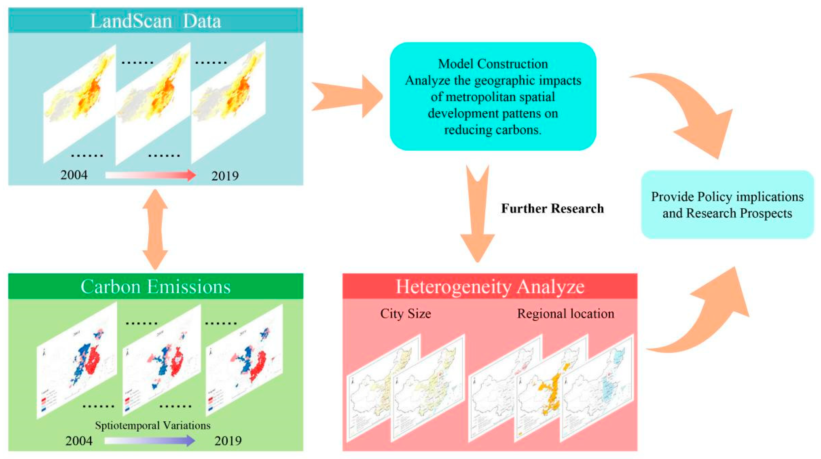
2. Methodology and Data

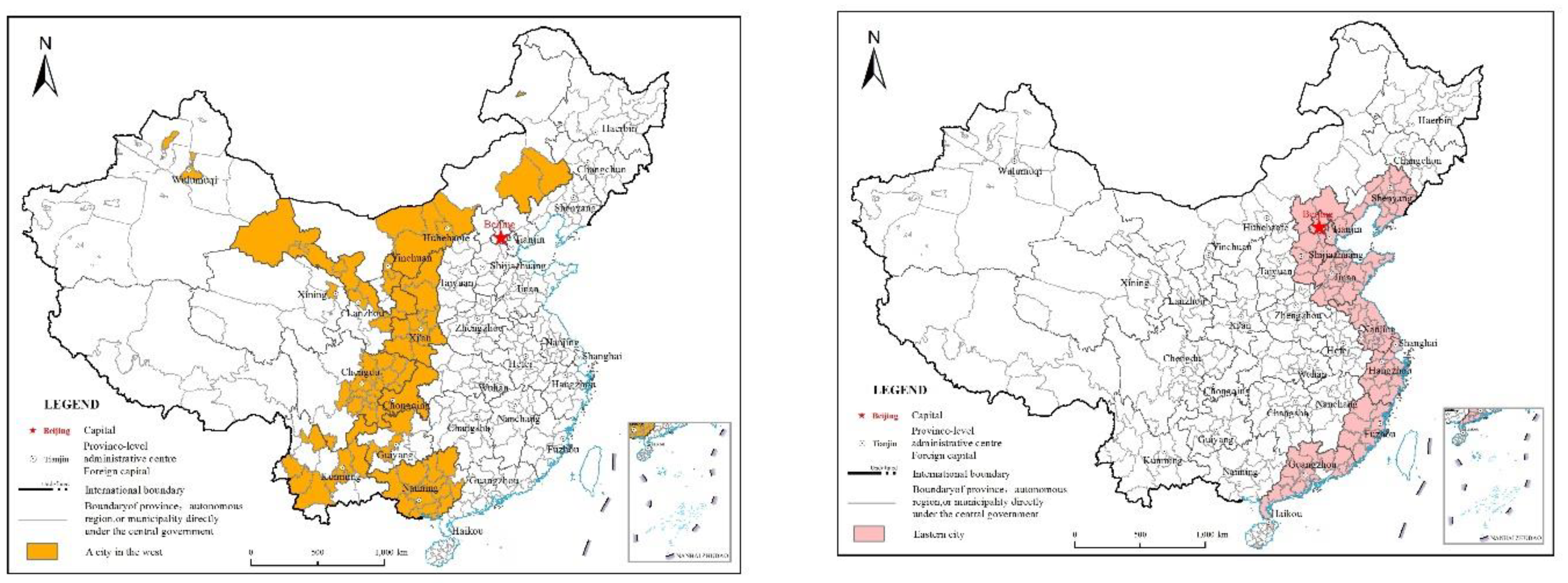
2.1. Study Area

This paper focuses on 278 cities at the prefecture level and above in mainland China (Figure 2), along with four cities under direct central control, i.e., Beijing, Tianjin, Shanghai, and Chongqing. In China’s administrative division system, prefecture-level cities are between provincial- and county-level units, and usually consist of a main urban area and many surrounding districts, county-level cities, counties, and subordinate units [45]. To some extent, prefecture-level cities are similar to intra-city spatial systems in that populations or economic activities can be clustered in core or peripheral areas.

2.2. Variables

2.2.1. Dependent Variable

Estimating carbon emissions (CE): Carbon emissions data are expressed by the CO₂ emissions per unit of gross regional product. Three types of energy methods are selected for measurement at the city level: liquefied petroleum, natural gas, and overall electricity generation [46]. Coal-based electricity demand is the main cause of CO₂ emissions; hence, coal-fired electricity generation is a more accurate measure of CO₂. Carbon emission factors for natural gas and LPG were set at 2.1622 kg/m³ and 3.1031 kg/kg, respectively, according to the Guidelines for the Preparation of Provincial Greenhouse Gas Inventories issued by the National Development and Reform Commission. The carbon emission factor for coal-fired power was set at 1.3023 kg/kWh, based on the uniform ratio for accounting in the China Electricity Yearbook of previous years.

2.2.2. Independent Variable

Coefficient of variation (COA): This study measures urban spatial development patterns based on the concept of ‘economic density proposed by Henderson [47], which constructs indicators to measure the distribution of average urban population density and intra-city population differentiation. Referring to the related literature, we construct a coefficient of variation term as an indicator of urban spatial development patterns [14], using LandScan data to identify urban centers through the spatial agglomeration of population density.

The coefficient of variation term was calculated by combining LandScan global population density distribution data with data from the Chinese Urban Statistical Yearbook. ArcGIS 10.2 software was used to extract the population density of each city from 2004 to 2019 from the boundaries of 278 prefecture-level cities, measured by raster pixel values. The population density of each extracted raster cell was divided by the total population of the city, and the result was multiplied by the population density per unit of raster. The results of these calculations were summed to obtain the economic density of the city, which is a measure of the average and internal population density of its agglomeration. The coefficient of variation term gives the ratio of the calculated economic density to the average population density of the city.

This research assumes two city types to understand the link between COV and urban spatial development trends. Cities 1 and 2 are compact and sprawling, respectively, with similar populations, urban areas, and density. City 1 and city 2 have the same population density on the center line, with 0 on the right and double on the left. Since they have the same average population density, city 2 has a coefficient of variation twice that of city 1. The coefficient of variation will be larger in cities with more population agglomeration. Therefore, the coefficient of variation term can reasonably characterize the spatial development pattern of a city.

2.2.3. Control Variables

To avoid the more serious omitted variable bias to strip out the impact of urban spatial development patterns on carbon emissions, this paper controls for relevant influences at the city level where possible. The control variables were selected in terms of economic development, financial growth, infrastructure development, and educational attainment [48,49]. Technological innovation (IA) captures the level of technology and capability of the economy and society [50]. Foreign openness (FI) describes the degree of transparency to the outside world and the impact of foreign investment on economic development [51]. Wage level (WAGE) represents the degree of high- or low-income workers [52], controlling for the impact of the above three variables on economic development. The level of financial development (FDL) is measured by year-end deposit and loan balances of financial institutions, and is a good indicator of the volume and convenience of financial size, effectively controlling the level of financial development [53]. The number of hospital beds (HOS) effectively controls the level of infrastructure development [54]. Human capital (HC) controls the educational attainment of society [55].

2.3. Data

For reasons of data availability, Hong Kong, Macau, and Taiwan are not included, and some cities with serious data deficiencies in the provinces of Tibet, Qinghai, Yunnan, Hainan, and others are excluded. Hence, the study included 278 prefecture-level cities across China from 2004 to 2019. All original data were obtained from spatial data from the LandScan Global Population Database, and statistical data were obtained from the China Statistical Yearbook, China Financial Yearbook, China Electricity Yearbook, China Energy Statistical Yearbook, and China Urban Statistical Yearbook.

Table 1. Description of variables in the models.

Variable	Definition	Computation Method	Data Source
lnCE	Carbon emission	Measurement of liquefied petroleum, natural gas, and community-wide electricity consumption at the city level	The World Bank World Development Indicators (WDI). http://data.worldbank.org/indicator (Accessed on 10 November 2022). China Electricity Yearbook China Energy Statistics Yearbook
lnCOV	Variation term	Extracted from LandScan Data using ArcGis 10.2	LandScan Global Population Database https://landscan.ornl.gov/ (Accessed on 10 November 2022)
lnIA	Innovation ability	Number of patent applications	China Urban Statistical Yearbook https:/stats.gov.cn/tjsj/ndsj/ (Accessed on 10 November 2022)
lnFI	Foreign investment	Total actual foreign capital used in the year/nominal GDP	China Urban Statistical Yearbook
lnWAGE	Wage level	Urban active workers income	China Urban Statistical Yearbook
lnHC	Human capital	Number of general undergraduates and above/city’s resident population	China Urban Statistical Yearbook China Statistical Yearbook
lnFDL	Financial development level	Financial institutions year-end deposit and loan balances	China Financial Yearbook
lnHOS	Hospital beds	Hospital beds per 10,000	China Urban Statistical Yearbook

shows the variables in the model. Natural logarithms were used for all variables to account for heteroscedasticity and regression model settings. To eliminate the influence of price rises, 2004 was chosen as the base year, and GDP of other years were deflated. Some missing values were interpolated linearly, as is common in statistical surveys [56], estimating missing information based on a linear pattern between known observations [57], saving processing time and non-response bias, and avoiding errors in the empirical analysis as much as possible [58].

2.4. Models

2.4.1. Spatial Weight Matrix Setting

To explore whether there is a spatial effect, we adopted Moran’s I index and constructs an economic–geographic weight matrix combining the economic and geographical characteristics of the urban development process,

$$\begin{array}{l}{W}_{ij}^e{=W}_{ij}^d\times diag(\overline{X_1}/\overline{X},\overline{X_2}/\overline{X},\dots \overline{X_n}/\overline{X})\\ W_{ij}^e=\left\{\begin{array}{l}\frac{W_{ij}^e}{{\displaystyle \sum W_{ij}^e}},i\ne j\\ 0,i=j\end{array}\right\}\end{array}$$

(1)

where W_ij is the matrix element in the i_th row and j_th column; d reflects the geographic distance, i.e., the economic distance spatial weight matrix, and is the average value of GDP per capital of each province and city j in the observation period, which is the average value of GDP per capital of all provinces and cities in the observation period. Standardized weights are noted as W.

2.4.2. Spatial Econometric Model

The Hausman test rejected the assumption of random effects in the model. The results are shown in

Table 2. Results of benchmark regression.

	(1)	(2)
Variables	Static SDM	Dynamic SDM
lnCEt-1		−0.342 ***
		(−4.013)
lnCOA	0.318 ***	0.374 *
	(4.871)	(1.891)
lnCOA2	−0.294 **	−0.116 **
	(−2.014)	(−2.043)
W.lnCOA	−0.412	0.348 *
	(−0.005)	(1.857)
W.lnCOA2	−0.436**	−0.296 ***
	(−2.118)	(−3.995)
lnIA	−0.041 ***	0.020 ***
	(−14.354)	(3.018)
lnFI	−0.084 ***	−0.015 ***
	(−3.985)	(−4.251)
lnWAGE	0.096 ***	0.091 ***
	(13.517)	(12.704)
lnHC	0.010	−0.004
	(0.000)	(−0.261)
lnFDL	0.006	−0.024
	(0.403)	(−0.389)
lnHOS	0.097 ***	−0.033 **
	(13.539)	(−2.231)
Time fixed effect	YES
Regional fixed effect	YES
Log L	126.978	107.856
N	4448	4448
R2	0.609	0.574
Hausman	123.62
	(0.013)

Note: *, **, and *** are significant at the statistical levels of 10%, 5%, and 1%, respectively. The same below.

, and the LM test is more suitable for this study than the surface spatial Durbin model. To mitigate the effects of heteroskedasticity, extreme values, and units of measure, a spatial Durbin model with dual fixed effects in time and space in logarithmic form is used for empirical purposes,

$$\begin{array}{ll}\ln C{E}_{it}=& \alpha {\displaystyle \sum _{j=1}^n{W}_{ij}\ln C{E}_{it}+{\epsilon }_1}{\displaystyle \sum _{j=1}^n{W}_{ij}\ln CO{A}_{it}+{\epsilon }_2{\displaystyle \sum _{j=1}^n{W}_{ij}(\ln CO{A}_{it}{)}^2}}+{\epsilon }_n{\displaystyle \sum _{j=1}^n{W}_{ij}\ln X_{it}}\\ \hspace{1em}& +{\eta }_1\ln CO{A}_{it}+{\eta }_2(\ln CO{A}_{it}{)}^2+{\eta }_n\ln X_{it}+{\mu }_i+{\kappa }_t+{\gamma }_{it}\end{array}$$

(2)

where CE denotes carbon emissions; COA denotes urban spatial development pattern; η₁, η₂, and η_n are regression coefficients; W_ij is the spatial weight matrix; X is the control variable; α is the spatial regression coefficient; ε is the spatial effect coefficient μ_i is the urban fixed effect; κ_t is the time fixed effect; and γ_it is the random error term.

Considering that there may be temporal inertia in urban spatial development patterns, we incorporates the previous urban spatial development patterns (COA) into the spatial Durbin model,

$$\begin{array}{ll}\ln C{E}_{it}=& \rho {\displaystyle \sum _{j=1}^n{W}_{ij}\ln C{E}_{it-1}+{\delta }_1}{\displaystyle \sum _{j=1}^n{W}_{ij}\ln CO{A}_{it}+{\delta }_2{\displaystyle \sum _{j=1}^n{W}_{ij}(\ln CO{A}_{it}{)}^2+{\delta }_n{\displaystyle \sum _{j=1}^n{W}_{ij}\ln X_{it}}}}\\ & +{\beta }_0+{\beta }_1\ln CO{A}_{it}+{\beta }_2(\ln CO{A}_{it}{)}^2+{\beta }_n\ln X_{it}+u_i+{\nu }_t+e_{it}\end{array}$$

(3)

where CE is carbon emissions; COA denotes urban spatial development pattern; β₀ is a constant term; β₁, β₂, and β_n denote the coefficients of the influencing factors; W_ij is the spatial weight matrix; X is the control variable; ρ is the spatial regression coefficient; δ is the spatial effect coefficient; υ_i is the urban fixed effect; ν_t is the time fixed effect; and e_it is the random error term.

3. Results and Discussion

3.1. Results of Spatial Econometric Model

3.1.1. Benchmark Regression

As shown in Table 2, the primary impact coefficient for VC is 0.318 and passes the 1% significance level, and the secondary impact coefficient is −0.294, passing the 5% significance level, indicating that compact urban spatial development has an inverted U-shaped effect on carbon emissions. In the early phases, every unit increase in urban compactness increases carbon emissions by 29.4% (Figure 3). This is likely due to increased traffic and population density in cities. Demand and energy usage raise carbon emissions. As the environment deteriorates and urban quality of life declines, the government takes measures such as regulating traffic, promoting new energy, having non-motorized vehicles on the roads, and greening the city to control carbon emissions, by increasing the compactness of urban spatial development patterns.

Technological innovation and foreign investment effects on carbon emissions are negative and pass the significance level test, while the effects of wage levels and infrastructure development on carbon emissions are positive and pass the significance level test. Financial development and human capital are positive but not significant, and may have a limited influence on carbon emissions; financial resource allocation and human capital supply should be optimized.

The regression coefficient of carbon emissions with a one-period lag is negative and significant at the 1% statistical level, indicating temporal inertia in carbon emissions and the scientific validity of adopting dynamic spatial measurement methods. As a result, in the long term, it is essential to pay attention to the impact of carbon emissions on the spatial dimension of urban spatial growth patterns.

3.1.2. The Decomposition Analysis

This work relates to the Lesage et al. study to investigate the geographical spillover effects of urban spatial development patterns on carbon emissions. The findings are divided into direct and indirect impacts.

Table 3. Results of decomposition analysis.

	Short-Term Effect		Long-Term Effect
	Direct Effect	Indirect Effect	Direct Effect	Indirect Effect
InCOA	0.354 ***	−0.115 ***	0.052	0.337 *
	(3.897)	(−3.882)	(1.026)	(1.889)
InCOA2	−0.268	0.214	−0.137 ***	0.235 ***
	(−0.034)	(0.548)	(−3.987)	(4.218)

shows how urban spatial growth patterns affect regional carbon emissions. The indirect impact is geographical spillover. In addition, this paper also decomposes the estimation results into short-term effects and long-term effects.

The decomposition results show that the direct effect on carbon emissions is a single positive effect in the short term, the impact coefficient 0.354, and it passes the significance test, for an inverted U-shaped effect in the long term. This may be due to the increase in local energy consumption caused by the compactness of urban space in the short term, but there is a gradual transformation of economic development towards green and high-quality development in the long term, which enhances energy recycling and reduces carbon emissions.

The indirect effect of urban spatial development patterns on carbon emissions has an impact factor of −0.115 in the short term, but a U-shape in the long term. This may be due to the siphoning effect formed by a larger population in the region in a shorter period, which relieves the pressure of energy demand in neighboring areas and reduces their carbon emissions in daily production. Over time, the large loss of people and resources from nearby areas causes a decrease in the economic and industrial structure of the neighboring districts, and manufacturing and heavy industries are developed to relieve economic strain. They also raise CO₂ emissions.

3.2. Robustness Checks

The first half of this study analyzes the baseline regression, followed by robustness tests by altering the explanatory factors, geographical weight matrix, and instrumental variables method.

3.2.1. Changing the Dependent Variable

Carbon intensity, or emissions per unit of carbon dioxide, is a comprehensive metric that integrates energy and industrial structure to assess carbon emissions, and has been used to validate the robustness of empirical data [59].

Table 4. Results of robustness check.

Variables	Change the Dependent Variable	Change the Spatial Weight Matrix	GS2SLS
L.lnCOAt-1			0.418 ***
			(3.579)
L.lnCOA2t-1			−0.175 **
			(−2.364)
lnCOA	−0.021 *	0.031 *
	(−1.852)	(1.783)
lnCOA2	−0.179 ***	−0.268 **
	(−3.974)	(−2.339)
W.lnCOA	0.049 **	0.084 **
	(2.512)	(2.071)
W.lnCOA2	−0.157 **	0.108 **
	(−2.413)	(2.015)
L.W.lnCOAt-1			0.146 ***
			(3.759)
L.W.lnCOA2t-1			0.237 ***
			(4.598)
Control variables	YES
Time fixed effect	YES
Regional fixed effect	YES
Cragg–Donald Wald F			243.579
Kleibergen–Paap rk Wald F			253.791
N	4448	4448	4448

Note: The YES means that the control variables are added to the regression model.

displays empirical results. The effect of the coefficient of variation on carbon intensity has an inverted U-shape, and the direction and strength of the control variables are generally consistent with previous work, thus, verifying the robustness of the baseline regression results.

3.2.2. Changing the Spatial Weight Matrix

This previous empirical study was based on a spatial Durbin model analysis using an economic and geographic weight matrix. A spatial weight matrix of geographic distances was created based on Euclidean distances to conduct a spatial econometric empirical analysis to confirm the robustness of the article’s benchmark regression results. The robustness test results are broadly similar to the prior study’s findings, as shown in Table 4.

3.2.3. Changing the Parameter Estimation Method

Generalized spatial two-stage least squares (GS2SLS) can effectively deal with the problems of model heteroskedasticity and endogeneity [60]. We employ GS2SLS to estimate the spatial econometric model’s parameters and chooses the explanatory variables and their multi-order as the instrumental variables for the explained variables’ spatial lags. Table 4 presents the empirical outcomes. It can be found that after the validity test of the explanatory variables lags by one period, it is found that the F-values are all greater than the critical value of Stock Yogo weak instrumental variables at 10%, indicating that there is no weak instrumental variable problem. At the same time, the rationality of the selected instrumental variables is verified. Urban development patterns have an inverted U-shaped influence on carbon emissions. The control variables mostly match the preceding section, confirming the baseline regression results.

3.3. Heterogeneity Analysis

Considering that urban spatial development patterns and carbon emission reduction may differ significantly across different spatial geographical locations, and that such differences may lead to biased estimates in the results of the overall or global empirical analysis, we prepared Moran scatter plots (Figure 4) and LISA plots (Figure 5) to explore whether spatial locational differences exist. Figure 4 shows that spatially, the vast majority of cities are in the first and third quadrants, high-high and low-low agglomeration types, indicating significant spatial aggregation in most cities. The Moran scatter plots for different years show that the spatial dependence of the distribution of urban spatial development patterns has remained relatively stable over the study period. Figure 5 depicts the spatial characteristics of heterogeneous carbon emissions using LISA maps, with high-high clusters concentrated in the eastern part of China, while low-low clusters are usually located in central, northeast, and southwest China. LISA maps for different years show that the spatial dependence of the distribution of carbon emissions has remained relatively stable over the study period. Figure 4 and Figure 5 show that spatial heterogeneity does exist. Therefore, in the reference literature, spatial heterogeneity is investigated from both city size and regional scale perspectives [61,62].

3.3.1. City Size Heterogeneity

To explore whether the dynamic relationship between the coefficient of variation term and carbon emissions varies by city size [63,64], we referred to studies measuring city sizes by year-end population and divided cities into large, medium, and small cities for heterogeneity analysis (Figure 6).

Table 5. Results of heterogeneity analysis based on city size.

Variables	Larger Cities	Small and Medium-Sized Cities
lnCOA	0.146 **	−0.307 *
	(2.413)	(−1.846)
lnCOA2	−0.121 *	−0.235
	(−1.903)	(−0.697)
W.lnCOA	0.185 ***	0.348 *
	(3.986)	(1.857)
W.lnCOA2	0.213 **	0.107
	(2.476)	(1.083)
Control variables	YES
Time fixed effect	YES
Regional fixed effect	YES
Log L	701.00	735.61
N	1840	2608
R2	0.462	0.773

Note: The YES means that the control variables are added to the regression model.

displays the outcomes.

In larger cities, a significant inverted U-shaped association is established between the primary coefficient of 0.416 and the quadratic coefficient of −0.121 for compact urban spatial development patterns and carbon emissions, which passes the significance level test. This shows that the pattern is initially not beneficial to lowering carbon emissions, and that the effect weakens with city size and vice versa in later phases. This may be because larger cities consume more energy in the early stages of development to promote economic growth and urban construction. Higher population concentrations lead to congestion effects, resulting in excessive carbon emissions. However, in the later years, the government takes measures to reduce carbon emissions, promotes the use of clean energy, and transforms the industrial structure, resulting in significant carbon emission reduction.

The primary and secondary coefficients of the spatial effect are positive, they pass the significance test, and the effect on carbon emissions from neighboring areas is U-shaped. This shows that compact city expansion is not favorable to carbon reduction in nearby areas in the early phases, but later it is. This may be because early bigger cities were more spatially constrained, leading to a deterioration in the local biological environment, quality of life, and production. Many people flow to nearby areas, resulting in a modest carbon emission reduction. Later, the siphon effect generated by improving ecological buildings and developing new regional sectors leads to the repatriation of talents from nearby regions, reducing carbon emissions in neighboring areas.

The principal coefficient of variation in carbon emissions in small and medium-sized cities is −0.307, and it is significant, while the second-term coefficient is not significant. This suggests that the spatial development pattern of compact cities is conducive to reducing carbon emissions, and that the smaller the city, the more significant the reduction. The spatial concentration of the urban population is relatively low in small or medium-sized cities, and the concentration effect is exerted through a compact population distribution. This produces larger environmental advantages within the city.

The spatial effect coefficient is 0.348, which indicates that the spatial development pattern of compact cities in the region has a positive impact on the carbon reduction in neighboring areas. This may be because the region’s small and medium-sized cities have a high population density, which promotes economic growth and labor demand. Some people from adjacent areas may come to the region for work, which shifts their industrial structure to high-tech companies and reduces carbon emissions. Therefore, small and medium-sized cities should adopt a compact urban spatial development strategy, whereas bigger cities should slow down the pace to reduce carbon emissions.

3.3.2. Regional Location Heterogeneity

To explore whether the impact of urban spatial development patterns on carbon emissions varies due to regional heterogeneity, this paper’s data were divided into eastern, central, and western regions for heterogeneity analysis (Figure 7), the results of which are shown in

Table 6. Regional-level empirical results.

Variables	Eastern Region	Central Region	Western Region
lnCOA	0.214 *	0.223 **	−0.361 ***
	(1.869)	(2.305)	(−3.978)
lnCOA2	−0.325 **	−0.351	0.348
	(−2.436)	(-0.023)	(0.299)
W.lnCOA	0.371 **	0.348 *	0.014
	(2.397)	(1.857)	(1.015)
W.lnCOA2	0.193 **	0.237	0.097
	(2.308)	(1.095)	(0.078)
Control variables	YES
Time fixed effect	YES
Regional fixed effect	YES
Log L	377.65	426.52	507.71
N	1584	1600	1264
R2	0.438	0.180	0.394

Note: The YES means that the control variables are added to the regression model.

.

The coefficient of variation term for the eastern region has a negative quadratic coefficient of influence on carbon emissions and passes the significance test at the 5% level, showing an inverted U-shaped relationship. The spatial development pattern of compact cities does not help lower carbon emissions in the early stages, but it does when population density grows, perhaps because the east is a developed metropolis with a significant influx of people to solve the job troubles. Population density causes environmental degradation. With deepening economic reform, the eastern region’s industrial structure is converting into high-tech businesses that require less labor and lower carbon emissions. The quadratic coefficient of the spatial effect is positive in a U-shape, indicating that the spatial growth pattern of compact cities in the region is not beneficial to carbon emission reduction in nearby regions in the early stage but is in the later stage.

The central region’s coefficient of variation positively influences carbon emissions, the impact factor is 0.223, indicating that compact spatial development increases carbon emissions. This may be because the central region consists primarily of industrial cities, which consume more natural resources and energy, increasing carbon emissions. The spatial effect influence coefficient is 0.348; the more compact the spatial development pattern of cities in the region, indicating that it leads to an increase in carbon emissions from neighboring places, perhaps because the local area attracts more population clusters for economic development, leading neighboring places to learn from local production and business practices to form economies of scale for economic growth.

The coefficient of variation term for the western region has an impact factor of −0.361 on carbon emissions, indicating that compact cities will reduce carbon emissions, because of the relatively backward development of western urban cities. National policies focus on urban planning and construction in the west, emphasizing the protection of ecological civilization and the regional diversification of urban sector development, which can reduce urban residents’ energy consumption.

3.4. Discussion

Our findings provide a basis for reducing carbon emissions from the perspective of urban spatial development patterns and can lead to the following policy recommendations. First, the sprawl of the urban population will drive up carbon emissions, and there is a need to prevent over-dispersal of the population in the process of urban development and to further strengthen the clustering of the urban population around central areas. Second, small and medium-sized cities should adopt a compact spatial development plan based on their dense public transport networks to avoid excessive population concentration. Third, with the adoption of a compact urban spatial development model, supporting facilities for population concentration should be established, such as efficient urban road networks and energy transportation pipelines, to achieve more environmentally friendly and efficient emission-reduction goals.

Although the effects of urban spatial development patterns on carbon emission reduction have been initially investigated, some limitations warrant further study. For example, we measured urban spatial development patterns from the level of urban population density, which is still not very comprehensive, although it complements past studies. In addition, the research object of this paper is based on the Chinese context, and other countries and economies must still be explored.

References

1. Zhao, B.; Sun, L.; Qin, L. Optimization of China’s provincial carbon emission transfer structure under the dual constraints of economic development and emission reduction goals. Environ. Sci. Pollut. Res. 2022, 83, 110–120. [Google Scholar] [CrossRef] [PubMed]
2. Jalil, A.; Mahmud, S.F. Environment Kuznets curve for CO2 emissions: A cointegration analysis for China. Energy Policy 2009, 37, 5167–5172. [Google Scholar] [CrossRef] [Green Version]
3. Daskalakis, G. Temporal restrictions on emissions trading and the implications for the carbon futures market: Lessons from the EU emissions trading scheme. Energy Policy 2020, 115, 88–91. [Google Scholar] [CrossRef] [Green Version]
4. Li, Y.; Derudder, B. Dynamics in the polycentric development of Chinese cities, 2001–2016. Urban Geogr. 2020, 56, 272–292. [Google Scholar] [CrossRef]
5. Cortinovis, N.; Vanort, F.G. Between spilling over and boiling down: Network-mediated spillovers, absorptive capacity and productivity in European regions. J. Econ. Geogr. 2019, 19, 1233–1260. [Google Scholar] [CrossRef] [Green Version]
6. Burger, M.; Meijers, E. Form follows function? Linking morphological and functional Polycentricity. Urban Stud. 2012, 49, 1127–1149. [Google Scholar] [CrossRef]
7. Veneri, P.; Burgalassi, D. Questioning polycentric development and its effects. Issues of definition and measurement for the Italian NUTS-2 regions. Eur. Plan. Stud. 2012, 20, 1017–1037. [Google Scholar] [CrossRef] [Green Version]
8. Peris, A.; Meijers, E.; Ham, M. The evolution of the system of cities literature since 1995: Schools of thought and their interaction. Netw. Spat. Econ. 2019, 18, 533–554. [Google Scholar] [CrossRef] [Green Version]
9. Münter, A.; Volgmann, K. Polycentric regions: Proposals for a new typology and terminology. Urban Stud. 2020, 37, 1983–1997. [Google Scholar] [CrossRef]
10. Zeng, C.; Zhou, Y.; Wang, S.; Yan, F.; Zhao, Q. Population spatialization in China based on night-time imagery and land use data. Int. J. Remote Sens. 2011, 32, 9599–9620. [Google Scholar] [CrossRef]
11. Zhuo, L.; Ichinose, T.; Zheng, J.; Chen, J.; Shi, P.J.; Li, X. Modelling the population density of China at the pixel level based on DMSP/OLS non-radiance-calibrated night-time light images. Int. J. Remote Sens. 2009, 30, 1003–1018. [Google Scholar] [CrossRef]
12. Gaughan, A.E.; Stevens, F.R.; Huang, Z.; Nieves, J.J.; Sorichetta, A.; Lai, S.; Ye, X.; Linard, C.; Hornby, G.M.; Hay, S.I.; et al. Spatiotemporal patterns of population in mainland China, 1990 to 2010. Sci. Data 2016, 3, 160005. [Google Scholar] [CrossRef] [PubMed] [Green Version]
13. Schneider, A.; Mertes, C.M.; Tatem, A.J.; Tan, B.; Sulla-Menashe, D.; Graves, S.J.; Patel, N.N.; Horton, J.A.; Gaughan, A.E.; Rollo, J.T. A new urban landscape in East–Southeast Asia, 2000–2010. Environ. Res. Lett. 2015, 10, 034002. [Google Scholar] [CrossRef]
14. Liu, X.; Li, S.; Qin, M. Urban spatial structure and regional economic efficiency--and the model choice of China’s urbanization development path. Manag. World 2017, 1, 51–64. [Google Scholar] [CrossRef]
15. Gilles, D.; Matthew, A. Urban form and driving: Evidence from US cities. J. Urban Econ. 2018, 108, 170–191. [Google Scholar] [CrossRef]
16. Thinh, N.X.; Arlt, G.; Heber, B.; Hennersdorf, J.; Lehmann, I. Evaluation of urban land-use structures with a view to sustainable development. Environ. Impact Assess. Rev. 2002, 22, 475–492. [Google Scholar] [CrossRef]
17. Ye, C.; Sun, C.; Chen, L. New evidence for the impact of financial agglomeration on urbanization from a spatial econometrics analysis. J. Clean. Prod. 2018, 200, 65–73. [Google Scholar] [CrossRef]
18. Lu, S.; Shi, C.; Yang, X. Impacts of Built Environment on Urban Vitality: Regression Analyses of Beijing and Chengdu, China. Int. J. Environ. Res. Public Health 2019, 16, 4592. [Google Scholar] [CrossRef] [Green Version]
19. Edward, L.; Glaeser, T. Chapter 56—Sprawl and Urban Growth. Handb. Reg. Urban Econ. 2004, 4, 2481–2527. [Google Scholar] [CrossRef]
20. Cheng, K.; Li, J. Empirical evidence of compact cities and sustainable development in China. Financ. Econ. Res. 2007, 10, 73–82,106. [Google Scholar] [CrossRef]
21. Wang, W.; Zhang, Y. Financial structure, industrial structure upgrading and economic growth—A perspective of technological progress based on different characteristics. Econ. 2022, 2, 118–128. [Google Scholar] [CrossRef]
22. Hamidi, S.; Zandiatashbar, A. Does urban form matter for innovation productivity? A national multi-level study of the association between neighbourhood innovation capacity and urban sprawl. Urban Stud. 2019, 56, 1576–1594. [Google Scholar] [CrossRef]
23. Kim, J.; Brownstone, D. The impact of residential density on vehicle usage and fuel consumption. Acad. Press 2009, 65, 95–98. [Google Scholar] [CrossRef] [Green Version]
24. Chen, H.; Jia, B. Sustainable urban form for Chinese compact cities: Challenges of a rapid urbanized economy. Habitat Int. 2007, 32, 28–40. [Google Scholar] [CrossRef]
25. Yang, L.; Li, Z. Technology advance and the carbon dioxide emission in China—Empirical research based on the rebound effect. Energy Policy 2017, 101, 150–161. [Google Scholar] [CrossRef]
26. Shao, S.; Zhao, K.; Dou, J. Energy saving and emission reduction effects of economic agglomeration:theory and Chinese experience. Manag. World 2019, 35, 36–60,226. [Google Scholar] [CrossRef]
27. Zhang, K.; Wang, D. Interactive effects of economic agglomeration and environmental pollution and spatial spillover. China Ind. Econ. 2014, 6, 70–82. [Google Scholar] [CrossRef]
28. Roca, J.; Alcántara, V. Energy intensity, CO2 emissions and the environmental Kuznets curve. The Spanish case. Energy Policy 2001, 29, 553–556. [Google Scholar] [CrossRef]
29. Zhao, H.; Wang, B.; Liu, T. Empirical analysis on the factors influencing national and regional carbon intensity in China. Renew. Sustain. Energy Rev. 2016, 55, 34–42. [Google Scholar] [CrossRef]
30. Poumanyvong, P.; Kaneko, S. Does urbanization lead to less energy use and lower CO2 emissions? A cross-country analysis. Ecol. Econ. 2010, 70, 434–444. [Google Scholar] [CrossRef]
31. Martínez-Zarzoso, I.; Maruotti, A. The impact of urbanization on CO2 emissions: Evidence from developing countries. Ecol. Econ. 2011, 70, 1344–1353. [Google Scholar] [CrossRef] [Green Version]
32. Chen, Y.; Sun, Y.X.; Wang, X.J. Research on the impact of global scientific and technological innovation on carbon productivity and countermeasures. China Popul. Resour. Environ. 2019, 29, 30–40. [Google Scholar]
33. Sher, V.K.; Wing, I.S. Accounting for quality: Issues with modeling the impact of R&D on economic growth and carbon emissions in developing economies. Energy Econ. 2008, 30, 2771–2784. [Google Scholar] [CrossRef]
34. Kerui, D.; Li, P. Do green technology innovations contribute to carbon dioxide emission reduction? Empirical evidence from patent data. Technol. Forecast. Soc. Change 2019, 146, 297–303. [Google Scholar] [CrossRef]
35. Beck, N.; Katz, J.N. What To Do (and Not to Do) with Time-Series Cross-Section Data. Am. Political Sci. Rev. 1995, 89, 634–647. [Google Scholar] [CrossRef]
36. Guo, J.H.; Li, B.Y. Evolutionary game analysis of duopoly’s remanufacturing entry decision. Syst. Eng. Theory Pract. 2013, 33, 370–377. [Google Scholar]
37. Christophers, B. Mind the rent gap: Blackstone, housing investment and the reordering of urban rent surfaces. Urban Stud. 2022, 59, 698–716. [Google Scholar] [CrossRef]
38. He, W.; Zhang, H.; Chen, X.; Yan, J. An empirical study on population density, industrial agglomeration and carbon emissions in Chinese provinces-based on the perspective of agglomeration economy, congestion effect and spatial effect. Nankai Econ. Res. 2019, 2, 207–225. [Google Scholar] [CrossRef]
39. Tang, L.; Hu, Z.; Su, J.; Xiao, P. Threshold characteristics and regional differences in the impact of urbanization on domestic carbon emissions. J. Manag. 2015, 12, 291–298. [Google Scholar] [CrossRef]
40. Li, Y.; Liu, X. How did urban polycentricity and dispersion affect economic productivity? A case study of 306 Chinese cities. Landsc. Urban Plan. 2018, 173, 51–59. [Google Scholar] [CrossRef]
41. Zhang, K.; Zhang, J. Urban cluster polycentricity and green development efficiency--an analysis of the spatial layout of urbanization based on heterogeneity. China Popul. -Resour. Environ. 2022, 32, 107–117. [Google Scholar] [CrossRef]
42. Han, F.; Xie, R.; Iu, Y.; Fang, J.; Liu, Y. The effects of urban agglomeration economies on carbon emissions: Evidence from Chinese cities. J. Clean. Prod. 2018, 172, 1096–1110. [Google Scholar] [CrossRef]
43. Azka, A.; Waqar, A.; Hazrat, Y.; Akbar, M. Financial Development, Institutional Quality, and the Influence of Various Environmental Factors on Carbon Dioxide Emissions: Exploring the Nexus in China. Front. Environ. Sci. 2022, 9, 121–130. [Google Scholar] [CrossRef]
44. Desmet, K.; Gomes, J.; Ortuño, I. The geography of linguistic diversity and the provision of public goods. J. Dev. Econ. 2020, 143, 102384. [Google Scholar] [CrossRef] [Green Version]
45. Wang, Y.; Wang, C.; Hong, J.; Nian, M. Natural conditions, administrative hierarchy and urban development in China. Manag. World 2015, 1, 41–50. [Google Scholar] [CrossRef]
46. Ren, X.S.; Liu, Y.J.; Zhao, G.H. Impact of economic agglomeration on carbon emission intensity and transmission mechanism. China Popul.-Resour. Environ. 2020, 30, 95–106. [Google Scholar]
47. Hansen, B.E. Threshold Effects in Non-Dynamic Panels: Estimation, Testing and Inference. J. Econom. 1999, 93, 345–368. [Google Scholar] [CrossRef] [Green Version]
48. Walker, H.W.; Antonio, M. Agglomeration: A long-run panel data approach. J. Urban Econ. 2017, 99, 1–14. [Google Scholar] [CrossRef] [Green Version]
49. Giovanni, M.; Marianna, M. The Impact of the European Emission Trading Scheme on Multiple Measures of Economic Performance. Environ. Resour. Econ. 2018, 71, 551–582. [Google Scholar] [CrossRef]
50. Baptist, S.; Teal, F. Technology and Productivity in African Manufacturing Firms. World Dev. 2014, 64, 713–725. [Google Scholar] [CrossRef]
51. Lee, J. The contribution of foreign direct investment to clean energy use, carbon emissions and economic growth. Energy Policy 2013, 55, 483–489. [Google Scholar] [CrossRef]
52. Ye, J.Y.; Wu, L.W. Social capital and the wage level of migrant workers—Resource measurement and causal identification. Economics 2014, 13, 1303–1322. [Google Scholar] [CrossRef]
53. Wang, M.; Zhou, J.; Long, Y. Outside the ivory tower: Visualizing university students’ top transit-trip destinations and popular corridors. Reg. Stud. 2016, 3, 202–206. [Google Scholar] [CrossRef]
54. Rouse, P.; Wodenitscharow, K. Equity and Health Inequalities: Should DCEA be Considered for Decision Making in the United Kingdom? Value Health 2022, 25, S86. [Google Scholar] [CrossRef]
55. Park, J. International and Intersectoral R&D Spillovers in the OECD and East Asian Economies. Econ. Inq. 2004, 42, 739–757. [Google Scholar] [CrossRef]
56. Yang, J.; Yu, Z.; Ding, W. Interpolation methods for missing data in sample surveys. Math. Stat. Manag. 2008, 5, 821–832. [Google Scholar] [CrossRef]
57. Liu, Z.; Yau, C. A propensity score adjustment method for longitudinal time series models under nonignorable nonresponse. Stat. Pap. 2021, 18, 317–342. [Google Scholar] [CrossRef]
58. Lu, G.; Copas, J.B. Missing at Random, Likelihood Ignorability and Model Completeness. Ann. Stat. 2004, 32, 754–765. [Google Scholar] [CrossRef] [Green Version]
59. Shao, S.; Fan, M.; Yang, L. Economic restructuring, green technological progress and low-carbon transformational development in China-an empirical examination based on the perspective of overall technological frontier and spatial spillover effects. Manag. World 2022, 38, 46–69+4-10. [Google Scholar] [CrossRef]
60. Kelejian, H.H.; Ingmar, R. A Generalized Spatial Two-Stage Least Squares Procedure for Estimating a Spatial Autoregressive Model with Autoregressive Disturbances. J. Real Estate Financ. Econ. 1998, 17, 99–121. [Google Scholar] [CrossRef]
61. Yu, B. Can agglomeration of productive service industries improve manufacturing productivity? An analysis based on industry, regional and city heterogeneity perspectives. Nankai Econ. Res. 2017, 2, 112–132. [Google Scholar] [CrossRef]
62. Sharif, H.M. Panel estimation for CO2 emissions, energy consumption, economic growth, trade openness and urbanization of newly industrialized countries. Energy Policy 2011, 39, 6991–6999. [Google Scholar] [CrossRef]
63. Meijers, E. Summing small cities does not make a large city: Polycentric urban regions and the provision of cultural, leisure and sports amenities. Urban Stud. 2018, 45, 2323–2342. [Google Scholar] [CrossRef]
64. Haider, H.; Hewage, K.; Umer, A.; Ruparathna, R. Sustainability Assessment Framework for Small-sized Urban Neighbourhoods: An Application of Fuzzy Synthetic Evaluation. Sustain. Cities Soc. 2017, 12, 21–32. [Google Scholar] [CrossRef]
Figure 1. The flow chart of this paper.
Land 11 02031 g001
Figure 2. Location map of China.
Land 11 02031 g002
Figure 3. Coefficient of variation shape.
Land 11 02031 g003
Figure 4. Scatterplots of the degree of COA and dispersion in 2004, 2009, 2014, and 2019.
Land 11 02031 g004
Figure 5. LISA maps of carbon emission distribution, 2004–2019.
Land 11 02031 g005
Figure 6. Distribution of small, medium, and large cities.
Land 11 02031 g006
Figure 7. East, central, and west city distribution.
Land 11 02031 g007aLand 11 02031 g007b