Abstract
The knowledge about the spatial distribution of soil organic carbon stock (SOCS) helps in sustainable land-use management and ecosystem functioning. No such study has been attempted in the complex topography and land use of Himalayas, which is associated with great spatial heterogeneity and uncertainties. Therefore, in this study digital soil mapping (DSM) was used to predict and evaluate the spatial distribution of SOCS using advanced geostatistical methods and a machine learning algorithm in the Himalayan region of Jammu and Kashmir, India. Eighty-three soil samples were collected across different land uses. Auxiliary variables (spectral indices and topographic parameters) derived from satellite data were used as predictors. Geostatistical methods—ordinary kriging (OK) and regression kriging (RK)—and a machine learning method—random forest (RF)—were used for assessing the spatial distribution and variability of SOCS with inter-comparison of models for their prediction performance. The best fit model validation criteria used were coefficient of determination (R2) and root mean square error (RMSE) with resulting maps validated by cross-validation. The SOCS concentration varied from 1.12 Mg/ha to 70.60 Mg/ha. The semivariogram analysis of OK and RK indicated moderate spatial dependence. RF (RMSE = 8.21) performed better than OK (RMSE = 15.60) and RK (RMSE = 17.73) while OK performed better than RK. Therefore, it may be concluded that RF provides better estimation and spatial variability of SOCS; however, further selection and choice of auxiliary variables and higher soil sampling density could improve the accuracy of RK prediction.
1. Introduction
The presence of an adequate amount of organic carbon in soil has a substantial effect on the improvement of soil health. It ameliorates soil physical properties such as structure, nutrient cycles, and water holding capacity, etc. [1,2,3,4]. However, various factors such as climate, relief, vegetation type, and land use affect its spatial distribution [5,6,7]. Moreover, the carbon dioxide fluxes occurring between the atmosphere and soil system are responsible for the changes in SOC stocks [8,9]. Therefore, its accurate estimation matters in managing global environmental issues and food security [10,11,12]. However, the distribution of soil organic carbon is uneven over the earth’s surface, affected by various factors such as topography, parent materials, climate, and biological activities [13]. Considering that the nature of these factors is different for different places, it becomes difficult to develop a single method that can determine the complex distribution of SOCS over the landscape [14]. However, with time many geologists and soil scientists have developed advanced geostatistical and machine learning algorithms that could remove the uncertainties to a fair extent and provide more accurate mapping techniques [15,16,17].
Digital maps of soil properties can be prepared from finite location samples using geostatistical methods [18]. It can capture the continuous nature of the properties of soil and random differences during modeling that depend upon their spatial correlation over the landscape [19]. Many geostatistical models, such as ordinary kriging, regression kriging, linear regression, cokriging, and inverse distance weighted regression, etc., have been used in soil mapping owing to their capability of accurate prediction and error minimization [20]. Moreover, machine learning algorithms such as regression tree, support vector regression, cubist, and random forest, among others, developed over the past years correlate environment variables with the soil properties and capture nonlinear relationships, leading to better prediction and accurate results [17,21,22]. Many authors have used these environmental or auxiliary variables, such as vegetation indices, and topographical attributes to build a spatial model for mapping soil properties [6,23,24]. These auxiliary variables could be extracted from various sources such as remote sensing and digital elevation models, etc. [25,26].
The surge in acceptance and application of these mapping techniques is because of the availability of huge databases including the data of inferred or measured soil properties, extracted auxiliary variables, and the numeric model development that can work on this huge amount of data [27]. The use of geostatistical and machine learning algorithms in soil science has transformed the way of generating soil maps [28]. These algorithms are based on the quantitative relationship between soil and the auxiliary covariates for soil property prediction to overcome the limitations of the conventional methods used. However, the inter-model comparison studies in DSM for different soil properties reveal differential applications based on uncertainty and prediction accuracy [29,30,31,32] for situation-specific advantages and disadvantages of the models [33]. Keeping this in mind, the study was conducted to predict SOCS at 30 m resolution of the complex topography of the Wangath watershed of Ganderbal district using geostatistical methods, viz., ordinary kriging (OK) and regression kriging (RK), and machine learning method, viz., random forest (RF), and comparing their performance for prediction accuracy.
2. Materials and Methods
2.1. Study Area
The current study was conducted for the Wangath watershed located in the Western Himalayas between 34°27′ and 34°46′ N and 74°88′ and 75°09′ E of Ganderbal district of Jammu and Kashmir UT of India (Figure 1). The area falls under the temperate agroclimatic zone with an average annual rainfall of 676 mm and temperature ranging from 3.9 to 22.56 °C. The watershed is located in the Sindh catchment, spread over an area of 30,980 ha with a perimeter of 95 km. The watershed has an elevation of about 2000 to 4500 m above mean sea level, and the area is under different land uses, viz., apple, maize, paddy, forest, and wasteland. The slope of the area varies from 0 to 60%. The hilly area is dominated by the species of Pinus sylvestris, Pinus walichiana, Cedrus deodara, Abies pindrow, and Piceasmitheana. The soil texture is dominated by clay loam and silty clay loam.
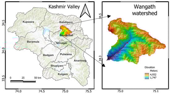
Figure 1.
Wangath watershed study area with sampling points.
2.2. Soil Sampling and Analysis
The eighty-three surface soil samples at 0–30 cm depth were collected using the purposive soil sampling method in highly difficult terrain in a 1.5 × 1.5 km unregular grid sampling design. The GPS (global positioning system) receiver was used to record the latitude and longitude of the area. The soil samples were processed and analyzed by Walkley and Black method for soil organic carbon estimation [34]. Core samples were used for determining the bulk density [35].
2.3. SOC Stock Estimation
SOC stocks were derived from the amount of organic carbon through the below-mentioned Equation:
where SOCS is soil organic carbon stocks of all the soil sections taken (Mg ha−1), SOC represents the SOC content (g kg−1), ρb implies bulk density (Mg m−3), d represents thickness (cm) of the layers, and δ is the percentage of course fragments (>2 mm) [36].
2.4. Auxiliary Covariates
In this study, the auxiliary variables such as satellite spectral indices and topographical attributes were extracted from Landsat 8 (OLI and TIRS) and SRTM DEM, respectively. The Landsat data acquired on 22 June 2020 from USGS (United States Geological Survey) Earth Explorer were used to extract thirteen satellite spectral indices (Table 1), viz., brightness index (BI), wetness index (WI), vegetation condition index (VCI), greenness index (GI), normalized difference vegetation index (NDVI), ratio vegetation index (RVI), perpendicular vegetation index (PVI), and soil-adjusted vegetation index (SAVI), etc. Meanwhile, the topographical factors (Table 1) of primary and secondary terrain variables—viz., slope, elevation, aspect, profile curvature, flow direction, topographic position index (TPI), SAGA wetness index (SWI), compound topographic index (CTI), total upslope length (TUL), longest upslope length (LUL), and stream power index (SPI)—were obtained from the SRTM DEM downloaded from USGS Earth Explorer (https://earthexplorer.usgs.gov). Moreover, the geometric correction and projection of the Landsat image were conducted from WGS 84 into a UTM Zone 43N coordinate system. The watershed delineation and image processing of the selected area were carried out in QGIS 3.18.

Table 1.
Auxiliary covariates derived from the satellite data.
2.5. Geostatistical and Machine Learning Techniques
2.5.1. Ordinary Kriging
Ordinary kriging (OK) is a geostatistical technique that uses interpolation to estimate the value at an unsampled location by utilizing the neighboring known data [56,57]. OK is a multipart process where a variogram is fitted to the input data determining the spatial variance structure of the observed values that help in assessing kriging weights for interpolation of unsampled locations across the spatial field. OK exploits the spatial autocorrelation of the observed points to interpolate the values in the spatial field with distance as a function defined by the variogram modeling. The spatial dependence of SOCS was evaluated through experimental semivariogram modeling. Kriging weights are generally calculated based on the distance between observed values and the target location; the closer the observed points are to the point of interest, the more weight it gains [58]. It assumes the concept of stationarity, which means that the mean and variance are constant across the spatial field. It uses the below-mentioned Formula:
where is the estimated value at the unsampled point , is the measured value at , is the weighting coefficient, and n is the number of points considered in the searching domain.
2.5.2. Regression Kriging
Regression kriging is a combination of two methods, viz., regression and kriging where regression is applied to fit the variation of auxiliary variables with soil properties, and the simple kriging with an expected value of 0 is applied to fit the residuals, i.e., unexplained variation [59]. In simple terms, it is a spatial prediction technique involving two aspects; the first is the regression of dependent or target variables with the explanatory or auxiliary variables such as topographic attributes and remote sensing indices, etc., and the second is the kriging of residuals. Regression kriging is based on certain assumptions, viz; linearity, normality, collinearity, and homoscedasticity. The description of regression kriging is demonstrated below:
where is the interpolated value at , gives the fitted drift, is the interpolated residual, stands for the estimated drift model coefficients ( is the estimated intercept), represents the kriging weights resolved by the spatial dependence structure of the residual, and is residual at .
2.5.3. Random Forest
Random forest (RF) is a recursive partitioning method that grows several regression trees and averages the results [60]. The classification or regression trees are calculated on random subsets of data (bootstrap samples) using randomized predictor variables at each tree. The result of numerous trees grown within the algorithm is averaged to give out a single prediction. Random forest comes under the supervised learning method, which refers to the training of algorithms using labeled datasets so that the model can map the outcome of the new dataset accurately. In simple terms, a random forest is a classification algorithm that utilizes randomness in selecting the predictor variables for building individual trees, thereby trying to build an uncorrelated forest of trees. The results of all the made trees are merged to attain a more accurate and reliable prediction. The description is given by:
where b is the individual bootstrap sample, B is the total number of trees, and t*b _b is the individual decision tree.
The soil samples were randomly split into training (75%) and validation (25%) sets, and a cross-validation strategy (10-fold or k = 10) was implemented in the train function to select the best hyperparameters, viz., ntree and mtry. As k of either 5 or 10 reduces the biasness of the estimate [61], the mtry parameter controls the number of covariates randomly used at each split, and ntree controls the number of trees generated by random forest. The out-of-bag RMSE was used to select the best mtry model. The number of trees was plotted against out-of-bag RMSE to analyze ntree parameters, and the best ntree (ntree = 600) was selected when the relationship stabilized at the minimum possible RMSE. The default setting for covariate reduction was mtry = p/3. By iterating through mtry = 1, 2, …, p, we were able to determine the best mtry for the final set of covariates by minimizing out-of-bag RMSE. Figure 2 represents the flowchart of the methodology adopted.
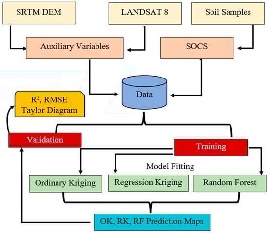
Figure 2.
Flow chart of the methodology adopted.
2.6. Model Validation
The selected models were assessed using the criteria of coefficient of determination (R2) and root mean square error (RMSE) as per the following Equations:
where Pi is the predicted and Oi denotes measured values at the ith point, Oavg, Pavgis the average of measured and predicted soil property values at the ith point, and “n” denotes total no. of data points, and “p” denotes the number of predictors used. The difference between measured and predicted values of soil properties at the validation locations determines the root mean square error. The small values of RMSE and high R2 determine the accurate prediction model. This was in accordance with the standard set by Li et al. [2] for R2 values: <0.50 (unacceptable prediction), <0.75 (acceptable prediction), and >0.75 (good prediction). The result validation was also supplemented by a Taylor diagram, which describes three aspects, viz., Pearson’s correlation coefficient, RMSE, and standard deviation [62]. All descriptive statistics, and geostatistical methods—OK, RK, and random forest—were computed using R software 3.6.1 [63].
3. Results and Discussion
3.1. Statistical Analysis of SOC Stocks
The statistical parameters of SOCS—viz., mean, min, and max; 95% confidence interval; maximum difference rate (MDR); coefficient of variation (CV); and standard deviation—are shown in Table 2. The SOCS concentration varied from 1.12 Mg/ha to 70.60 Mg/ha. The percentage of the coefficient of variation of SOCS was 33.81, and the average SOCS of the study area was 26.48 Mg/ha. The higher value of CV is attributed to the effect of environmental factors and measurement errors [64].
Table 2.
Descriptive statistics.
SOCS followed the trend of horticulture > paddy > forestry > maize > wasteland, with mean values of 46.26, 33.01, 30.23, 13.12, 5.48 Mg/ha, respectively (Table 3). This suggests that the soil properties are significantly affected by different land uses; as revealed by Wan et al. [65], there is a nexus between soil property and the management strategies exemplified by the quantity and frequency of the fertilizer applied. Similar findings were reported by Liu et al. [66] and Bangroo et al. [6] that among the other environmental factors, land-use types strongly affect soil organic carbon distribution.
Table 3.
SOC stocks under different land uses.
3.2. Correlation of SOCS with Environmental Variables
The study showed SOCS positively and significantly correlated (Table 4) with the wetness index (r = 0.41, p < 0.01), vegetation condition index (r = 0.32, p < 0.01), normalized difference vegetation index (r = 0.30, p < 0.01), ratio vegetation index (r = 0.31, p < 0.01), soil-adjusted vegetation index (r = 0.30, p < 0.01), clay index (r = 0.27, p < 0.05), and hue index (r = 0.23, p < 0.05), which could be attributed to wetter climates at higher topographic positions with more vegetation. The results are in corroboration with McNicol et al. [67], with NDVI strongly correlated with soil organic carbon. However, it showed negative significant correlation with the brightness index (r = 0.42, p < 0.01), saturation index (r = 0.37, p < 0.01), coloration index (r = 0.42, p < 0.01), flow direction (r = 0.19, p < 0.05), and stream power index (r = 0.22, p < 0.05).
Table 4.
Correlation of SOCS with auxiliary variables.
3.3. Spatial Distribution of SOCS
3.3.1. Ordinary Kriging
SOCS samples were interpolated using the ordinary kriging method. The histogram was generated to inspect the distribution of observations for transformation. The SOCS was transformed using square-root transformation, and a semivariogram was used for spatial structure analysis. The semivariogram is the most appropriate tool to measure spatial dependence [65]. It provides an assessment of the structure of a variable, showing how the data are correlated with distance (or time), and nugget, range, and nugget-to-sill ratio are its parameters. When the variable is random with no correlation, the semivariogram is flat rendering a nugget effect. The range is the distance limit beyond which there is no correlation of data. The non-zero nugget value depicts the variance between observations at a very small distance. The nugget-to-sill ratio determines the spatial dependence of soil properties according to the criteria given by Cambardella et al. [59], wherein the nugget-to-sill ratio of <25%, 25–75%, >75% represents strong, moderate, and weak spatial dependence, respectively. The experimental semivariograms that quantify the mean difference between the data, separated by a lag distance of h, were used to determine the spatial distribution and trend of the data. Before mapping, different models, viz., Gaussian, spherical, and exponential, were tested for experimental semivariogram analysis based on cross-validation. The Gaussian model provided the best fit based on the lowest RMSE and highest R2. In this study, the nugget/sill ratio (Table 5) by ordinary kriging for SOCS was 53.0, implying moderate spatial dependence. This ratio suggests that sampling distances are responsible for the SOCS value inaccuracies, with a higher nugget value inferring dissimilar observations at closer distances.
Table 5.
Semivariogram parameters of SOCS using ordinary kriging and regression kriging.
3.3.2. Regression Kriging
The SOC stock samples were interpolated in the selected area using the regression kriging method taking auxiliary variables as predictors. In regression, the problem of multicollinearity (correlation of auxiliary variables with each other, not just with the target variable) was checked using the variance inflation factor (VIF), which is an indication of multicollinearity. VIF refers to the ratio of overall model variance to the model variance including that single auxiliary variable. The VIF square root value of <2 refutes multicollinearity. The spatial autocorrelation of soil properties at measured sample points was depicted by a semivariogram based on a spherical model. The semivariogram of SOCS by ordinary and regression kriging is shown in Figure 3. The stepwise multiple linear regression (SMLR) was used to derive the regression model or equation. The semivariogram parameters by OK and RK for SOCS are shown in Table 5. The nugget-to-sill ratio for SOCS by RK also indicates moderate sampled spatial dependence of SOCS.
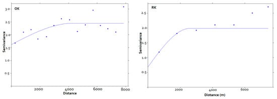
Figure 3.
Semivariogram of SOCS by ordinary kriging (OK) and regression kriging (RK).
3.3.3. Random Forest
The 10-fold cross-validation strategy was implemented in the train function to select the best hyperparameters. The important predictors were sorted in decreasing order of their importance in the variable importance plot (VIP). The MSE in VIP is an informative measure for the selection of variables or the most important prediction factors. VIP revealed different environmental dominances influencing SOCS. It indicated that the distribution of soil organic carbon stocks (SOCS) was largely influenced by the elevation (DEM), coloration index (CI), brightness index (BI), perpendicular vegetation index (PVI), saturation index (SI), soil-adjusted vegetation index (SAVI), and slope (Figure 4). Among the topographic parameters, the elevation and vegetation parameters—CI, BI, and PVI—show relatively large importance, while the remaining covariates are of little contribution for the surface SOCS. Further, these are the important predictors that are responsible for the increase in node purity if taken at the splits.
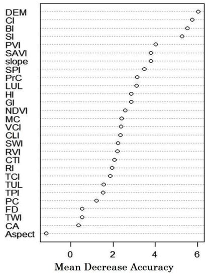
Figure 4.
Variable importance plot—mean decreasing accuracy for SOCS.
The spatial distribution maps by OK, RK, and RF for SOCS are shown in Figure 5. The model prediction of SOCS varied from 0.41 to 56.9 Mg ha−1. The SOCS is little more detailed in RF than OK and RK. RF shows abrupt gradual transition in prediction than the other two, demonstrating the clear influence of auxiliary variables on the spatial variability of SOCS. The transitions are more prominent at the borders of different land uses. The smooth transition along the watershed boundary in all the prediction models is indicative of insufficient sampling intensity.
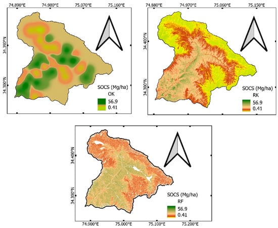
Figure 5.
SOCS (Mg ha−1) maps generated by ordinary kriging (OK), regression kriging (RK), and random forest (RF).
3.4. Model Comparison
The SOCS maps generated using OK, RK, and RF are shown in Figure 5. The predicted models used, viz., ordinary kriging (OK), regression kriging (RK), and random forest (RF), were assessed using RMSE (difference between observed and predicted) and R2 (coefficient of determination) for model comparison. The spatial distribution of SOCS across the complex topography of Wangath was better predicted by RF (RMSE 8.21 and R2 0.9) as compared to OK (RMSE 15.60 and R2 0.53) and RK (RMSE 17.73 and R2 0.29). The prediction accuracy was in the order of RF > OK > RK. The coefficient of determination (R2) of SOCS using RF improved to 0.90, and RMSE was reduced to 8.21 (Table 6).
Table 6.
Performance evaluation of ordinary kriging, regression kriging, and random forest model.
The findings reported by [61,68,69] matched our study. However, OK proved to be better than RK in terms of RMSE and R2; this could be attributed to the fair capturing of the spatial structure by point observations or a weak relationship between auxiliary variables and soil parameters. Similar results were reported by [23,70], that OK proves better in predicting soil properties without using auxiliary variables under higher sampling density and poor spatial correlation between auxiliary variables and the target variable. Gia et al. [17] suggested that a strong and proper selection of the auxiliary can efficiently improve the accuracy of RK, and RK proves a better predictor than OK when the correlation between the target variable and auxiliary variable is >0.50 [6]. The weak spatial structure in a complex topography such as that of the Himalayas is a common feature; thus, a proper selection of auxiliary variables occupies a prominent place in the spatial prediction of soil properties. The three selected models were also assessed using the Taylor diagram (Figure 6), which proved the higher accuracy of RF over the others for SOCS prediction. Similar results were obtained by [71] using the integrated RF-OK (interpolation of RF-residuals by OK) interpolation for SOC even with hyperspectral data [72]. RK performs well when many auxiliary variables with non-linear relationships are used, even under limited soil data. This is because of averaging the output of each tree in RF, while on the other side, the linear model fails to handle the relationship between the target and independent variables [73]. However, given a sizable dataset, the model performance may be comparable [74].
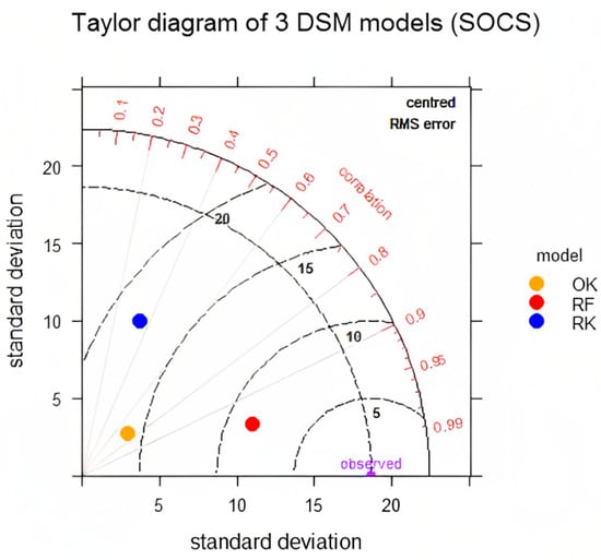
Figure 6.
Taylor diagram of SOCS for the comparative assessment of selected three models: OK, RK, and RF.
4. Conclusions
The scope of DSM in complex topography and land use has not been studied thoroughly. To evaluate and predict how SOCS varies in a complex topography such as that of the Himalayas, the study was conducted in the “Wangath” region of Ganderbal district. Digital Soil Mapping (DSM) methods were used to map the spatial distribution of soil properties, with DEM- and satellite (LANDSAT 8)-derived parameters as environmental covariates. We compared two geostatistical models—ordinary kriging (OK) and regression kriging (RK)—and one machine-learning algorithm—random forest (RF)—for predictive analytics and digital mapping of selected SOCS under highly complex terrain. The geostatistical techniques estimated spatial dependence and variability through semivariogram analysis, indicating a presence of moderate spatial dependence of SOCS in the study area. OK performed better than RK due to the poor spatial correlation between the auxiliary variables and SOCS. However, RF outperformed OK and RK in terms of assessment criteria RMSE and R2. Therefore, RF can be used for the spatial variability assessment of SOCS in such a complex topography and thus could be employed by planners as a decision support tool for farm management and precision agriculture. In future, model-based soil sampling and a precise area of agreement on the study area coverage should be studied to evaluate the effect on the accuracy assessment of the predictive models.
Author Contributions
Conceptualization: S.A.B.; writing, I.F.; review, S.A.B., O.B. and T.I.S.; supervision, A.A.M., A.M.I. and S.S.M.; analysis, S.A.B., A.B., O.A.W. and N.N. All authors have read and agreed to the published version of the manuscript.
Funding
This research received funding from SKUAST Kashmir and project is supported by the Natural Sciences and Engineering Research Council of Canada (NSERC) (RGPIN-2014-4100). The open access fee is supported by the Natural Sciences and Engineering Research Council of Canada (NSERC) (RGPIN-2014-4100).
Institutional Review Board Statement
Not applicable.
Informed Consent Statement
Not applicable.
Data Availability Statement
Data will be made available to the reader upon reasonable request from the corresponding author.
Conflicts of Interest
The authors declare no conflict of interest.
References
- Hussain, S.; Sharma, V.; Arya, V.M.; Sharma, K.R.; Rao, C.S. Total organic and inorganic carbon in soils under different land use/land cover systems in the foothill Himalayas. Catena 2019, 182, 104104. [Google Scholar] [CrossRef]
- Li, L.; Lu, J.; Wang, S.; Ma, Y.; Wei, Q.; Li, X.; Ren, T. Methods for estimating leaf nitrogen concentration of winter oilseed rape (Brassica napus L.) using in situ leaf spectroscopy. Ind. Crop. Prod. 2016, 91, 194–204. [Google Scholar] [CrossRef]
- Antonangelo, J.A.; Sun, X.; Zhang, H. The roles of co-composted biochar (COMBI) in improving soil quality, crop productivity, and toxic metal amelioration. J. Environ. Manag. 2021, 277, 111443. [Google Scholar] [CrossRef] [PubMed]
- Chang, Y.; Rossi, L.; Zotarelli, L.; Gao, B.; Shahid, M.A.; Sarkhosh, A. Biochar improves soil physical characteristics and strengthens root architecture in Muscadine grape (Vitis rotundifolia L.). Chem. Biol. Technol. Agric. 2021, 8, 7. [Google Scholar] [CrossRef]
- Mandal, U.K. Spectral Color Indices Based Geospatial Modeling of Soil Organic Matter in Chitwan District, Nepal. Int. Arch. Photogramm. Remote Sens. Spat. Inf. Sci. 2016, 41, 43–48. [Google Scholar] [CrossRef]
- Bangroo, S.A.; Najar, G.R.; Rasool, A. Effect of altitude and aspect on soil organic carbon and nitrogen stocks in the Himalayan Mawer Forest Range. Catena 2017, 158, 63–68. [Google Scholar] [CrossRef]
- Petermann, E.; Meyer, H.; Nussbaum, M.; Bossew, P. Mapping the geogenic radon potential for Germany by machine learning. Sci. Total Environ. 2021, 754, 142291. [Google Scholar] [CrossRef]
- Swiderski, B.; Osowski, S.; Kruk, M.; Barhoumi, W. Aggregation of classifiers ensemble using local discriminatory power and quantiles. Expert Syst. Appl. 2016, 46, 316–323. [Google Scholar] [CrossRef]
- Bashir, O.; Ali, T.; Baba, Z.A.; Rather, G.H.; Bangroo, S.A.; Mukhtar, S.D.; Naik, N.; Mohiuddin, R.; Bharati, V.; Bhat, R.A. Soil Organic Matter and Its Impact on Soil Properties and Nutrient Status. In Microbiota and Biofertilizers; Springer: Berlin/Heidelberg, Germany, 2021; Volume 2, pp. 129–159. [Google Scholar]
- Batjes, N.H. Total carbon and nitrogen in the soils of the world. Eur. J. Soil Sci. 1996, 47, 151–163. [Google Scholar] [CrossRef]
- Webster, R.; Oliver, M.A. Geostatistics for Environmental Scientists; John Wiley & Sons: Hoboken, NJ, USA, 2007. [Google Scholar]
- Zhang, C.; Tang, Y.; Xu, X.; Kiely, G. Towards spatial geochemical modelling: Use of geographically weighted regression for mapping soil organic carbon contents in Ireland. Appl. Geochem. 2011, 26, 1239–1248. [Google Scholar] [CrossRef]
- Ma, S.; Qiao, Y.P.; Wang, L.J.; Zhang, J.C. Terrain gradient variations in ecosystem services of different vegetation types in mountainous regions: Vegetation resource conservation and sustainable development. For. Ecol. Manag. 2021, 482, 118856. [Google Scholar] [CrossRef]
- Lagacherie, P.; McBratney, A.B. Spatial soil information systems and spatial soil inference systems: Perspectives for digital soil mapping. Dev. Soil Sci. 2006, 31, 3–22. [Google Scholar]
- Reza, S.K.; Nayak, D.C.; Chattopadhyay, T.; Mukhopadhyay, S.; Singh, S.K. Srinivasan, R. Spatial distribution of soil physical properties of alluvial soils: A geostatistical approach. Arch. Agron. Soil Sci. 2016, 62, 972–981. [Google Scholar] [CrossRef]
- Zhang, H.; Wu, P.; Yin, A.; Yang, X.; Zhang, M.; Gao, C. Prediction of soil organic carbon in an intensively managed reclamation zone of eastern China: A comparison of multiple linear regressions and the random forest model. Sci. Total Environ. 2017, 592, 704–713. [Google Scholar] [CrossRef]
- Pham, T.G.; Kappas, M.; Van Huynh, C.; Nguyen, L.H.K. Application of ordinary kriging and regression kriging method for soil properties mapping in hilly region of Central Vietnam. ISPRS Int. J. Geo-Inf. 2019, 8, 147. [Google Scholar] [CrossRef]
- Duffera, M.; White, J.G.; Weisz, R. Spatial variability of Southeastern US Coastal Plain soil physical properties: Implications for site-specific management. Geoderma 2007, 137, 327–339. [Google Scholar] [CrossRef]
- Fathololoumi, S.; Vaezi, A.R.; Alavipanah, S.K.; Ghorbani, A.; Saurette, D.; Biswas, A. Effect of multi-temporal satellite images on soil moisture prediction using a digital soil mapping approach. Geoderma 2021, 385, 114901. [Google Scholar] [CrossRef]
- Keerthan, K.; Shubha, T.G.; Sushma, S.A. Random forest algorithm for soil fertility prediction and grading using machine learning. Int. J. Innov. Technol. Explor. Eng. 2019, 9, 1301–1304. [Google Scholar]
- Heuvelink, G.B.M.; Webster, R. Modelling soil variation: Past, present, and future. Geoderma 2001, 100, 269–301. [Google Scholar] [CrossRef]
- Wiesmeier, M.; Barthold, F.; Blank, B.; Kögel-Knabner, I. Digital mapping of soil organic matter stocks using Random Forest modeling in a semi-arid steppe ecosystem. Plant Soil 2011, 340, 7–24. [Google Scholar] [CrossRef]
- Pouladi, N.; Møller, A.B.; Tabatabai, S.; Greve, M.H. Mapping soil organic matter contents at field level with Cubist, Random Forest and kriging. Geoderma 2019, 342, 85–92. [Google Scholar] [CrossRef]
- Wiesmeier, M.; Urbanski, L.; Hobley, E.; Lang, B.; von Lützow, M.; Marin-Spiotta, E.; van Wesemael, B.; Rabot, E.; Ließ, M.; Garcia-Franco, N.; et al. Soil organic carbon storage as a key function of soils-A review of drivers and indicators at various scales. Geoderma 2019, 333, 149–162. [Google Scholar] [CrossRef]
- Yang, Z.; Di, L.; Yu, G.; Chen, Z. Vegetation condition indices for crop vegetation condition monitoring. In Proceedings of the 2011 IEEE International Geoscience and Remote Sensing Symposium, Vancouver, BC, Canada, 24–29 July 2011; pp. 3534–3537. [Google Scholar]
- Huang, H.; Chen, Y.; Clinton, N.; Wang, J.; Wang, X.; Liu, C.; Gong, P.; Yang, J.; Bai, Y.; Zheng, Y.; et al. Mapping major land cover dynamics in Beijing using all Landsat images in Google Earth Engine. Remote Sens. Environ. 2017, 202, 166–176. [Google Scholar] [CrossRef]
- Moore, I.D.; Gessler, P.E.; Nielsen, G.A.E.; Peterson, G.A. Soil attribute prediction using terrain analysis. Soil Sci. Soc. Am. J. 1993, 57, 443–452. [Google Scholar] [CrossRef]
- Baltensweiler, A.; Walthert, L.; Hanewinkel, M.; Zimmermann, S.; Nussbaum, M. Machine learning based soil maps for a wide range of soil properties for the forested area of Switzerland. Geoderma Reg. 2021, 27, e00437. [Google Scholar] [CrossRef]
- Wang, S.; Huang, M.; Shao, X.; Mickler, R.A.; Li, K.; Ji, J. Vertical distribution of soil organic carbon in China. Environ Manag. 2004, 33, S200–S209. [Google Scholar] [CrossRef]
- Liu, Z.; Liu, Q. Magnetic properties of two soil profiles from Yan’an, Shaanxi Province and their implications for paleorainfall reconstruction. Sci. China Earth Sci. 2014, 57, 719–728. [Google Scholar] [CrossRef]
- Brungard, C.W.; Boettinger, J.L.; Duniway, M.C.; Wills, S.A.; Edwards, T.C., Jr. Machine learning for predicting soil classes in three semi-arid landscapes. Geoderma 2015, 239, 68–83. [Google Scholar] [CrossRef]
- Tarboton, D.G.; Dash, P.; Sazib, N. TauDEM 5.3: Guide to Using the TauDEM Command Line Functions. 2015. Available online: https://hydrology.usu.edu/taudem/taudem5/TauDEM53CommandLineGuide.pdf (accessed on 13 July 2021).
- Tahir, M.; Imam, E.; Hussain, T. Evaluation of land use/land cover changes in Mekelle City, Ethiopia using Remote Sensing and GIS. Comput Ecol Softw. 2013, 3, 9. [Google Scholar]
- Nelson, D.W.; Sommers, L. Total carbon, organic carbon, and organic matter. Method. Soil Anal. Part 2 Chem. Microbiol. Prop. 1983, 9, 539–579. [Google Scholar]
- Blake, G.R.; Hartge, K.H. Bulk Density. In Methods of Soil Analysis, Part I Physical and Mineralogical Methods, 2nd ed.; Klute, A., Ed.; ASA-SSSA: Madison, WI, USA, 1986; pp. 363–375. [Google Scholar] [CrossRef]
- Penman, J.; Gytarsky, M.; Hiraishi, T.; Krug, T.; Kruger, D.; Pipatti, R.; Buendia, L.; Miwa, K.; Ngara, T.; Tanabe, K.; et al. Good Practice Guidance for Land Use, Land Use Change and Forestry; Institute for Global Environmental Strategies: Hayama, Japan, 2003. [Google Scholar]
- Khan, N.M.; Rastoskuev, V.V.; Sato, Y.; Shiozawa, S. Assessment of hydro saline land degradation by using a simple approach of remote sensing indicators. Agric. Water Manag. 2005, 77, 96–109. [Google Scholar] [CrossRef]
- Gitelson, A.A.; Kaufman, Y.J.; Merzlyak, M.N. Use of a green channel in remote sensing of global vegetation from EOS-MODIS. Remote Sens. Environ. 1996, 58, 289–298. [Google Scholar] [CrossRef]
- Gao, B.C. NDWI—A normalized difference water index for remote sensing of vegetation liquid water from space. Remote Sens. Environ. 1996, 58, 257–266. [Google Scholar] [CrossRef]
- Liu, W.T. Kogan, F.N. Monitoring regional drought using the Vegetation Condition Index. Int. J. Remote Sens. 1996, 17, 2761–2782. [Google Scholar] [CrossRef]
- Rouse, J.W.; Haas, R.; Schell, J.; Deering, D. Monitoring vegetation systems in the great plains with erts. NASA Spec. Publ. 1974, 351, 309–317. [Google Scholar]
- Mathieu, R.; Pouget, M.; Cervelle, B.; Escadafal, R. Relationships between Satellite-Based Radiometric Indices Simulated Using Laboratory Reflectance Data and Typic Soil Color of an Arid Environment. Remote. Sens. Environ. 1998, 66, 17–28. [Google Scholar] [CrossRef]
- Pearson, R.L.; Miller, L.D. Remote Mapping of Standing Crop Biomass for Estimation of the Productivity of the Short-Grass Prairie. In Proceedings of the Eighth International Symposium on Remote Sensing of Environment, Pawnee National Grasslands, Colorado, Ann Arbor, MI, USA, 2–6 October 1972; pp. 357–1381. [Google Scholar]
- Amro, F.A. Using Remote Sensing data to identify iron deposits in central western Libya. In Proceedings of the International Conference on Emerging Trends in Computer and Image Processing (ICETCIP 2011), Bangkok, Thailand, 23–24 December 2011. [Google Scholar]
- Richardson, A.J.; Wiegand, C.L. Distinguishing vegetation from soil background information. Photogramm. Eng. Remote Sens. 1977, 43, 1541–1552. [Google Scholar]
- Huete, A.R. A soil-adjusted vegetation index (SAVI). Remote Sens. Environ. 1988, 25, 295–309. [Google Scholar] [CrossRef]
- Prodanovic, D.; Stanic, M.; Milivojevic, V.; SimiC, Z.; ArsiC, M. DEM-Based GIS Algorithms for Automatic Creation of Hydrological Models Data. J. Serb. Soc. Comput. Mech. 2009, 3, 64–85. [Google Scholar]
- Wilson, J.P.; Gallant, J.C. (Eds.) Terrain analysis: Principles and applications; John Wiley & Sons: Hoboken, NJ, USA, 2000. [Google Scholar]
- Jenness, J. Topographic Position Index (tpi_jen.avx) extension for ArcView 3.x, v. 1.2. Jenness Enterprises. 2006. Available online: http://www.jennessent.com/arcview/tpi.htm (accessed on 13 July 2021).
- Boehner, J.; Koethe, R.; Conrad, O.; Gross, J.; Ringeler, A.; Selige, T. Soil Regionalisation by Means of Terrain Analysis and Process Parameterisation. In Soil Classification 2001; European Soil Bureau, Research Report No. 7, EUR 20398 EN; Micheli, E., Nachtergaele, F., Montanarella, L., Eds.; Office for Official Publications of the European Communities: Luxembourg, 2002; pp. 213–222. [Google Scholar]
- Moore, I.D.; Grayson, R.B.; Ladson, A.R. Digital Terrain Modelling: A Review of Hydrological, Geomorphological, and Biological Applications. Hydrol. Process. 1991, 5, 3–30. [Google Scholar] [CrossRef]
- Erskine, R.H.; Green, T.R.; Ramirez, J.A.; MacDonald, L.H. Comparison of grid-based algorithms for computing upslope contributing area. Water Resour. Res. 2006, 42, W09416. [Google Scholar] [CrossRef]
- Moore, I.D.; Wilson, J.P. Length-slope factors for the revised universal soil loss equation: Simplified method of estimation. J. Soil Water Conserv. 1992, 47, 423–428. [Google Scholar]
- Moore, I.D.; Burch, G.J. Modelling Erosion and Deposition: Topographic Effects. Trans. ASAE 1986, 29, 1624–1630. [Google Scholar] [CrossRef]
- Moore, I.D.; Turner, A.K.; Wilson, J.P.; Jenson, S.K.; Band, L.E. GIS and land-surface-subsurface process modelling. In Environmental Modelling with GIS; Goodchild, M.F., Parks, B.O., Steyaert, L.T., Eds.; CRC Press: Boca Raton, FL, USA, 1993; pp. 213–230. [Google Scholar]
- Bai, T.; Tahmasebi, P. Accelerating geostatistical modeling using geostatistics-informed machine Learning. Comput Geosci. 2021, 146, 104663. [Google Scholar] [CrossRef]
- Das, S. Extreme rainfall estimation at ungauged locations: Information that needs to be included in low-lying monsoon climate regions like Bangladesh. J. Hydrol. 2021, 601, 126616. [Google Scholar] [CrossRef]
- Brunello, A.; Urgolo, A.; Pittino, F.; Montvay, A.; Montanari, A. Virtual Sensing and Sensors Selection for Efficient Temperature Monitoring in Indoor Environments. Sensors 2021, 21, 2728. [Google Scholar] [CrossRef]
- Cambardella, C.A.; Moorman, T.B.; Parkin, T.B.; Karlen, D.L.; Novak, J.M.; Turco, R.F.; Konopka, A.E. Field-scale variability of soil properties in central Iowa soils. Soil Sci. Soc. Am. J. 1994, 58, 1501–1511. [Google Scholar] [CrossRef]
- Heung, B.; Bulmer, C.E.; Schmidt, M.G. Predictive soil parent material mapping at a regional-scale: A random forest approach. Geoderma 2014, 214, 141–154. [Google Scholar] [CrossRef]
- Rokni, K.; Ahmad, A.; Selamat, A.; Hazini, S. Water feature extraction and change detection using multitemporal Landsat imagery. Remote Sens. 2014, 6, 4173–4189. [Google Scholar] [CrossRef]
- Taylor, K.E. Summarizing multiple aspects of model performance in a single diagram. J. Geophys. Res. Atmos. 2001, 106, 7183–7192. [Google Scholar] [CrossRef]
- R Core Team R: A Language and Environment for Statistical Computing. R Foundation for Statistical Computing, Vienna, Austria. 2020. Available online: https://www.R-project.org/ (accessed on 15 March 2021).
- Denton, O.A.; Aduramigba-Modupe, V.O.; Ojo, A.O.; Adeoyolanu, O.D.; Are, K.S.; Adelana, A.O.; Oke, A.O. Assessment of spatial variability and mapping of soil properties for sustainable agricultural production using geographic information system techniques (GIS). Cogent Food Agric. 2017, 3, 1279366. [Google Scholar] [CrossRef]
- Wan, Y.; Lin, E.; Xiong, W.; Guo, L. Modeling the impact of climate change on soil organic carbon stock in upland soils in the 21st century in China. Agric. Ecosyst. Environ. 2011, 141, 23–31. [Google Scholar] [CrossRef]
- Liu, S.; An, N.; Yang, J.; Dong, S.; Wang, C.; Yin, Y. Prediction of soil organic matter variability associated with different land use types in mountainous landscape in southwestern Yunnan province, China. Catena 2015, 133, 137–144. [Google Scholar] [CrossRef]
- McNicol, G.; Bulmer, C.; D’Amore, D.; Sanborn, P.; Saunders, S.; Giesbrecht, I.J.; Arriola, S.G.; Bidlack, A.; Butman, D.; Buma, B. Large, climate-sensitive soil carbon stocks mapped with pedology-informed machine learning in the North Pacific coastal temperate rainforest. Environ. Res. Lett. 2019, 14, 014004. [Google Scholar] [CrossRef]
- Kumar, S.; Lal, R. Mapping the organic carbon stocks of surface soils using local spatial interpolator. J. Environ. Monit. 2011, 13, 3128–3135. [Google Scholar] [CrossRef] [PubMed]
- Zhang, P.; Guo, Z.; Ullah, S.; Melagraki, G.; Afantitis, A.; Lynch, I. Nanotechnology and artificial intelligence to enable sustainable and precision agriculture. Nat. Plants 2021, 7, 864–876. [Google Scholar] [CrossRef] [PubMed]
- Qu, Y.; Zhu, Z.; Montzka, C.; Chai, L.; Liu, S.; Ge, Y.; Liu, J.; Lu, Z.; He, X.; Zheng, J.; et al. Inter-comparison of several soil moisture downscaling methods over the Qinghai-Tibet Plateau, China. J. Hydrol. 2020, 592, 125616. [Google Scholar] [CrossRef]
- Gasmi, A.; Gomez, C.; Chehbouni, A.; Dhiba, D.; El Gharous, M. Using PRISMA Hyperspectral Satellite Imagery and GIS Approaches for Soil Fertility Mapping (FertiMap) in Northern Morocco. Remote Sens. 2022, 14, 4080. [Google Scholar] [CrossRef]
- Gomez, C.; Rossel, R.A.V.; McBratney, A.B. Soil organic carbon prediction by hyperspectral remote sensing and field vis-NIR spectroscopy: An Australian case study. Geoderma 2008, 146, 403–411. [Google Scholar] [CrossRef]
- Sekulic, A.; Kilibarda, M.; Heuvelink, G.B.M.; Nikolic, M.; Bajat, B. Random Forest Spatial Interpolation. Remote. Sens. 2020, 12, 1687. [Google Scholar] [CrossRef]
- Wadoux, A.M.J.C.; Brus, D.J.; Heuvelink, G.B.M. Sampling design optimization for soil mapping with random forest. Geoderma 2019, 355, 113913. [Google Scholar] [CrossRef]


Publisher’s Note: MDPI stays neutral with regard to jurisdictional claims in published maps and institutional affiliations. |
© 2022 by the authors. Licensee MDPI, Basel, Switzerland. This article is an open access article distributed under the terms and conditions of the Creative Commons Attribution (CC BY) license (https://creativecommons.org/licenses/by/4.0/).