Spatiotemporal Dynamics of Soil Impermeability and Its Impact on the Hydrology of An Urban Basin

Abstract

The presence of impervious surfaces in catchments interferes with the natural process of infiltration, which has a marked influence on the hydrological cycle, affecting the base flow in rivers and increasing the surface runoff and the magnitude of flood flows. Like many Latin American cities, Loja (located in southern Ecuador) has experienced significant rates of urban growth in recent years, increasing the impervious surfaces in the catchment where it belongs. The aim of this study is to analyze the spatiotemporal dynamics of imperviousness in the study area for the period 1989–2020, using the Normalized Difference Impervious Surface Index (NDISI) and the supervised classification of Landsat images. The effect on flood flows was studied for each timestep using HEC-HMS hydrological model. Additionally, a future scenario of impervious surfaces was generated considering the observed spatiotemporal variability, possible explanatory variables, and logistic regression models. Between 1989 and 2020, there was an increase of 144.12% in impervious surfaces, which corresponds to the population growth of 282.56% that occurred in the same period. The period between 2001 and 2013 was the one that presented the most significant increase (1.06 km²/year). A direct relationship between the increase in impervious surfaces and the increase in flood flows was observed, reaching a significant variation towards the horizon year that could affect the population, for which measures to manage the surface runoff is necessary.

1. Introduction

Features such as climate, topography, vegetation, and coverage of a natural watershed produce a natural water cycle and a given hydrological response. Different factors such as the impervious surfaces can affect this unique natural hydrological process and cause adverse effects to the catchment [1].

The impervious surface is usually defined as the collection of anthropogenic landforms that water cannot directly infiltrate into, including rooftops, roads, and parking lots [2,3]. The urbanization process has significant impacts on the hydrology of a basin; as urban areas expand, permeable and moisture-holding lands transform into impervious surfaces such as concrete and asphalt, causing a decrease in infiltration and base flow, as well as an increase in flood flows and runoff volumes. The storm drainage systems simplify the natural drainage systems, altering the response of the basin to precipitation events since shorter concentration and recession times occur [1,4,5]. On the other hand, the dynamics of impervious surfaces impact urban regional climate by altering the thermal environment and water quality [3,6].

Several studies have analyzed the effect of urbanization [7,8,9], land-use changes [10,11,12,13,14], or impervious cover change [15,16] on Hydrology.

Remote sensing has been extensively utilized for the detection of impervious surfaces [17,18]. The approaches have been diverse: index-based methods, classification-based methods, and mixture analysis. The index-based methods include indices such as normalized difference buildup index (NDBI) [19], normalized difference impervious surface index (NDISI) [20], modified NDISI (MNDISI) [21], biophysical composition index (BCI) [22], and perpendicular impervious surface index (PISI) [23]. The classification and regression approaches include maximum likelihood classifier [24], support vector machine [25], artificial neural networks [26], random forest [27], and object-oriented methods [28]. For the mixture analysis, spectral mixture analysis (SMA) [29] and temporal mixture analysis (TMA) [30] are applied.

Urbanization is a worldwide trend. Currently, more than 50% of the world’s population lives in urban centers, and more than 500 cities in the world have a population above 1 million inhabitants [5]. The reasons for urban growth are diverse; in Latin American cities, we could highlight the natural demographic growth, migration from the countryside to the city in search of better living conditions, changes in the location patterns of economic activities, and housing, among others.

Several cities in Ecuador have experienced rapid growth, which is evidenced in a notable increase in the urbanized area in recent years. One of those cities is Loja, capital of the province of the same name, located south of Ecuador and bordering Peru. This study analyzes the influence of urban growth on the hydrology of the basin where the city is located and on the extreme flow events that occur in it. For this, using aerial photographs and satellite images, a Normalized Difference Impervious Surface Index (NDISI) was calculated, and a multitemporal analysis of the urban surface variation was carried out. Then, flood flows for various coverage scenarios were generated using precipitation data and applying a hydrological model to finally evaluate the effect of these flows over the areas surrounding the riverbanks in various points of interest. The study of the spatiotemporal variation of the impervious surfaces using a spectral index and supervised classification of images, combined with statistical techniques and artificial intelligence to define future scenarios of impervious surfaces, and the evaluation of their possible impacts through hydrological modeling, are the newest aspects of the present work.

2. Materials and Methods

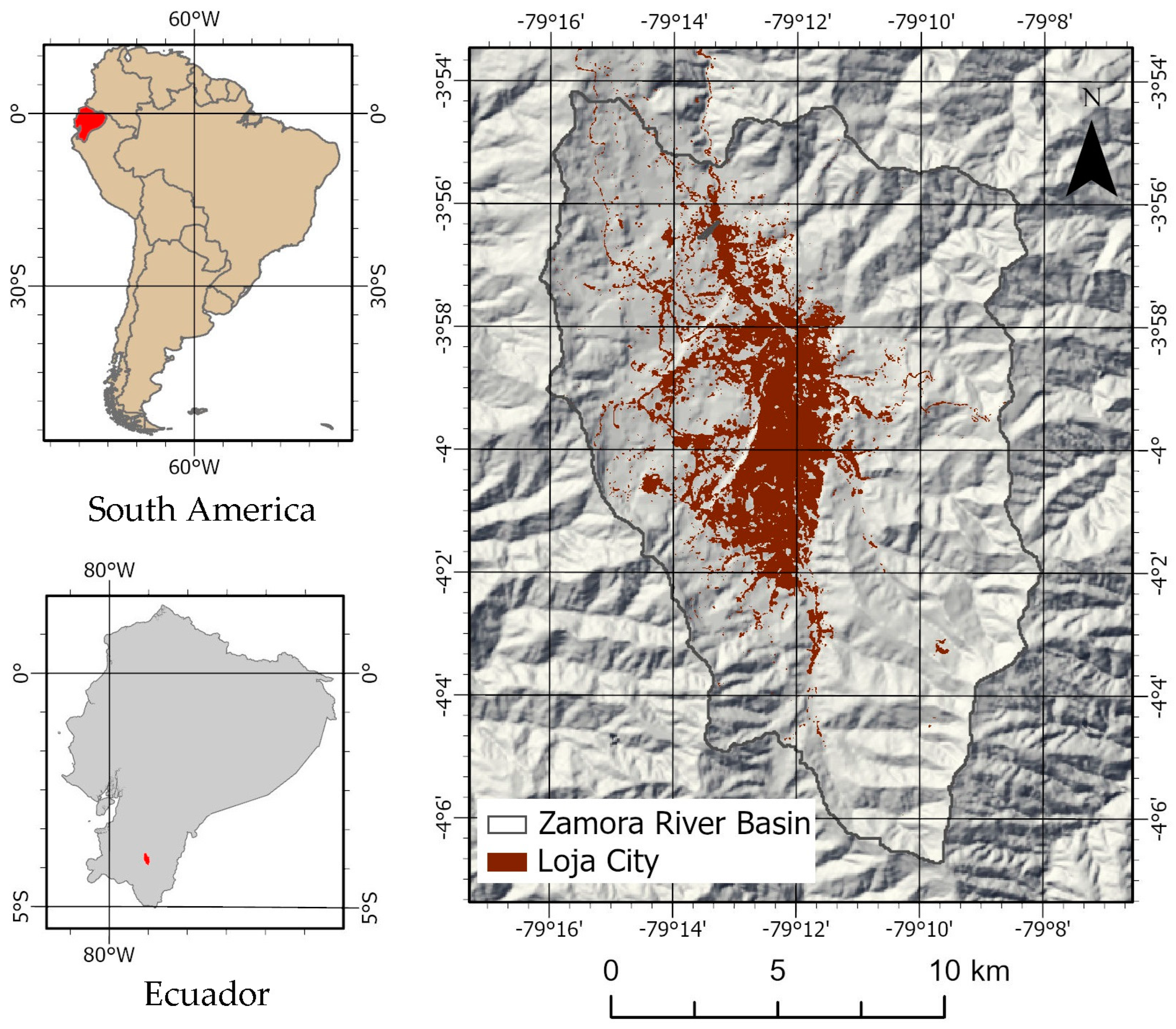
2.1. Study Area

The Zamora River (A = 227 km²) is a tributary of the Santiago River and part of the hydrological system of the Amazon River. The Zamora River basin is located in the southern Andes of Ecuador, has an average height of 2400 m above sea level, an average slope of 30%, and an average slope of the main channel of 8.3% [31]. The basin is covered by vegetation in good condition, mainly composed of grasslands, scrublands, and forests [32]. Its climate is subhumid equatorial temperate, with a mean annual precipitation depth of 909.1 mm. The Zamora River presents dry periods between May and November and can present important flows during the rainy season (from December to April) [33]. The Zamora River, up to its pour point (79°13′28″ W, 3°55′17″ S) has six main tributaries that make up a network of 102.70 km in length, with the main channel of 22.89 km, which has stream order three, according to the Horton—Strahler Laws. The city of Loja occupies the middle and lower portion of the basin. The city has about 200,000 inhabitants and an area of 43 km², being the only existing urban area in the Zamora River basin. The growth of the city in the last 30 years, as well as the construction and improvement of the road network, has created impervious zones.

The location of the study area is presented in Figure 1.

2.2. Data Collection

Three image sets, acquired from Landsat 5 Thematic Mapper (TM), Landsat 7 Enhanced Thematic Thematic Mapper Plus (ETM+), and Landsat 8 Operational Land Imager (OLI)-Thermal Infrared Sensor (TIRS) were collected in the study area [34]. Their acquisition dates, spectral bands, and spatial resolutions are listed in

Table 1. Satellite images from the three Landsat sensors (TM, ETM+, OLI-TIRS) used in this study.

Satellite	Sensor	Acquisition Date	Resolution (m)	Wavelength (μm)
Landsat-5	TM	10 November 1989	30	Band1 (Blue): 0.441–0.514
				Band2 (Green): 0.519–0.601
				Band3 (Red): 0.631–0.692
				Band4 (NIR): 0.772–0.898
				Band5 (SWIR-1): 1.547–1.749
			120	Band6 (TIR): 10.31–12.36
			30	Band7 (SWIR-2): 2.064–2.345
Landsat-7	ETM+	3 November 2001	30	Band1 (Blue): 0.441–0.514
				Band2 (Green): 0.519–0.601
				Band3 (Red): 0.631–0.692
				Band4 (NIR): 0.772–0.898
				Band5 (SWIR-1): 1.547–1.749
			60	Band6 (TIR): 10.31–12.36
			30	Band7 (SWIR-2): 2.064–2.345
			15	Band8 (Pan): 0.515–0.896
Landsat-8	OLI-TIRS	28 November 2013 11 August 2020	30	Band1 (Coastal/Aerosol): 0.435–0.451
				Band2 (Blue): 0.452–0.512
				Band3 (Green): 0.533–0.590
				Band4 (Red): 0.636–0.673
				Band5 (NIR): 0.851–0.879
				Band6 (SWIR-1): 1.566–1.651
				Band7 (SWIR-2): 2.107–2.294
			15	Band8 (Pan): 0.503–0.676
			30	Band9 (Cirrus): 1.363–1.384
			100	Band10 (TIR-1): 10.60–11.19
				Band11 (TIR-2): 11.50–12.51

. Atmospheric correction was performed to each image using the Atmospheric/Topographic Correction for Mountainous Terrain (ATCOR) software developed by the German Aerospace Center, Wessling, Germany [35]. The Landsat images archived in the U.S. Geological Survey (USGS) data clearinghouse have been georectified [36]. All images in Table 1 are geometrically matched to each other.

Further, historical information on the type and land use of the study area was collected [37], which was used in the hydrological modeling component of this study.

2.3. Analysis of Impervious Surfaces

The Normalized Difference Impervious Surface Index (NDISI) [20,38] is used to enhance impervious surfaces and suppress land covers such as soil, sand, and water bodies.

$$NDISI=\frac{T_b-\left(MNDWI+NIR+SWIR1\right)/3}{T_b+\left(MNDWI+NIR+SWIR1\right)/3}$$

(1)

T_b refers to the brightness temperature of the TIRS1 thermal band. MNDWI represents the Modified Normalized Difference Water Index (Equation (2)), NIR refers to the pixel values extracted from the near-infrared band. SWIR1 refers to the pixel values extracted from the first shortwave infrared band.

$$MNDWI=\frac{G-SWIR1}{G+SWIR1}$$

(2)

G represents the pixel values extracted from the green band.

Applying Equation (1), NDISI images were generated for each of the collected images (Table 1). A manually adjusted threshold was used to extract impervious surface features from the NDISI images generated. The pixels with values greater than the threshold are impervious surfaces and were assigned a value of 1, while the pixels with values equal to or less than the threshold are nonimpervious surfaces and were assigned a value of 0. Thus, the resultant image is a binary image, only showing the extracted impervious surfaces.

Additionally, the supervised classification of the collected images was carried out using the maximum likelihood method [39] in order to obtain the urban area (impervious surface) and its temporal variation and maps of the impervious and nonimpervious surface for the study area.

The performance of the NDISI and the supervised classification for the detection of impervious surfaces was evaluated by visual comparison with the images included in Table 1. Using the results of the technique that offered the most reliable results, the spatiotemporal analysis was performed, as well as the generation of scenarios towards the year 2030 and hydrological modeling in order to study the impact of the variation of impervious surfaces on the hydrology of the basin under study.

2.4. Spatiotemporal Analysis of Impervious Surfaces and Scenario Generation

Once the maps of the impervious and nonimpervious surface were obtained, the changes that occurred between 1989 and 2001 were analyzed, relating them to the possible explanatory variables to obtain a predictive model that could be validated by comparison with the coverage obtained for 2013.

The changes that occurred were studied by applying the methodology proposed by [40], which allows determining the persistence, gain, loss, and exchanges between the thematic categories considered in each land occupation map through the analysis of a cross-tabulation, identifying the transitions that occurred between 1989 and 2001. The relationships between the observed transitions and their possible explanatory variables are called transition submodels. The number of transition submodels will be equal to the number of transitions that occur in the study area; it is possible to group several transitions into a single model when it is considered that these are the product of the same causes. Each transition model includes a certain number of explanatory variables, which can be selected based on their explanatory potential, calculated by Cramer’s V coefficient, or by testing various combinations of explanatory variables until the optimal fit between transitions and explanatory variables is obtained. Cramer’s V values greater than 0.4 are acceptable [41]. Three explanatory variables were considered: Elevation (using a digital elevation model—DEM), which influences the presence of different types of vegetation; the slope, which limits urban growth; and the distance to streets and roads, which motivates and facilitates urban growth.

The transition submodels were calculated by logistic regression and by means of a multilayer perceptron neural network (MLP), obtaining the probability of occurrence of each transition according to the selected explanatory variables. Logistic regression [42] allows establishing a relationship between a binary dependent variable (transitions) and the explanatory variables considered, modeling their probability of occurrence according to the latter.

Neural networks of multilayer perceptrons are formed by a set of simple elements (neurons or perceptrons) distributed in layers and are connected to the intermediate layer or layers by means of activation functions. These functions are defined from a series of weights or weighting factors that are calculated interactively in the learning process of the network. The objective of this learning is to estimate known results (observed transitions) from some input data (explanatory variables); to later calculate unknown results from the rest of the input data. Learning is carried out from all the units that make up the network, varying the set of weights in successive interactions [39].

The land cover change modeling towards the horizon year (2013) was carried out applying Markov chains; using the land cover map of the end date (2001) along with the transition probability matrix previously calculated, to determine the zones are that will undergo a transition from the end date to the prediction date (2013).

The future land cover map was modeled using a multiobjective land-use allocation procedure (MOLA) [41,43]. Considering all transitions and using the selected explanatory variables, a list of host classes (which would lose some area) and a list of demanding classes (which would gain some area) are created. Loss or gain areas are determined by Markov chains and through the multiobjective allocation procedure, in which the explanatory variables determine the most suitable places for each change in occupation. Land from all host classes is allocated to all demanding classes. The results of each land occupation reallocation are overlaid to produce the final result [41]

Two maps were generated to predict land cover for the year 2013 based on the modeling of the relationships between the observed changes and the explanatory variables. These relationships were modeled with logistic regression and neural networks. For the validation, the map extracted from the 2013 image was considered as a reference, and, through confusion matrices, the correspondence between the reference map and those obtained through neural networks and logistic regression was studied. Forecast errors of land cover were determined for each model proposed, as well as omission and commission errors that may have occurred.

From the confusion matrix, the global reliability of the classification was calculated as the relationship between the number of pixels correctly assigned and the total number of pixels in the image [39]. Complementarily, the fit between the reference map and the maps generated was calculated using the Kappa index [40]. After analyzing the adjustment, we proceeded to generate a land cover map towards the year 2030, considering the land cover maps of 2013 and 2020, the explanatory variables selected for each transition, and applying the model that presents the best capacities.

The spatiotemporal analysis of impervious surfaces and scenario generation described was carried out by applying the land change modeler module of TerrSet 2020 [41].

2.5. Hydrological Modeling

The HEC-HMS model was developed to study the response of the Zamora River basin to extreme precipitation events, considering the different stages of urban growth in the city of Loja. The basin topology was developed based on a digital elevation model generated using a contour map at 1:50,000 scale [44]. This topological model included contributing sub-basins, junction points in which the contributions of the sub-basins are added, sections of the river network in which the hydrologic routing of the hydrographs is carried out, and the outlet point of the basin in which the flow resulting from the rain-runoff simulation is obtained. The topological model is presented in Figure 2.

Synthetic storms were generated for return periods of 10, 25, 50, and 100 years, using intensity equations determined for the city of Loja [45].

$$I_{TR}=92.854I{d}_{TR}{t}^{-0.4083}$$

(3)

$$I_{TR}=480.74I{d}_{TR}{t}^{-0.8489}$$

(4)

where Id_TR is the maximum intensity for a given return period, t is the duration of the storm in minutes, I_TR is the intensity in mmh⁻¹. Equation (1) is valid for durations between 5 and 43 min, Equation (2) is valid for durations between 43 min and 1440 min.

Abstractions were quantified using the curve number (CN) methodology of the U.S. Soil Conservation Service (USSCS) [4,46] for normal conditions, calculating the CN for each hydrological response unit obtained according to the intersection of type and land use for each date considered. The transformation of surface runoff into flow was carried out by applying the USSCS Unit Hydrograph. For the hydrologic flow routing, the Muskingum-Cunge method was applied. The concentration and delay times of each sub-basins were determined using the Kirpich formula [4,46].

3. Results and Analysis

3.1. Analysis of Impervious Surfaces Using NDISI

Figure 3 shows the temporal variation of the NDISI index. A visual comparison with the collected images allowed us to determine that the consolidated areas of the city center are identified in an acceptable way through the NDISI index. The areas surrounding the city center were consolidated as urban areas over time, and in the process, a transition is observed from the heterogeneous mixture of impervious and green areas to consolidated urban areas. The impervious surfaces of the southwestern portion of the city were underestimated in all analyzed images. Land surface emissivity (ε) varies with land cover on the ground surface. In urban environments, surfaces with vegetation have a higher thermal retention capacity and, therefore, have greater cooling effects than areas without vegetation [47], which is reflected in the temporal variation of the NDISI.

In suburban–rural areas, impervious areas have been identified to the west of the city. These areas do not correspond to urban areas but to surfaces with bare soil due to fallow agricultural areas or small areas under construction that have just been cleared. On the other hand, the selected images were taken between August and November (which are part of the dry season) to ensure less cloud cover. Therefore, during that period, the vegetation cover is less vigorous and frequently leaves the soil exposed. In Landsat images, bare soil is often mistaken for impervious surfaces due to their similar spectral characteristics, resulting in noisy salt and pepper appearances in supervised image classification [47]. Furthermore, the thermal response of the soil is quite similar to that of the impermeable surface, which causes spectral confusion between impermeable areas and bare soil when classifying it [20,48].

Despite its acceptable performance, it was considered that the NDISI and its temporal analysis were not completely adequate to study the evolution of the impervious surfaces in the study area.

3.2. Analysis of Impervious Surfaces by Supervised Classification

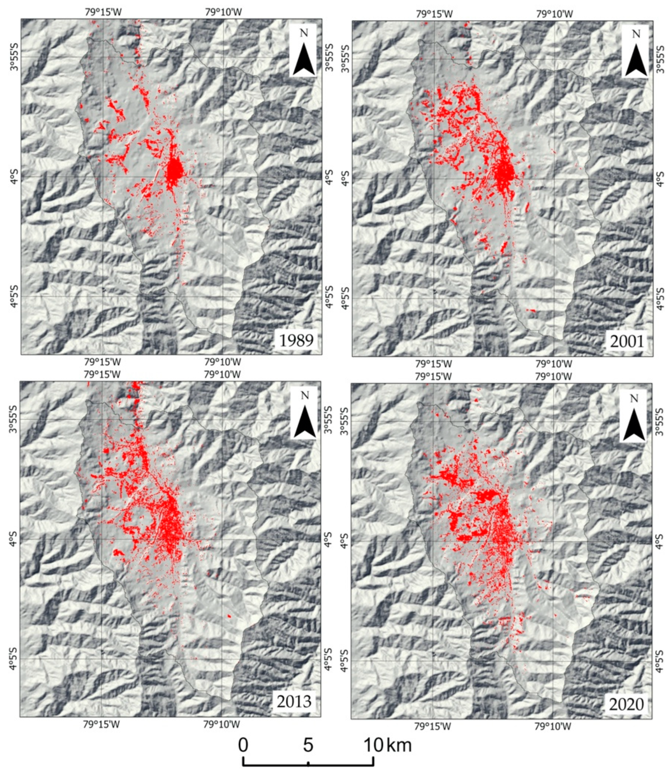
Figure 4 shows the impervious surfaces in the study area determined by supervised classification applying the maximum likelihood criterion. A visual comparison with the collected images shows an adequate representation of the impervious surfaces and their spatiotemporal variation, which is why they are selected for the following phases of the study.

A summary of the area occupied by the city (impervious surfaces) and its respective population at each year considered is included in

Table 2. Variation of urban area and population in the city of Loja. Period 1989–2020.

Year	Impervious Surface			Population
	Area (km2)	Increase (%) *	Annual (km2/year)	Total (PPL)	Increase (%) *	Density (PPL/km2)
1989	17.68	0	0	71,652	0	4052.71
2001	20.18	14.17	0.21	118,532	65.43	5873.74
2013	32.87	85.97	1.06	185,321	158.64	5638.00
2020	43.15	144.12	1.47	274,112	282.56	6352.54

* Reference year: 1989.

.

Table 2 includes a summary of the area occupied by the city (impervious surface), which was determined through the supervised classification, as well as its respective population at each year considered. For the period between 1989 and 2020, there is an increase of 144.12% in impervious surfaces, which corresponds to the population growth of 282.56% that occurred in the same period. Furthermore, there is a very significant increase in the annual variation of the impervious surfaces in the period between 2001 and 2013 (1.06 km²/year), which is linked to the receipt of money remittances sent by a large number of Ecuadorian citizens who emigrated overseas as of 1999. The population density shows a significant growth between 1989 and 2001, but in 2013 it reduced probably due to the mentioned migratory process that Ecuador experienced during the first decade of this century. By 2020, the population density recovers an increasing trend.

Figure 5 presents the variability of the impervious surfaces in the periods 1989–2001, 2001–2013, and 2013–2020. In the period 1989–2001, growth was observed based on the consolidation of the areas adjacent to the downtown, with the areas located to the southeast and north of the city achieving further development. The greatest increase in impervious surfaces occurred between 2001 and 2013, with the highest incidence in the southwest of the city, which, at that time, already had basic infrastructure which facilitated urban development. Something similar was observed in the east of the city, although on a smaller scale. For its part, in the 2013–2020 period, urban development was directed towards the west of the city, which, due to its better topographic conditions, has become the ideal place for the growth of the city.

3.3. Change Detection

Table 3. Cross-tabulation of land cover between 1989 (columns) and 2001 (rows).

	Nonimpervious	Impervious	Total
Nonimpervious	207.30	0	207.30
Impervious	2.51	17.68	20.18
Total	209.80	17.68	227.48

presents a summary of the cross-tabulation of data for the period between 1989 and 2001. As shown in the table, there is a predominance of persistence in all covers. There are 224.97 km² of stable areas, equivalent to 98.90% of the total study area, and 2.51 km² of zones that have undergone changes, corresponding to 1.10% of the total area. There is an increase in urban areas and a consequent decrease in rural areas that were occupied before the urban expansion occurred.

3.4. Explanatory Variables

Table 4. Creamer’s V values: measure of association between quantitative explanatory variables and land covers studied.

	Nonimpervious	Impervious
DEM	0.3832	0.4970
Slope	0.4387	0.6591
Distance to roads	0.3184	0.4344
Distance to rivers	0.0367	0.0236

shows the measure of association between the explanatory variables and the land covers present in the study area. Cramer’s V value fluctuates between 0.1 and 0.3. The slope is the variable that has the greatest association with the existing land cover categories (Table 4); this is because the slope affects urban expansion, as well as land use in rural areas, such as crops or the presence of natural forests. Another important explanatory variable is the elevation (DEM), which conditions urban expansion.

The distance to roads has an acceptable Cramer’s V, corroborating the initial assumption that the presence of roads encourages urban expansion. The values of Cramer’s V for distances to rivers are <0.1, probably because there is no strict regulation of urban expansion in areas near rivers.

3.5. Transitional Submodels

Table 5. Logistic regression results: Modeled transition (transition submodel), correlation (ROC), explanatory variables, and coefficients of each explanatory variable in the regression equation.

Transition	ROC	Variables	Coefficient
From Nonimpervious to impervious	0.9508	Intercept	7.8911
		DEM	−0.0032
		Slope	−0.1251
		Distance to roads	−0.5805

shows the transition submodels, their respective variables, and the results of the calculated logistic regression. The coefficients that affect each explanatory variable are included in the logistic regression equation and the correlation between variables and transitions (ROC).

Table 6. Results of the application of neural networks.

Parameter	Value
Neurons input layer	3
Neurons hidden layer	2
Output layer neurons	2
Samples requested by class	3112
Final learning rate	0.0003
Boost factor	0.5
Sigmoid constant	1
Acceptable RMS	0.01
Iterations	10,000
RMS training	0.2595
RMS test	0.2651
Accuracy rate	91.23%
Skill measure	0.8245

shows the inverse relationship between the transition from nonimpervious to impervious surfaces and all the variables considered in the transition model. Chances of urban expansion are reduced when there is higher elevation, steeper terrain, and longer distances to roads. The degree of correlation between the transition studied and the explanatory variables is high, around 95%. Table 6 shows the results of the neural network application. The learning rate is low, about 1/1000, with a training and validation error of about 2/10, which is well above the acceptable error (RMS). This demonstrates the limited performance of neural networks in the present case, even though the accuracy rate is greater than 90%.

The transition probabilities for the land cover considered are included in

Table 7. Probability of transition between land uses.

	Nonimpervious	Impervious
Nonimpervious	0.9937	0.0063
Impervious	0	1

. It can be seen that the probability of maintaining the same land use predominate, reaching almost the value of 1 in the case of nonimpervious surface and with values >1 in the case of impervious surface. As expected, the impervious surface is not likely to change to a nonimpervious surface, whereas the impervious surface is always the same.

Table 8. Confusion matrix between the map extracted from the 2013 image and the map created through neural networks (MLP).

	2013 Map (Reference)
	Nonimpervious	Impervious	Total	Commission Error (%)
Map 2013 (MLP)
Nonimpervious	243,834	1497	245,331	0.61
Impervious	289	7568	7857	3.68
Total	244,123	9065	253,188
Omission error (%)	0.12	16.51

shows the confusion matrix between the map extracted from the 2013 image and the map generated by neural networks (MLP).

Table 9. Confusion matrix between the map extracted from the 2013 image and the map created by logistic regression (LogReg).

	2013 Map (Reference)
	Nonimpervious	Impervious	Total	Commission Error (%)
Map 2013 (Reg-Log)
Nonimpervious	243,838	1493	245,331	0.61
Impervious	285	7572	7857	3.63
Total	244,123	9065	253,188
Omission error (%)	0.12	16.47

shows the confusion matrix between the map extracted from the 2013 image and the map generated by logistic regression (LogReg). In both tables, the comparison of the maps shows a predominance in the number of pixels that have the same thematic class. The largest errors occur when the nonimpervious surface has been modeled as an impervious surface (1497 and 1493 pixels). The errors in which the impervious surface was modeled as a nonimpervious surface are lower (289 and 285 pixels). Similarly, commission errors vary between 0.61% and 3.68%, and the maximum value corresponds to the impervious surface in both tables. The errors of omission vary between 0.12% and 16.51%, having the highest error by the commission in the transition to impervious surface

Table 10. Validation parameters between the map extracted from the 2013 image and the maps created using logistic regression (LogReg) and neural networks (MLP).

	2013 MLP	2013 Reg-Log
General reliability (%)	99.29	99.30
Kappa	0.8908	0.8913
R	0.8933	0.8938

shows the values of the general reliability calculated from the confusion matrices included in Table 7 and Table 8, as well as the Kappa index and the correlation coefficient between the reference map of 2013 and the maps generated with logistic regression and neural networks. The map generated by logistic regression has a total reliability of 99.30%, a Kappa index of 0.8913, and a correlation coefficient of 0.8938. These values are higher than those obtained using neural networks by a very narrow margin.

3.6. Scenario of Impervious Surfaces to 2030

The scenario calculated for 2030 and its comparison with the existing impervious areas in 2020 is presented in Figure 6. It can be seen that, in the horizon year, important areas to the west of the city will be consolidated; this growth will be facilitated by the existence of access roads, areas with relatively flat relief, as well as the existence of small urban centers. According to this scenario, the impervious surfaces have an area of 51.53 km².

3.7. Hydrological Modeling

The morphological characteristics of the sub-basins are presented in

Table 11. Characteristics of the sub-basins of the study area.

Sub-Basin	CN				Area (km2)	tc (h)	tlag (h)
	1989	2001	2013	2020
Central	95	95	95	95	4.22	0.44	0.27
Jipiro	65.1	65.4	66.2	67	31.93	0.83	0.5
Malacatos	75.3	75.9	77.1	77.3	60.28	1.64	0.99
Norte	76.2	76.9	77.4	77.9	62.57	1.82	1.09
San Cayetano	75.5	77.3	77.3	77.5	5.80	0.47	0.28
Turunuma	74.4	75	76.3	78	24.15	0.9	0.54
Zamora Huayco	65.8	66	66.5	66.2	38.53	1.04	0.62

. It can be observed that the infiltration parameters (CN) undergo an increase as the urban area increases in each sub-basin. This increase is relatively small since, for example, in the Malacatos sub-basin, which has one with the greatest variation in CN, the CN variation reaches a value of around 3%. The variation is small because the urban area in each of the sub-basins is relatively small when compared with their total area. The sub-basins with the largest urban area (Figure 3) present a higher CN value. The concentration time is relatively short since the maximum distance that runoff must travel is related to the slope of the main channel.

The precipitation values for different durations and return periods are indicated in

Table 12. Precipitation values associated with each return period.

Duration (min)	Return Periods (Years)
	10	25	50	100
	Precipitation (mm)
5	11	12	12.8	15.2
15	21.1	23	24.6	29.2
60	40.9	44.6	47.6	56.5
120	45.4	49.5	52.8	62.7
180	48.3	52.7	56.2	66.7

. As expected, the precipitation values increase as the return period and duration increase.

The storms included in Table 12 applied individually according to the return period, and the state of urban area expansion of the city of Loja allowed obtaining the flows included in

Table 13. Flood flows (m³/s) for different urbanization states and return periods.

Year	Impervious Surface (km2)	Return Period
		10	25	50	100
1989	17.68	100.3	142.4	175.6	290.9
2001	20.18	107.9	151	185.6	304.5
2013	32.87	113.3	162.7	194.45	319.63
2020	43.15	140.3	178.12	208.57	328.71
2030	51.53	157.3	196.78	248.14	360.23

. There is a direct relationship between the return period and the flood flows, as well as between the growth of the urban area and the flood flows for the same return period.

The relationship between flow, return periods, and urban growth is presented in Figure 7, in which a high correlation between the urban area extension and the magnitude of the flows is observed for all different return periods considered.

During the study period, the urban area of the city of Loja experienced a considerable increase, going from 17.68 km² in 1989 to 43.15 km² in 2020, an increase of 144.12%. The total area of the Zamora River basin is 227.48 km², thus in 2020, the city of Loja covered only 18.97% of the total basin, while grasslands, natural forests, and shrubs covered the remaining surface. These land covers can retain surface runoff as they support infiltration, causing an opposite effect to urbanization. This may explain why the increase in flow is moderate despite the significant growth of the city.

3.8. Similarities

The behavior observed in the city of Loja has certain similarities with other urban areas around the world that experienced accelerated growth of impervious areas. Such is the case of the Alto Atoyac river basin (Oaxaca, southern Mexico), which experienced an increase in impervious surfaces of the order of 135 km² in the period between 1979 and 2013 [49]. This affected the recharge areas causing a decrease of 2.65 × 10⁶ m³ of water infiltration into the subsoil. A similar case was observed in Addis Abab (Ethiopia) in the period between 1986 and 2016 [50], in which the impervious surfaces increased by 27%, producing a variation of 4.5 °C in the average surface temperature of the soil. The Pearl River delta in China [51] also experienced a very significant increase in impervious surfaces, from 390 km² in 1988 to 4837 km² in 2013, with the 1994–1999 period being the one with the fastest growth.

In all the cases mentioned, urban growth is related to a significant increase in the population that extends from cities to suburban areas, affecting soils that were initially covered with grasslands, forests, and agricultural areas. Although each case is different, it is possible to perceive that the increase in impervious surfaces and its effects are present in urban watersheds around the world; therefore, the proposed methodology to generate future scenarios of impervious areas can become a valuable management tool.

4. Conclusions

The NDISI satisfactorily discriminated the impervious areas in the consolidated center of the city, but in the suburban areas, an overestimation of the impervious surfaces was observed, caused by spectral confusion between impervious surfaces and bare soil (product of fallow farms, not very vigorous vegetation, and small newly opened construction areas). On the other hand, the supervised classification of Landsat images presented better discrimination of impervious areas. Therefore, the latter was elected to carry out the study of the spatiotemporal dynamics of soil impermeability in the catchment under study.

A methodology has been proposed that allows modeling future growth scenarios of impervious zones by combining the observed spatiotemporal variability, possible explanatory variables, and logistic regression models.

Slope, elevation, and proximity to highways conditioned urban growth; therefore, there was the persistence of the different land covers in the study area. The best estimate of the change in land cover was found by logistic regression; however, neural networks performed similarly.

There is a direct relationship between the increase of impervious surfaces and the magnitude of flood flows produced by an extreme precipitation event. The basins that experience the greatest growth in impervious surfaces are those that present a greater increase in their flood flows, observing a linear relationship. If the percentage of area covered by impervious surface use is reduced compared with the areas occupied by vegetation in good condition, the increase in flood flows will be moderate.

The urbanization process directly influences the hydrological cycle, increasing impervious surfaces, reducing the infiltration capacity, and increasing the magnitude of flood flows. This must be considered in urban planning.

The increase in impervious surfaces and their effects are present in urban watersheds around the world; therefore, the proposed methodology to generate future scenarios of impervious areas can become a valuable management tool.

References

- Rezaei, A.R.; Isamil, Z.B.; Niksokhan, M.H.; Ramli, A.H.; Sidek, L.M.; Dayarian, M.A. Investigating the effective factors influencing surface runoff generation in urban catchments—A review. Desalin. Water Treat. 2019, 164, 276–292. [Google Scholar] [CrossRef]
- Chester, L.A., Jr.; James, G.C. Impervious surface coverage: The emergence of a key environmental indicator. J. Am. Plan. Assoc. 1996, 62, 243–258. [Google Scholar]
- Qiao, K.; Zhu, W.; Hu, D.; Hao, M.; Chen, S.; Cao, S. Examining the distribution and dynamics of impervious surface in different function zones in Beijing. J. Geogr. Sci. 2018, 28, 669–684. [Google Scholar] [CrossRef] [Green Version]
- Chow, V.T.R.; Maidmentm, L.M. Hidrología Aplicada; McGraw, Hill: Bogotá, Colombia, 1994. [Google Scholar]
- Fletcher, T.D.; Andrieu, H.; Hamel, P. Understanding, management and modelling of urban hydrology and its consequences for receiving waters: A state of the art. Adv. Water Resour. 2013, 51, 261–279. [Google Scholar] [CrossRef]
- Fu, P.; Weng, Q. A time series analysis of urbanization induced land use and land cover change and its impact on land surface temperature with Landsat imagery. Remote Sens. Environ. 2016, 175, 205–214. [Google Scholar] [CrossRef]
- Chelsea Nagy, R.; Graeme Lockaby, B.; Kalin, L.; Anderson, C. Effects of urbanization on stream hydrology and water quality: The Florida Gulf Coast. Hydrol. Process 2012, 26, 2019–2030. [Google Scholar] [CrossRef]
- Huang, J.-C.; Lin, C.-C.; Chan, S.-C.; Lee, T.-Y.; Hsu, S.-C.; Lee, C.-T.; Lin, J.-C. Stream discharge characteristics through urbanization gradient in Danshui River, Taiwan: Perspectives from observation and simulation. Environ. Monit. Assess. 2012, 184, 5689–5703. [Google Scholar] [CrossRef] [PubMed]
- Sillanpää, N.; Koivusalo, H. Impacts of urban development on runoff event characteristics and unit hydrographs across warm and cold seasons in high latitudes. J. Hydrol. 2015, 521, 328–340. [Google Scholar] [CrossRef]
- Cruise, J.F.; Laymon, C.A.; Al-Hamdan, O. Impact of 20 Years of Land-Cover Change on the Hydrology of Streams in the Southeastern United States1. JAWRA J. Am. Water Resour. Assoc. 2010, 46, 1159–1170. [Google Scholar] [CrossRef]
- Zheng, J.; Yu, X.; Deng, W.; Wang, H.; Wang, Y. Sensitivity of Land-Use Change to Streamflow in Chaobai River Basin. J. Hydrol. Eng. 2013, 18, 457–464. [Google Scholar] [CrossRef]
- Oñate-Valdivieso, F.; Sendra, J.B. Semidistributed Hydrological Model with Scarce Information: Application to a Large South American Binational Basin. J. Hydrol. Eng. 2014, 19, 1006–1014. [Google Scholar] [CrossRef]
- Yang, J.; Entekhabi, D.; Castelli, F.; Chua, L. Hydrologic response of a tropical watershed to urbanization. J. Hydrol. 2014, 517, 538–546. [Google Scholar] [CrossRef]
- Algeet-Abarquero, N.; Marchamalo, M.; Bonatti, J.; dez-Moya, J.F.; Moussa, R. Implications of land use change on runoff generation at the plot scale in the humid tropics of Costa Rica. Catena 2015, 135, 263–270. [Google Scholar] [CrossRef]
- Miller, J.D.; Kim, H.; Kjeldsen, T.R.; Packman, J.; Grebby, S.; Dearden, R. Assessing the impact of urbanization on storm runoff in a peri-urban catchment using historical change in impervious cover. J. Hydrol. 2014, 515, 59–70. [Google Scholar] [CrossRef] [Green Version]
- Yao, L.; Wei, W.; Chen, L. How does imperviousness impact the urban rainfall-runoff process under various storm cases? Ecol. Indic. 2016, 60, 893–905. [Google Scholar] [CrossRef]
- Wang, Y.; Li, M. Urban Impervious Surface Detection from Remote Sensing Images: A review of the methods and challenges. IEEE Geosci. Remote Sens. Mag. 2019, 7, 64–93. [Google Scholar] [CrossRef]
- Khanal, N.; Matin, M.; Uddin, K.; Poortinga, A.; Chishtie, F.; Tenneson, K.; Saah, D. A Comparison of Three Temporal Smoothing Algorithms to Improve Land Cover Classification: A Case Study from NEPAL. Remote Sens. 2020, 12, 2888. [Google Scholar] [CrossRef]
- Zha, Y.; Gao, J.; Ni, S. Use of normalized difference built-up index in automatically mapping urban areas from TM imagery. Int. J. Remote Sens. 2003, 24, 583–594. [Google Scholar] [CrossRef]
- Xu, H. Analysis of impervious surface and its impact on urban heat environment using the Normalized Difference Impervious Surface Index (NDISI). Photogramm. Eng. Remote Sens. 2010, 76, 557–565. [Google Scholar] [CrossRef]
- Liu, C.; Shao, Z.; Chen, M.; Luo, H. MNDISI: A multi-source composition index for impervious surface area estimation at the individual city scale. Remote Sens. Lett. 2013, 4, 803–812. [Google Scholar] [CrossRef]
- Deng, C.; Wu, C. BCI: A biophysical composition index for remote sensing of urban environments. Remote Sens. Environ. 2012, 127, 247–259. [Google Scholar] [CrossRef]
- Tian, Y.; Chen, H.; Song, Q.; Zheng, K. A Novel Index for Impervious Surface Area Mapping: Development and Validation. Remote Sens. 2018, 10, 1521. [Google Scholar] [CrossRef] [Green Version]
- Masek, J.G.; Lindsay, F.E.; Goward, S.N. Dynamics of urban growth in the Washington DC metropolitan area, 1973-1996, from Landsat observations. Int. J. Remote Sens. 2000, 21, 3473–3486. [Google Scholar] [CrossRef]
- Shi, L.; Ling, F.; Ge, Y.; Foody, G.M.; Li, X.; Wang, L.; Zhang, Y.; Du, Y. Impervious surface change mapping with an uncertainty- based spatial-temporal consistency model: A case study in Wuhan City using Landsat time-series datasets from 1987 to 2016. Remote Sens. 2017, 9, 1148. [Google Scholar] [CrossRef] [Green Version]
- Hu, X.; Weng, Q. Estimating impervious surfaces from medium spatial resolution imagery using the self-organizing map and multi-layer perceptron neural networks. Remote Sens. Environ. 2009, 113, 2089–2102. [Google Scholar] [CrossRef]
- Zhang, Y.; Zhang, H.; Lin, H. Improving the impervious surface estimation with combined use of optical and SAR remote sensing images. Remote Sens. Environ. 2014, 141, 155–167. [Google Scholar] [CrossRef]
- Zhou, Y.; Wang, Y.Q. Extraction of Impervious Surface Areas from High Spatial Resolution Imagery by Multiple Agent Segmentation and Classification. Photogramm. Eng. Remote Sens. 2015, 74, 857–868. [Google Scholar] [CrossRef] [Green Version]
- Deng, C.; Wu, C. A spatially adaptive spectral mixture analysis for mapping subpixel urban impervious surface distribution. Remote Sens. Environ. 2013, 133, 62–70. [Google Scholar] [CrossRef]
- Pok, S.; Matsushita, B.; Fukushima, T. An easily implemented method to estimate impervious surface area on a large scale from MODIS time-series and improved DMSP-OLS nighttime light data. Int. J. Remote Sens. 2017, 133, 104–115. [Google Scholar] [CrossRef] [Green Version]
- Oñate-Valdivieso, F.; Fries, A.; Mendoza, K.; Gonzalez-Jaramillo, V.; Pucha-Cofrep, F.; Rollenbeck, R.; Bendix, J. Temporal and spatial analysis of precipitation patterns in an Andean region of southern Ecuador using LAWR weather radar. Meteorol. Atmos. Phys. 2018, 130, 473–484. [Google Scholar] [CrossRef]
- Mera-Parra, C.; Oñate-Valdivieso, F.; Massa-Sánchez, P.; Ochoa-Cueva, P. Establishment of the Baseline for the IWRM in the Ecuadorian Andean Basins: Land Use Change, Water Recharge, Meteorological Forecast and Hydrological Modeling. Land 2021, 10, 513. [Google Scholar] [CrossRef]
- Oñate-Valdivieso, F.; Massa-Sánchez, P.; León, P.; Oñate-Paladines, A.; Cisneros, M. Application of Ostrom’s Institutional Analysis and Development Framework in River Water Conservation in Southern Ecuador. Case Study—The Zamora River. Water 2021, 13, 3536. [Google Scholar] [CrossRef]
- U.S. Geological Survey (USGS). Earthexplorer. Available online: https://earthexplorer.usgs.gov (accessed on 18 November 2021).
- Richter, R.; Schläpfer, D. Atmospheric/Topographic Correction for Satellite Imagery: ATCOR-2/3 User Guide, DLR-IB 565-01/15; German Aerospace Center: Wessling, Germany, 2015. [Google Scholar]
- U.S. Geological Survey (USGS). Landsat 8 (L8) Data Users Handbook. Available online: https://landsat.usgs.gov/landsat-8-l8-data-users-handbook (accessed on 18 November 2021).
- MAG. Sistema de Información Pública Agropecuaria; Ministerio de agricultura y ganadería del Ecuador: Quito, Ecuador, 2019.
- Parekh, J.R.; Poortinga, A.; Bhandari, B.; Mayer, T.; Saah, D.; Chishtie, F. Automatic Detection of Impervious Surfaces from Remotely Sensed Data Using Deep Learning. Remote Sens. 2021, 13, 3166. [Google Scholar] [CrossRef]
- Chuvieco, E. Fundamentals of Satellite Remote Sensing. An Environmental Approach, 3rd ed.; CRC Press: Boca Raton, FL, USA, 2020; 432p. [Google Scholar]
- Pontius, R.; Shusas, E.; McEachern. Detecting important categorical land changes while accounting for persistence. Agric. Ecosyst. Environ. 2004, 101, 251–268. [Google Scholar] [CrossRef]
- Eastman, J.R. TerrSet 2020 Manual; Clark-Labs, Clark University: Worcester, MA, USA, 2020. [Google Scholar]
- Kleinbaum, D.G.; Klein, M. Logistic Regression. A Self-Learning Text, 2nd ed.; Springer: New York, NY, USA, 2014; 513p. [Google Scholar]
- Oñate-Valdivieso, F.; Sendra, J. Application of GIS and remote sensing techniques in generation of land use scenarios for hydrological modeling. J. Hydrol. 2010, 395, 256–263. [Google Scholar] [CrossRef]
- IGM. Catálogo de datos del IGM; Instituto Geográfico Militar: Quito, Ecuador, 2018. [Google Scholar]
- INAMHI. Determinación de Ecuaciones Para el Cálculo de Intensidades Máximas de Precipitación; Versión 2; Instituto Nacional de Hidrología y Meteorología: Quito, Ecuador, 2019; 282p. [Google Scholar]
- Dingman, L. Physical Hydrology, 3rd ed.; Waveland Press: Long Grove, IL, USA, 2015. [Google Scholar]
- Sun, Z.; Wang, C.; Guo, H.; Shang, R. A Modified Normalized Difference Impervious Surface Index (MNDISI) for Automatic Urban Mapping from Landsat Imagery. Remote Sens. 2017, 9, 942. [Google Scholar] [CrossRef] [Green Version]
- Gluch, R.; Quattrochi, A.D.; Luvall, J.C. A multi-scale approach to urban thermal analysis. Remote Sens. Environ. 2006, 104, 123–132. [Google Scholar] [CrossRef]
- Ojeda, E.; Belmonte, S.; Takaro, T.K. Decrease of the water recharge and identification of water recharge zones in the Alto Atoyac sub-basin, Oaxaca, as a result of climate change. J. Water Clim. Chang. 2018, 9, 37–57. [Google Scholar] [CrossRef]
- Dissanayake, D.; Morimoto, T.; Murayama, Y.; Ranagalage, M. Impact of Landscape Structure on the Variation of Land Surface Temperature in Sub-Saharan Region: A Case Study of Addis Ababa using Landsat Data (1986–2016). Sustainability 2019, 11, 2257. [Google Scholar] [CrossRef] [Green Version]
- Zhang, L.; Weng, Q. Annual dynamics of impervious surface in the Pearl River Delta, China, from 1988 to 2013, using time series Landsat imagery ISPRS. J. Photogramm. Remote Sens. 2016, 113, 86–96. [Google Scholar] [CrossRef]
Figure 1.
Location of the study zone.
Figure 2.
Topological model of the Zamora River basin.
Figure 3.
Spatiotemporal dynamics of impervious surfaces using NDISI: Period 1989–2020.
Figure 4.
Spatiotemporal dynamics of impervious surfaces using supervised classification for 1989–2020.
Figure 5.
Variability of impervious surfaces by period analyzed.
Figure 6.
Urban growth scenario for 2030, compared to city size in 2020.
Figure 7.
Relationship between flood flow, return periods, and impervious surfaces in the city of Loja.