Characterizing Dominant Field-Scale Cropping Sequences for a Potato and Vegetable Growing Region in Central Wisconsin

Abstract

Crop rotations are known to improve soil health by replenishing lost nutrients, increasing organic matter, improving microbial activity, and reducing disease risk and weed pressure. We characterized the spatial distribution of crops and dominant field-scale cropping sequences from 2008 to 2019 for the Wisconsin Central Sands (WCS) region, a major producer of potato and vegetables in the U.S. The dominant two- and three-year rotations were determined, with an additional focus on assessing regional potato rotation management. Our results suggest corn and soybean are the two most widely planted crops, occurring on 67% and 36% of all agricultural land at least once during the study period. The most frequent two- and three-year crop rotations include corn, soybean, alfalfa, sweet corn, potato, and beans, with continuous corn being the most dominant two- and three-year rotations (13.2% and 8.5% of agricultural land, respectively). While four- and five-year rotations for potato are recommended to combat pest and disease pressure, 23.2% and 65.9% of potato fields returned to that crop in rotation after two and three years, respectively. Furthermore, 5.6% of potato fields were planted continuously with that crop. Given potato’s high nitrogen (N) fertilizer requirements, the prevalence of sandy soils, and ongoing water quality issues, adopting more widespread use of four- or five-year rotations of potato with crops that require zero or less N fertilizer could reduce groundwater nitrate concentrations and improve water quality.

1. Introduction

Coarse textured or sandy soils can present significant challenges to agricultural producers due to their low nutrient and water holding capacities [1]. However, with precision nitrogen fertilizer applications [2], irrigation [3], and other management options such as crop rotations to combat pest, weed, and disease pressure [4], growers can overcome key limitations that can limit agricultural production on sandy soils. Irrigation is often necessary on sandy soils in temperate crop growing regions of the United States where the climate provides an ideal growing season length and growing degree days (GDD) and approximately 700–900 mm of precipitation, with about 50% or more falling during the growing season.

In the U.S., one of the leading potato and vegetable (e.g., green peas, sweet corn, snap beans, carrots) production regions is found in the Midwest across central Wisconsin on sandy soils [5]. The Wisconsin Central Sands (WCS) is a region located east of the Wisconsin River and is characterized by its deposits of sand and gravel, often >30 m thick above sandstone and crystalline bedrock [6,7] (Figure 1). The highly permeable sand and gravel layer contains a regional aquifer that sits at a typical depth of 3 to 20 m below the surface [6,8]. Typical recommended management of potato and vegetable crops in this region includes significant nitrogen (N) inputs from inorganic fertilizer (e.g., 145–250 kg N/ha; [1]), and approximately 100–380 mm of supplemental irrigation water (average of 274 mm from 2008 to 2012 for potato [9]) from late May through early September during the growing season, which is dependent on the seasonal weather [9]. Additionally, because of the high value of potato and vegetable crops and significant weed and pest pressure, a diverse crop rotation is also recommended for the WCS region [4,10].

Implementing a diverse crop rotation can help build soil organic matter and enhance soil health by replenishing lost nutrients, while reducing the risk of significant weed and pest pressure [4]. Crop rotation is important to weed management because it discourages the dominance of individual weeds [10] and is the oldest and most effective nonchemical method in limiting populations of plant diseases caused by soilborne pathogens [11,12,13,14]. However, rotation effectiveness is dependent on crop sequence and the length of time between host crops [15,16].

For high-value crops such as potato, the number of years between plantings on the same field is extremely important in maintaining a high level of plant health by reducing pest and disease pressure [4]. Potatoes are vulnerable to many different soilborne diseases that can cause significant economic losses each year by infecting the roots, tubers, and foliage and causing common diseases such as potato early dying, early blight, common scab, black scurf, and Fusarium wilt [10,17,18]. Previous research has provided the necessary information for determining which crops should be planted in rotation with potato, as well as how many years should occur between successive potato crop plantings on the same field to maximize suppression of natural diseases and insects [4,10,12,14,15,16,17,19,20,21].

When determining crops to rotate with potato, other root or tuber crops that are susceptible to the same plant pathogens should be avoided as they will continue to harbor disease causing pathogens in the soil [16,22,23]. Incorporating crops that are non-hosts to the same plant pathogens as potato will break the host–pathogen cycle and cause a natural decline in the root zone [4]. The absence of a host for three or more years will allow pathogen populations to naturally decrease, improving soil and microbiome conditions for a host to be grown again [4,19,23]. Recommendations for non-host crops in the WCS include snap beans, peas, sweet corn, field corn, small grains, and alfalfa [10].

Across large regions, documentation of specific agricultural management techniques such as tillage/residue management [24] and crop rotations at the individual farm field level or better has been difficult [25]. Improving our understanding of cropping systems management and land use change can help further research and the use of numerical models to understand the impacts of these land use/land management choices on ecosystems services such as food production, carbon sequestration, or water quality. Most recently, the annual U.S. Department of Agriculture (USDA) Cropland Data Layer (CDL) has afforded scientists a new source of land use data and been used in multiple studies to track large-scale agricultural land use and land cover change in great detail [25,26,27,28,29]. The CDL was developed in 1997 by the USDA’s National Agricultural Statistical Service (NASS) with the primary focus to use satellite imagery to provide crop acreage estimates for select states [30]. Since 2008, the CDL has been updated annually for the continuous United States at 30- and 56-m resolutions and includes over 100 different crop types.

In this study, we use the USDA CDL dataset to document agricultural land use patterns and dominant crop rotations in the WCS region from 2008 to 2019. The objectives of this work were to: (1) document the spatial distribution (and total hectares) of potato and other vegetable crops each year and their frequency of occurrence over the study period; (2) document the dominant crop rotations of the region, the amount of land area in each, and if any trends occurred; and (3) assess potato management preferences by quantifying the number of hectares of potato that returned after 0 (i.e., continuous potato), 1, 2, and 3 years between successive plantings.

2. Methods

National USDA CDL files for years 2008–2019 were obtained from the USDA CDL website [31] at 30-m resolution. A shapefile of the WCS, defined as a contiguous area east of the Wisconsin River with sand and gravel surficial deposits greater than 50 feet deep [32], was used to define the entire area of interest for this study and applied to each year using ESRI ArcGIS 10.7.2 [33] during image processing. Through continuous product improvement, the accuracy of the CDL has gradually increased over time and others have suggested that a significant greater increase of cropland expansion has happened recently compared to other data sources [29]. When using the CDL, certain precautions and adjustments should be taken to account for product biases when calculating total acres and cropland changes over time. A complete list of CDL limitations and recommended methods of analysis and use can be found in Lark et al. [29].

One important limitation that is pertinent to this study given crop types grown in the WCS, is that during 2017 and 2018 the CDL’s crop identification model incorrectly classified all sweet corn as field corn (Patrick Willis, NASS, personal communication, 4 September 2019). This error resulted in sweet corn not being recorded for those two years and its hectares were combined with field corn. To account for this error, rotations that included sweet corn were averaged over the remaining years and that average value was used to replace zero-hectare values in 2017 and 2018. This average was then subtracted from the equivalent corn rotation. These adjusted values are used in the current study.

2.1. Classification of Dominant Crop Types in Individual Fields

Additional common misclassification errors in the CDL can be caused by field boundaries and 30m pixels often not aligning, creating a sub-pixel area bias or a false edge. Low spots in fields, contour strips, and field corners outside of irrigation tracks—due to differences in reflective properties—can also create non-homogeneous classification for entire fields that can contribute to over- or under-estimation of crop acreage. To address this issue, we integrated additional datasets in combination with the baseline CDL [29]. We applied the 2008 Common Land Unit (CLU) data layer that outlines field boundaries and assumes that the majority of pixels within the boundary is the land cover for the entire field. Due to restrictions in the 2008 Farm Bill, 2008 is the most recent CLU version available for scientists to use. Changes to field boundaries, as well as use of buffer and contour strips since 2008 would not be accounted for from a single snapshot. However, despite possible changes, the CLU still adds valuable boundary information that can help minimize uncertainty surrounding field edges as well as improve the categorization of crop type (and pixel counts) within similarly managed fields [25,28,29]. By combining the CLU with the CDL, changes in crop type can be evaluated on a field-by-field basis each year with higher confidence [25]. The majority crop type was calculated using zonal statistics from the spatial analysis toolbox within ArcMap.

Additional challenges exist in the CDL’s inability to distinguish among crop types that exhibit spectral signatures that are similar to grassland vegetation. By consolidating raster classifications into categories, this can help eliminate misclassification errors [25,29,30]. For this study, we combined within ArcMap the classes of barley, spring wheat, winter wheat, rye, oats, millet, other hay/non-alfalfa, and camelina and labeled these as cereal (Ce) crops. The CDL also does not categorize snap bean and other edible beans. Snap beans are commonly grown in the WCS region, but for this study, the category of beans (B) will be used to represent snap, kidney, and all other edible beans found in the region. The other crops we were most interested in for this study region include corn (C), soybean (S), sweet corn (Sc), potato (Po), alfalfa (A), and peas (Pe). All other crops identified in the region were consolidated and labeled other (O). These eight main crops were chosen because of their dominance within the WCS region.

2.2. Classification of Multiyear Crop Rotations

Within any given year, a field is simultaneously embedded in several multiyear rotation sequences across years (depending on starting and ending points) that can be broken down into shorter rotations that may repeat over a long time period as mathematically demonstrated by Hennessy [34]. For this study, we have 12 consecutive years of crop classification data from 2008 to 2019. We adapted a method by Hennessy [34] that uses a moving n-year rotation window where we break down the continuous 12-year crop sequence into multiple year rotations including two- and three-year rotations. For example, the 12-year rotation sequence, PeScBPoScBScPoScPePoSc, can be broken down into eleven two-year rotations (PeSc, ScB, BPo, PoSc, ScB, BSc, ScPo, PoSc, ScPe, PePo, and PoSc) and ten three-year rotations (PeScB, ScBPo, BPoSc, PoScB, ScBSc, BScPo, ScPoSc, PoScPe, ScPePo, and PePoSc). These simpler rotations can show which crops are most likely to be grown in combination together and how common these are adapted across the region. The process to calculate when potato returns in a rotation used a similar moving window approach but also includes rotations of four and five years in the analysis. Calculations of when potato returns in rotation only considered rotations that began and ended with potato. Analysis of four- and five-year rotations that began and ended with potato were a focus of this study given there is preference and recommendation to have at least three years of other crop types planted before returning to potato to break the plant pathogen cycle [4]. All possible rotation combinations with potato that could be created using the remaining crop classes, including the other crop category, were calculated, and totaled for each of the two-, three-, four-, and five-year combined datasets. All rotations in the multiyear crop rotation analysis were identified using the Combine tool within the Spatial Analyst toolbox in ArcMap. The tool combines the years together and creates a table of crop combinations, or rotation sequence, and the corresponding pixel counts where unique rotations occurred on the landscape.

With the improvement of the CDL each year and varied identification accuracies across crop types, converting pixels to hectares requires the use of an independent dataset to adjust the value of individual pixels so that when totaled, they agree with county- or state-level statistics [29,30,35]. Published NASS statistics were used to determine an adjustment multiplier unique to each crop and year in this study. The first crop in the desired rotation determined the multiplier which is then applied to the pixel count to calculate the ending total of hectares for that rotation.

2.3. Ecological Landscapes

Wisconsin is divided into 16 ecological landscapes, with 5 occurring within the study area. These landscapes were created by the Ecosystem Management Planning Team (EMPT) based on the National Hierarchical Framework of Ecological Units (NHFEU) to create ecological sections that are similar in climate, geology, topography, soils, and vegetation [36]. These ecological boundaries available for public use by the Wisconsin DNR were used in ArcMap to determine the spatial distribution of each crop.

3. Results

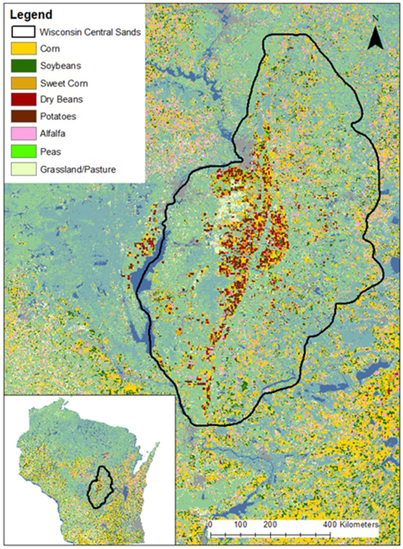
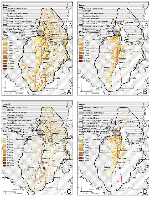
3.1. Crop Type Spatial Distributions, Area, and Frequency

In the WCS, 40.2% of the total land area (285,300 ha of 708,200 ha) was in agricultural use. On average, from 2008 to 2019 the eight crops reported in

Table 1. Total number of hectares for the eight main crop categories grown in the WCS from 2008 to 2019, their average hectare totals for each year, and standard deviations. In 2017 and 2018, sweet corn was misclassified in the USDA CDL as part of the corn category. The table reflects adjusted values for sweet corn and corn in each of those years (denoted with an asterisk), where the sweet corn annual average number of hectares for all other years (2008–2016, 2019) was used as a substitute in 2017–2018, and that value was subtracted from the corn category.

Year	Corn	Alfalfa	Soybean	Sweet Corn	Potato	Beans	Cereal	Peas	Total
Hectares
2008	65,233	32,483	18,948	22,787	17,864	13,819	10,789	3788	185,711
2009	63,514	31,493	19,222	26,186	17,303	12,008	28,316	2909	200,950
2010	67,505	20,904	19,538	22,059	18,192	14,247	5476	3223	171,144
2011	75,228	22,706	20,308	19,603	18,146	12,411	4883	2860	176,144
2012	82,399	21,324	20,450	21,948	20,627	8309	2916	2020	179,993
2013	85,403	22,579	15,442	18,818	17,719	12,089	9925	3228	185,203
2014	74,858	24,738	22,927	19,510	18,316	17,347	11,727	4297	193,721
2015	68,212	24,480	24,722	17,053	18,078	11,519	8406	5442	177,912
2016	75,548	19,029	21,891	25,143	18,860	11,822	8507	4412	185,214
2017	60,439*	17,517	27,401	20,915*	19,141	12,199	6909	4143	168,664
2018	60,893*	21,685	28,742	20,915*	18,046	13,578	6644	4706	175,209
2019	68,158	22,551	23,631	16,045	18,715	14,219	5023	5275	173,617
Average	70,616	23,457	23,457	20,915	18,417	12,797	9127	3859	181,123
St Dev	8091	4472	3777	3304	859	2150	6586	1040	9481

account for 64% of the agricultural land in the region. Distribution is greatly influenced by the five ecological landscapes that make up the region: Central Sand Hills, Central Sand Plains, Forest Transition, Central Lake Michigan Coastal, and Southeast Glacial Plains. The spatial distribution of several of the most dominant individual crop types (corn, potato, sweet corn, and alfalfa) in the WCS and their planting frequency during the 2008–2019 period are shown in Figure 2. Corn, soybean, cereal, and alfalfa were the only crops that are found throughout all five ecological landscapes. Potato, sweet corn, beans, and peas are found concentrated in Central Sand Plains, Central Sand Hills, and Forest Transition (Figure 2).

Corn was planted at least one time during the study period on 190,189 hectares, or 66.7% of agricultural land in the WCS, and had an annual average of 70,616 ha (24.8% of total agricultural land) (

Table 2. The dominant crops found in the Central Sands and their respective mean hectares and percent coverage of agricultural land. Standard deviation indicates the extent of deviation from the mean each rotation has; the CV is the coefficient of variation of annual average variability across all years; the slope, R², and p-value are from linear regression and indicate the change in hectares planted during the study period, how well this change represents the data, and whether this change is significant.

Crop	Mean Hectare	% Ag Land	St Dev	CV	Slope	R2	p-value
Corn	70,616	24.8%	35,482.9	1.9901	−323.0	0.0207	0.6554
Alfalfa	23,457	8.2%	11,380.8	2.0611	−797.1	0.4131	0.0242
Soybean	21,935	7.7%	10,504.9	2.0881	770.8	0.5416	0.0064
Sweet Corn	20,915	7.3%	9872.9	2.1184	−405.2	0.2390	0.1068
Potato	18,417	6.5%	8399.3	2.1927	67.2	0.7950	0.3746
Beans	12,797	4.5%	5705.0	2.2432	56.4	0.0090	0.7699
Cereal	9127	3.2%	5826.3	1.5665	−741.5	0.1648	0.0106
Peas	3859	1.4%	1185.5	3.2549	203	0.4955	0.1905
Total	181,123	63.5%

). One percent of agricultural land (2025 ha) was planted with continuous corn. Corn was found in all five ecological landscapes, with 75% occurring between Central Sand Plains and Central Sand Hills regions. Common frequencies range from three to eight years in all regions except for Central Sand Plains which has the highest amount of land with corn only grown once during the study period (16,336 ha or 24% of corn grown in the region). Sweet corn was planted at least one time on 78,482 hectares or 27.7% of agricultural land, with an average of 20,915 ha planted annually or 7.3% of all agricultural land (Table 2). Sweet corn is found in three ecological landscapes, with 70.9% (40,536 ha) of all sweet corn grown in the Central Sand Plains. Individual land unit frequencies are as high as nine total years (frequency totals were not adjusted for missing acres) but are commonly between one through four years. Potato was planted at least once on 66,257 hectares, or 23.4% of agricultural land, with 72.4% (47,988 ha) occurring in the Central Sand Plains. Potato was also grown in the Central Sand Hills (22.2% of total potato plantings, 14,679 ha) and Forest Transition (5.4%, 3556 ha). Potato is annually planted on only 6.5% (18,417 ha) of agricultural land in the WCS (Table 2). Fields that are in potato commonly return between one through four years during the study period, with less than 1% returning seven out of the twelve years. Alfalfa was planted at least once on 62,772 hectares, or 22.2% of agricultural land, and has an annual average of 23,457 ha (or 8.2% of agricultural land) (Table 2). Alfalfa is found throughout all five ecological landscapes and has the most hectares planted in the Central Sand Hills (27,660 ha). Frequency values most commonly range from one to six years with 1.4% in continuous alfalfa. While soybean is not shown in Figure 2, it is most often grown in rotation with corn and was planted at least once on 101,717 ha (35.7% of agricultural land), with an annual average of 21,935 ha (or 7.7% of agricultural land) (Table 2). Soybean frequencies are most common between one and four years (out of twelve years), with 34.5% grown only once during the study period.

A concentrated area of agricultural land is found within 10 km to either side of the Central Sand Plains and the Central Sand Hills ecological boundaries. Ninety-four percent of potato plantings are found within Central Sand Plains and Central Sand Hills, with 73.1% of that occurring within this boundary. Sweet corn, beans, and peas also have a strong presence within this boundary, accounting for 75.6%, 75.3%, and 73.3% of plantings, respectively. Corn, soybean, alfalfa, and cereal are also planted but account for 47.1%, 40.2%, 36.3%, and 33.3% of plantings, respectively.

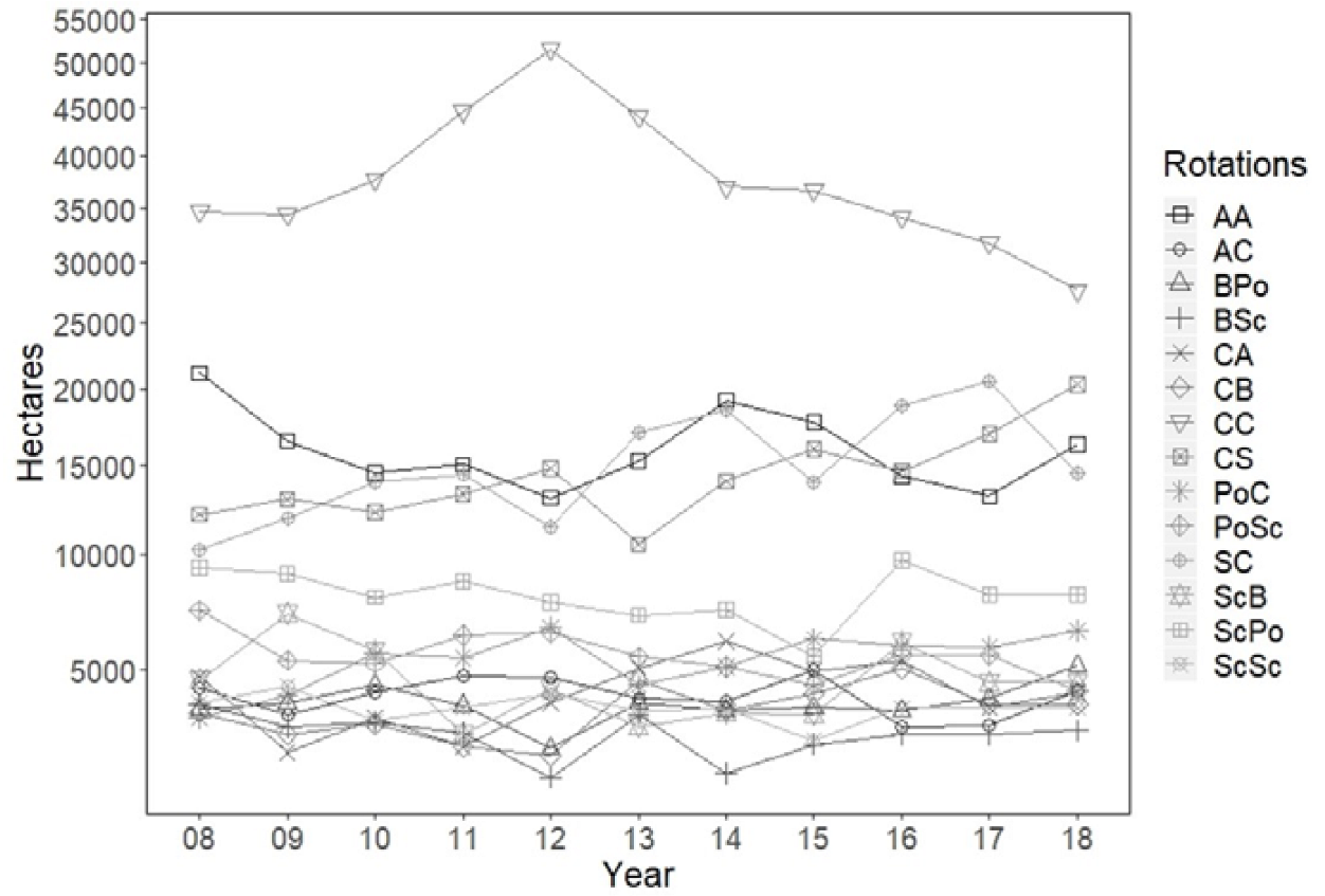
3.2. Common Two- and Three-Year Rotations

Two- and three-year rotations were determined for the eight crops and the other crops category and were compared using their annual average land area totals over the study period. Fourteen dominant two-year rotations were identified to occur on 130,801 hectares each year, or 45.9% of WCS agricultural land (

Table 3. Most common two-year rotations and their respective average hectare totals and percent coverage of agricultural land in the WCS. Standard deviation indicates the extent of deviation from the mean each rotation has; the CV is the coefficient of variation of annual average variability across all years; the slope, R², and p-value are from linear regression and indicate the change in hectares planted during the study period, how well this change represents the data, and whether this change is significant. The following abbreviations correspond to the crop grown; C = corn, A = alfalfa, S = soybean, Sc = sweet corn, Po = potato, B = beans.

Rotations	Mean Hectare	% Ag Land	St Dev	CV	Slope	R2	p-Value
CC	37,673	13.2%	6720.4	0.1784	−791.2	0.1525	0.2351
AA	16,014	5.6%	2541.2	0.1587	−246.8	0.1037	0.3341
SC	15,031	5.3%	3340.2	0.2222	703.5	0.4880	0.0168
CS	14,346	5.0%	2714.9	0.1892	630.4	0.5931	0.0056
ScPo	8062	2.8%	1159.0	0.1438	−105.7	0.0915	0.3659
PoSc	5580	2.0%	878.8	0.1575	−169.2	0.4078	0.0344
PoC	5405	1.9%	1014.9	0.1878	210.98	0.4754	0.0189
ScSc	5160	1.8%	419.9	0.0814	−44.31	0.1225	0.2913
ScB	4599	1.6%	1298.7	0.2823	−86.42	0.0487	0.5143
CA	4263	1.5%	1127.3	0.2644	134.9	0.1576	0.2267
AC	4137	1.5%	614.6	0.1485	−45.54	0.0604	0.4664
BPo	3891	1.4%	618.7	0.1590	57.43	0.0948	0.3570
CB	3663	1.3%	800.9	0.2186	130.22	0.2908	0.0869
BSc	2970	1.0%	588.4	0.1981	−57.82	0.1062	0.3281
Total	130,801	45.9%

). Continuous corn was the most common two-year rotation, which occurred on 13.2% of agricultural land (Table 3). Other dominant two-year rotations included alfalfa–alfalfa (5.6%), soy–corn (5.3%), corn–soy (5.0%), and sweet corn–potato (2.8%) (Table 3). Continuous corn reached a max imum extent of 51,514 ha in 2012 and then steadily decreased thereafter (Figure 3). The two-year rotation of continuous alfalfa declined at the same time continuous corn and corn–soy were increasing, suggesting that corn and soy were replacing alfalfa in some of these rotations (Figure 3). At the time that continuous corn was declining after 2012, corn–soy and soy–corn exhibited a steady increase in planted area (Figure 3). The increases in corn–soy and soy–corn were significant (p < 0.05) across the entire study period (Table 3). There was also a significant increase in potato–corn rotations (p = 0.019) and a significant decline in potato–sweet corn (p = 0.034) during the study period. The remaining two-year rotations remained relatively consistent during the study period with no significant trends.

We identified sixteen three-year rotations that were found on 98,481 ha, or 31.4% of agricultural land in the WCS (

Table 4. Most common three-year rotations and their respective average hectare totals and percent coverage of agricultural land in the WCS. Standard deviation indicates the extent of deviation from the mean each rotation has; the CV is the coefficient of variation of annual average variability across all years; the slope, R², and p-value are from linear regression and indicate the change in hectares planted during the study period, how well this change represents the data, and whether this change is significant. The following abbreviations correspond to the crop grown; C = corn, A = alfalfa, S = soybean, Sc = sweet corn, Po = potato, B = beans.

Rotations	Mean Hectare	% Ag Land	St Dev	CV	Slope	R2	p-Value
CCC	24,329	8.5%	4076.3	0.1675	−545.8	0.1643	0.2451
CSC	11,410	4.0%	2184.4	0.1914	527.1	0.5337	0.0164
AAA	11,334	4.0%	1818.3	0.1604	23.0	0.0015	0.9165
CCS	6638	2.3%	2036.3	0.3067	150.0	0.0498	0.5356
SCS	6602	2.3%	1426.4	0.2161	386.7	0.6739	0.0036
SCC	5119	1.8%	1230.0	0.2403	15.7	0.0015	0.9157
CAA	3259	1.1%	925.0	0.2838	181.0	0.3509	0.0712
AAC	3245	1.1%	514.6	0.1586	−36.0	0.0449	0.5566
ACC	2929	1.0%	547.8	0.1870	−98.6	0.2968	0.1034
CCA	2874	1.0%	832.6	0.2897	139.0	0.2554	0.1362
ScPoSc	2749	1.0%	369.6	0.1345	−60.9	0.2492	0.1419
ScBPo	2050	0.7%	712.9	0.3477	−98.9	0.1764	0.2269
ScScPo	1847	0.6%	315.4	0.1708	−48.5	0.2167	0.1752
ScPoB	1756	0.6%	586.7	0.3341	−7.3	0.0014	0.9174
PoBC	1690	0.6%	1316.4	0.7791	306.9	0.4982	0.0226
PoCB	1650	0.6%	861.1	0.5218	255.1	0.8047	0.0004
Total	89,481	31.4%

). Continuous corn was the most common three-year rotation (8.5%), followed by continuous alfalfa (4.0%) and various combinations of corn and soy including corn–soy–corn (4.0%), corn–corn–soy (2.3%), soy–corn–soy (2.3%), and soy–corn–corn (1.8%). Continuous corn reached a peak in 2011 of 31,298 ha and then exhibited a long-term decreasing trend through 2017 (Figure 4). Corn–soy–corn and soy–corn–soy rotations exhibited a significant increasing trend through the period (p < 0.05; Table 4). Two of the three-year rotations including potato–beans–corn and potato–corn–beans exhibited significant increases in area during the study period (p < 0.05; Table 4). None of the other dominant three-year rotations showed significant trends from 2008 to 2019 (Table 4).

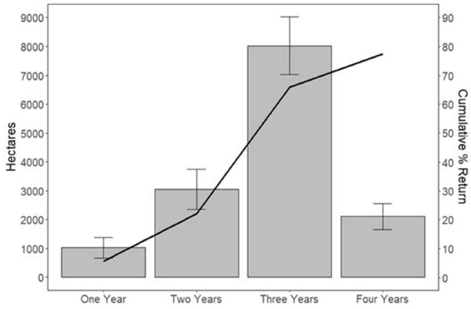
3.3. Return Time to Potato and Most Common Rotations

The analysis of multiyear rotations that began and ended with potato show that on average 5.6% (1025 ha) of potato returned to potato immediately, 16.6% (3050 ha) returned the second year after initial planting, 43.7% (8072 ha) returned in the third year, and 11.6% (2109 ha) returned after four years (Figure 5). This suggests that the most popular year in a potato rotation to come back to potato is year three (two years after the initial planting). A total of 64.8% and 77.4% of fields planted with potato have returned to that crop by the fourth and fifth years in the rotation, respectively (three- and four-year gaps, respectively) (Figure 5). The most common crops that are rotated with potato include sweet corn, corn, and beans. Sweet corn most commonly is grown between potato plantings, accounting for 47.5% of all two-year rotations, followed by corn (17.5%), and beans (15.8%) (

Table 5. Common rotations when rotating with potato after two- (one year off potato), three- (two years off potato), and four-years (three years off potato), mean number of hectares that rotation would occur, and the percent weight compared to all other two-, three-, and four-year potato rotations. Standard deviation indicates the extent of deviation from the mean each rotation has; the CV is the coefficient of variation of annual average variability across all years; the slope, r2 and p-value are from linear regression and indicates the change in hectares planted during the study period, how well this change represents the data, and whether this change is significant. The following abbreviations correspond to the crop grown; C = corn, Sc = sweet corn, Po = potato, B = beans.

Rotation	Mean Hectare	% One Year Off	St dev	CV	Slope	R2	p-Value
PoScPo	1450	47.5%	445.8	0.3074	−69.3	0.2215	0.1698
PoCPo	534	17.5%	171.0	0.3203	−10.6	0.0352	0.6035
PoBPo	481	15.8%	163.4	0.3398	−11.8	0.0475	0.5455
Total	2465	80.8%
Rotation	Mean Hectare	% Two Years Off	St dev	CV	Slope	R2	p-value
PoScScPo	1017	12.7%	535.6	1.8996	−34.7	0.2733	0.1487
PoScBPo	865	10.8%	465.3	1.8596	−40.5	0.2811	0.1420
PoBScPo	854	10.7%	465.2	1.8366	−23.8	0.0788	0.4643
PoCBPo	810	10.1%	560.3	1.4458	135.3	0.4537	0.0467
Total	3547	44.2%
Rotation	Mean Hectare	% Three Years Off	St dev	CV	Slope	R2	p-value
PoScBScPo	342	16.2%	190.5	1.7965	21.9	0.2294	0.2298
PoBScBPo	148	7.0%	108.6	1.3606	−22.3	0.2213	0.2395
PoCCBPo	126	6.0%	86.4	1.4562	16.4	0.2120	0.2509
Total	616	29.2%

). Rotations with two years of sweet corn grown in between potato crops account for 12.7% of all three-year rotations, and combinations of beans and sweet corn comprise 21.5% (Table 5). The cropping sequences that are most frequently found in four-year potato rotations include sweet corn–beans–sweet corn (16.2%), beans–sweet corn–beans (7.0%), and corn–corn–beans (6.0%) (Table 5). Only one potato rotation (potato–corn–beans–potato) exhibited a significant trend (increasing area; p = 0.047) over the study period (Table 5).

4. Discussion

4.1. Spatial Distribution and Frequency of Common Crops Grown in the WCS Is Dictated by Soil Formation Processes

The five ecological landscapes that are located within the WCS (Central Sand Hills, Central Sand Plains, Forest Transition, Central Lake Michigan Coastal, and Southeast Glacial Plains) have landforms left behind by glacial activity that influence spatial distribution of agricultural production. Over 24,000 years ago, the Green Bay Lobe ice sheet entered the WCS from the east and reached its maximum extent between the Central Sand Hills and Central Sand Plains ecological landscapes, creating series of moraines and leaving glacial outwash behind as it advanced and retreated before fully retreating from the area over 12,000 years ago [7]. The outermost moraine is known as the Johnstown Moraine and is exemplified by low hills that run north and south along the border of these two ecological landscapes and into Forest Transition [7]. About 19,000 years ago, the Green Bay Lobe advanced into and blocked the ancient river now known as the Wisconsin River, creating Glacial Lake Wisconsin within the Central Sand Plains [37]. Layers of silt were deposited on the lakebed and then covered with sand, leading to poor drainage and wetlands throughout this region when the glacial lake was drained. The eastern part of the Wisconsin Sand Plains near the Johnstown Moraine has outwash sand deposits that are thicker and higher above the water table, allowing for soils to be drained enough to grow vegetable crops with the use of irrigation [37]. The spatial distribution east of the Johnstown Moraine is influenced by the location of moraines and glacial outwash left between them after the glacier fully retreated. Deposits range from poorly to excessively well drained, making agricultural production dependent on irrigation and drainage [7,37,38,39,40].

4.2. A High Number of Growers Use Multiple Year Rotations with Potato, but a Significant Fraction Return to Potato Immediately or by the Third Year

Potato is a high-value crop and a major component to the WCS’s economy, contributing USD 522 million to Wisconsin’s economy annually [41], thereby creating incentives for farmers to keep it in rotation. However, potatoes require large quantities of water and nutrients in a region that is susceptible to leaching or fertilizer, which has contributed to the region’s groundwater quality issues [42]. Finding a balance between economic return and environmental sustainability is needed to keep the region profitable and reduce impacts on land and water resources. Implementing a diverse crop rotation for high-value potato can be beneficial in replenishing soil nutrients and decrease the likelihood of disease and weed persistence [4], but also can be economically beneficial. According to Halloran et al. [43], there are three sources of potential economic benefits to crop rotations: the rotation either increases yields of the target crop (potato) at current or reduced input levels, the rotation crop itself is profitable, and the economic risk is reduced by income variability. In Halloran et al. [43], barley, sweet corn, green bean, soybean, canola, and continuous potato were simulated as two-year rotation sequences to estimate the expected mean net income and income variability. Potato–potato, green bean–potato, and sweet corn–potato rotations were found to be most profitable due to high-valued commodities. However, economic risk associated with potato–potato is high due to a loss in diversity, whereas the economic risk with green bean–potato is low, although a decline in potato yield was found the year following green bean from an increase in powdery mildew. In another study by Watkins et al. [44], they used the EPIC model to study two-, three-, and four-year rotations and their economic impact and environmental outcomes for seed potatoes in Idaho. A three-year rotation of potatoes followed by two grain crops of either spring wheat, barley, oats, and canola (potato–grain crop–grain crop) was found to have reduced nitrogen loss and soil erosion and obtained the most economic return.

These studies generally reflect recommended best practices for potato to spend two or more years out of rotation before returning to potato and to include snap beans, peas, sweet corn, field corn, small grains, and alfalfa [10]. In the Wisconsin Central Sands, these rotation recommendations with potato were generally observed, with 44% of fields returning to potato after three years off, and that sweet corn, corn, and beans are the most frequently rotated crops. Beans, potato, and sweet corn come from different plant families and differ in term of disease and insect host, making this combination an environmentally sustainable rotation [10]. Although most fields are implementing rotations, there were still a significant fraction of fields that returned to potato immediately in the following year or after only one year of an alternate crop planting. Rowberry et al. [45] compared profitability between a seven-year rotation of barley, corn, soybean, and potato to a rotation of continuous potato and found the continuous potatoes to be more profitable with a slight decline in yield. Some producers in the WCS region might be sacrificing yield, reduced soil health, and increased input costs to continually produce a higher-valued crop each year. Furthermore, given the high amounts of nitrogen fertilizer required for potato in the WCS, this may be exacerbating the ongoing water quality issues. However, the most common rotation of potato in the WCS is where two years of other crops are planted in between potato crops.

4.3. Changes in Continuous Corn Area and Increase in Soybean Reflect Changes in Energy Policy and Market Prices

The overall trend of declining continuous corn area after 2012 coupled with increases in soybean in rotation are reflective of changes in markets and prices and a push towards more sustainable management practices in the Midwest U.S. that lead to improved soil and water health. The desire for cleaner fuels and reduced greenhouse gas emissions have led to changes in policy and standards for biofuels [46], which has impacted land use change in agricultural landscapes such as the Wisconsin Central Sands. In the Energy Policy Act of 2005, the Renewable Fuel Standard (RFS) was established, requiring fuel to contain specific amounts of ethanol and the 2008 Farm Bill promoted the processing and production of this ethanol through subsidies [47,48]. In the years following, corn and soybean saw an intensification in acres planted in the United States coming from a reduction in pasture, CRP enrollment, and cropland expansion on land typically deemed not suitable for row crop production [35]. From 2009 to 2013 in the WCS, continuous corn area sharply increased until it reached a peak in 2012 before decreasing thereafter. Countering this rise, hectares planted in cereals and beans declined during these years. The rise and fall of the amount of continuous corn grown also reflects a pattern of changing corn prices. In August 2012, a drought impacted much of the corn belt and caused corn prices to reach a maximum of USD 8.24/bushel [49]. At the beginning of 2013, corn prices were forecasted to be within USD 6.95–8.25/bushel, likely causing the spike in corn hectares planted within the WCS [50]. During the 2013 growing season, the price of corn started to drop and was likely a major factor in the decline of corn planted in years following.

Common rotations with corn in the WCS region include soybean and alfalfa, with significant increases in those rotations that include corn and soybean during the study period. Soybean is a desired crop due to its high economic value and its ability to fix nitrogen from the atmosphere through determinate nodules in its root system which can be used by the plant as well as replenishing the soil nitrogen content after the plant dies and decomposes [51]. Adding soybean to a rotation can increase crop yield and enhance soil fertility, while reducing the need for additional sources of nitrogen [52,53,54]. These are particularly important for a region such as the WCS with its sandy soils and generally lower organic matter content. Alfalfa is commonly left in rotation for several years, allowing roots to penetrate deeper, improving soil structure and increasing organic matter. Rotating alfalfa with corn or other small grains has been found to be more profitable for farmers. Younger alfalfa stands (three years and younger) provide a higher yield than older stands and provide a boost in corn yield the year following alfalfa by 10% compared to corn following corn [55].

5. Conclusions

The WCS is a very diverse and important agricultural region that is faced with challenges of growing high-value crops on soils with low nutrient and water holding capacities. By implementing best management practices through more precise fertilizer applications, deficit irrigation, and crop rotations, the region can address some of the current environmental challenges around water resources facing the region. For this study, we looked at the spatial distribution of the dominant crops, common rotation combinations, and the amount of land area in each of these, the typical time between consecutive potato plantings, and agricultural land use trends during the 2008–2019 time period.

The spatial distribution and frequency of crops grown within the region is partially influenced by the ecological landscapes and soil formations within them left from the last glaciation from 12,000 years ago. The Johnstown Moraine, which roughly divides the WCS north to south, marks the furthest extent of the Green Bay Lobe which carved moraines and deposited glacial outwash as it advanced and retreated in the area [7]. Outwash deposits left between moraines range from poorly to excessively well drained and depth to water table influences the spatial distribution of agricultural land in the WCS. High frequencies of plantings are observed out to twelve years for potato, corn, alfalfa, and beans, but due to the diverseness of the region, continuous cropping is not commonly observed.

Corn is the most planted crop in the region and covers on average 24.8% of agricultural land each year. We defined thirteen two-year and sixteen three-year rotation combinations that cover 45.9% and 31.4% of agricultural land each year. These rotations include corn, soybean, sweet corn, potato, alfalfa, and beans. Continuous corn was the most dominant rotation followed by continuous alfalfa and corn–soy combinations for both two- and three-year rotation combinations. The amount of agricultural land in the WCS planted in continuous corn has declined since 2012, whereas there has been a significant increase in soybean planted in rotation with corn since 2008.

A majority of producers are following recommended management practices to reduce disease and weed pressure by introducing two or more annual crops into potato rotations; 16.6% of fields growing potato return to that crop after two years, with an additional 43.7% of fields returning to potato after three years off. On average each year, 5.6% of fields with potato are planted with that crop continuously. We suspect a key reason for growers to not exercise longer 4- and 5-year rotations for potato is the high value of the crop; this likely contributes to a significant fraction of producers to keep potato in continuous rotation (or return after only one year off), but this comes with the increased risk of disease and lower yields on average.

Given the N fertilizer requirements of potato and ongoing water quality issues in the WCS, where a significant fraction of private wells are greater than the EPA safe drinking water standard threshold of 10ppm [56], rotating crops with potato that require zero or less inorganic N fertilizer, and extending all potato rotations to at least 4 or 5 years could be a management option that helps to reduce nitrate leaching to groundwater in the long term.

References

1. Laboski, C.A.M.; Peters, J.B. Nutrient Application Guidelines for Field, Vegetable, and Fruit Crops in Wisconsin Nutrient Application Guidelines for Field, Vegetable, and Fruit Crops in Wisconsin. 2012. Available online: http://corn.agronomy.wisc.edu/management/pdfs/a2809.pdf (accessed on 3 December 2021).
2. Prunty, L.; Greenland, R. Nitrate leaching using two potato-corn N-fertilizer plans on sandy soil. Agric. Ecosyst. Environ. 1997, 65, 1–13. [Google Scholar] [CrossRef]
3. Larkin, R.P.; Honeycutt, C.W.; Olanya, O.M.; Halloran, J.M.; He, Z. Impacts of Crop Rotation and Irrigation on Soilborne Diseases and Soil Microbial Communities. In Sustainable Potato Production: Global Case Studies; Springer: Berlin/Heidelberg, Germany, 2012; pp. 23–41. [Google Scholar] [CrossRef]
4. Larkin, R.P. Crop Rotation and Soil Health in Potato Production Systems. Grow Plant Health Exch. 2019. [Google Scholar] [CrossRef]
5. NASS. Vegetables 2019 Summary; USDA: Washington, DC, USA, 2020; pp. 1–101. [Google Scholar]
6. Kraft, G.J.; Clancy, K.; Mechenich, D.J.; Haucke, J. Irrigation Effects in the Northern Lake States: Wisconsin Central Sands Revisited. Ground Water 2012, 50, 308–318. [Google Scholar] [CrossRef] [PubMed]
7. Wisconsin Department of Natural Resources. The Ecological Landscapes of Wisconsin: An Assessment of Ecological Resources and a Guide to Planning Sustainable Management. In Central Sand Hills Ecological Landscape; Chapter 9; Wisconsin Department of Natural Resources: Madison, WI, USA, 2015. [Google Scholar]
8. Kniffin, M.; Potter, K.; Bussan, A.; Colquhoun, J.; Bradbury, K. Sustaining Central Sands Water Resources: State of the Science. Master’s Thesis, University of Wisconsin-Madison, Madison, WI, USA, 2014; pp. 1–100. [Google Scholar]
9. Kraft, G.J.; Mechenich, D.J.; Haucke, J. Information Support for Groundwater Management in the Wisconsin Central Sands, 2011–2013; Wisconsin Department of Natural Resources: Madison, WI, USA, 2014. [Google Scholar]
10. Knuteson, D.L.; Groves, R.L.; Colquhoun, J.B.; Ruark, M.; Gevens, A.J.; Bussan, A.J. BioIPM Potato Workbook. Lit. Imagin. 2003, 5, 179. [Google Scholar] [CrossRef]
11. Emmond, G.S.; Ledingham, R.J. Effects of crop rotation on some soil-borne pathogens of potato. Can. J. Plant Sci. 1972, 52, 605–611. [Google Scholar] [CrossRef] [Green Version]
12. Frank, J.A.; Murphy, H.J. The effect of crop rotations on rhizoctonia disease of potatoes. Am. Potato J. 1977, 7, 541–559. [Google Scholar] [CrossRef]
13. Pedersen, E.A.; Hughes, G.R. The Effect of Crop Rotation on Development of the Septoria Disease Complex on Spring Wheat in Saskatchewan. Can. J. Plant Pathol. 1992, 14, 152–158. [Google Scholar] [CrossRef]
14. Scholte, K. The effect of crop rotation and granular nematicides on the incidence of Rhizoctonia solani in potato. Potato Res. 1987, 30, 187–199. [Google Scholar] [CrossRef]
15. Huber, D.M.; Watson, R.D.; Steiner, G.W. Crop Residues, Nitrogen, and Plant Disease. Soil Sci. 1965, 100, 302–308. [Google Scholar] [CrossRef]
16. Fry, W.E. Disease Management in Practice. Princ. Plant Dis. Manag. 1982, 303–329. [Google Scholar] [CrossRef]
17. Bélair, G.; Dauphinais, N.; Fournier, Y.; Dangi, O.P.; Ciotola, M. Canadian Journal of Plant Pathology Effect of 3-year rotation sequences and pearl millet on population densities of Pratylenchus penetrans and subsequent potato yield. Can. J. Plant Pathol. 2006, 28, 230–235. [Google Scholar] [CrossRef]
18. Rupp, J.; Jacobsen, B. Bacterial and Fungal Disease of Potato and Their Management; Montana State University Extension: Bozeman, MT, USA, 2017. [Google Scholar]
19. Sill, W.H.J. Plant Protection, an Integrated Interdisciplinary Approach; Iowa State University Press: Ames, IA, USA, 1982. [Google Scholar]
20. Honeycutt, C.W.; Clapham, W.M.; Leach, S.S. Crop rotation and N fertilization effects on growth, yield, and disease incidence in potato. Am. Potato J. 1996, 73, 45–61. [Google Scholar] [CrossRef]
21. Peters, R.D.; Sturz, A.V.; Carter, M.R.; Sanderson, J.B. Developing disease-suppressive soils through crop rotation and tillage management practices. Soil Tillage Res. 2003, 72, 181–192. [Google Scholar] [CrossRef]
22. Williams, L.E.; Schmitthenner, A.F. Effect of crop rotations on soil fungus populations. Phytopathology 1962, 52, 241–247. [Google Scholar]
23. Peters, R.D.; Sturz, A.V.; Carter, M.R.; Sanderson, J.B. Influence of crop rotation and conservation tillage practices on the severity of soil-borne potato diseases in temperate humid agriculture. Can. J. Soil Sci. 2004, 84, 397–402. [Google Scholar] [CrossRef]
24. Azzari, G.; Grassini, P.; Edreira, J.I.R.; Conley, S.; Mourtzinis, S.; Lobell, D.B. Satellite mapping of tillage practices in the North Central US region from 2005 to 2016. Remote Sens. Environ. 2019, 221, 417–429. [Google Scholar] [CrossRef]
25. Noe, R.R. Uncertainty in Cropland Data Layer derived Land-Use Change Estimates: Putting Corn and Soy Expansion Estimates in Context. Master’s Thesis, University of Minnesota, Minneapolis, MN, USA, 2015. [Google Scholar]
26. Yost, M.A.; Russelle, M.P.; Coulter, J.A.; Bolstad, P.V. Alfalfa Stand Length and Subsequent Crop Patterns in the Upper Midwestern United States. Agron. J. 2014, 106, 1697–1708. [Google Scholar] [CrossRef]
27. Stern, A.J.; Doraiswamy, P.C.; Raymond Hunt, E. Changes of crop rotation in Iowa determined from the United States Department of Agriculture, National Agricultural Statistics Service cropland data layer product. J. Appl. Remote Sens. 2012, 6, 063590. [Google Scholar] [CrossRef]
28. Long, J.A.; Lawrence, R.L.; Miller, P.R.; Marshall, L.A. Changes in field-level cropping sequences: Indicators of shifting agricultural practices. Agric. Ecosyst. Environ. 2014, 189, 11–20. [Google Scholar] [CrossRef]
29. Lark, T.J.; Mueller, R.M.; Johnson, D.M.; Gibbs, H.K. Measuring land-use and land-cover change using the U.S. department of agriculture’s cropland data layer: Cautions and recommendations. Int. J. Appl. Earth Obs. Geoinf. 2017, 62, 224–235. [Google Scholar] [CrossRef]
30. Johnston, C.A. Agricultural expansion: Land use shell game in the U.S. Northern Plains. Landsc. Ecol. 2014, 29, 81–95. [Google Scholar] [CrossRef]
31. USDA-NASS. USDA—National Agricultural Statistics Service—Research and Science-CropScape and Cropland Data Layer-Announcements 2021. Available online: https://www.nass.usda.gov/Research_and_Science/Cropland/SARS1a.php (accessed on 22 June 2021).
32. Wisconsin DNR. Central Sands Background and Outreach Resources. 2021. Available online: https://dnr.wisconsin.gov/topic/Wells/HighCap/CSLBackground.html (accessed on 2 August 2021).
33. ESRI. ArcGIS Desktop: Release 10.7.1; ESRI: Redlands, CA, USA, 2019. [Google Scholar]
34. Hennessy, D. On Monoculture and the Structure of Crop Rotations. Am. J. Agric. Econ. 2006, 88, 900–914. [Google Scholar] [CrossRef] [Green Version]
35. Lark, T.J.; Meghan Salmon, J.; Gibbs, H.K. Cropland expansion outpaces agricultural and biofuel policies in the United States. Environ. Res. Lett. 2015, 10, 44003. [Google Scholar] [CrossRef] [Green Version]
36. Wisconsin Department of Natural Resources. The Ecological Landscapes of Wisconsin: An Assessment of Ecological Resources and a Guide to Planning Sustainable Management; Wisconsin Department of Natural Resources: Madison, WI, USA, 2015. [Google Scholar]
37. Wisconsin Department of Natural Resources. The ecological landscapes of Wisconsin: An assessment of ecological resources and a guide to planning sustainable management. In Central Sand Plains Ecological Landscape; Chapter 10; Wisconsin Department of Natural Resources: Madison, WI, USA, 2015. [Google Scholar]
38. Wisconsin Department of Natural Resources. The ecological landscapes of Wisconsin: An assessment of ecological resources and a guide to planning sustainable management. In Forest Transition Ecological Landscape; Chapter 11; Wisconsin Department of Natural Resources: Madison, WI, USA, 2015. [Google Scholar]
39. Wisconsin Department of Natural Resources. The ecological landscapes of Wisconsin: An assessment of ecological resources and a guide to planning sustainable management. In Southeast Glacial Plains Ecological Landscape; Chapter 18; Wisconsin Department of Natural Resources: Madison, WI, USA, 2015. [Google Scholar]
40. Wisconsin Department of Natural Resources. The ecological landscapes of Wisconsin: An assessment of ecological resources and a guide to planning sustainable management. In Central Lake Michigan Coastal Ecological Landscape; Chapter 8; Wisconsin Department of Natural Resources: Madison, WI, USA, 2015. [Google Scholar]
41. Kashian, R.; Depas, J.; Fogarty, P.; Peterson, J. Potato Production in Wisconsin: Analyzing the Economic Impact; University of Wisconsin-Whitewater: Whitewater, WI, USA, 2014. [Google Scholar]
42. Kraft, G.J.; Browne, B.A.; Devita, W.M.; Mechenich, D.J. Nitrate and Pesticide Residue Penetration into a Wisconsin Central Sand Plain Aquifer; University of Wisconsin-Stevens Point: Stevens Point, WI, USA, 2004. [Google Scholar]
43. Halloran, J.M.; Griffin, T.S.; Honeycutt, C.W. An economic analysis of potential rotation crops for Maine Potato cropping systems. Am. J. Potato Res. 2005, 82, 155–162. [Google Scholar] [CrossRef]
44. Watkins, K.B.; Lu, Y.-C. Economic and environmental tradeoffs among alternative seed potato rotations. J. Sustain. Agric. 1998, 13, 37–53. [Google Scholar] [CrossRef]
45. Rowberry, R.; Anderson, G. The profitability of continuous potatoes versus rotations including potatoes and other cash crops. Am. Potato J. 1983, 60, 503–510. [Google Scholar] [CrossRef]
46. Li, R.; Monti, A. Land Allocation for Biomass Crops: Challenges and Opportunities with Changing Land Use; Springer International Publishing: Berlin/Heidelberg, Germany, 2018. [Google Scholar] [CrossRef]
47. Lewandrowski, J.; Rosenfeld, J.; Pape, D.; Hendrickson, T.; Jaglo, K.; Moffroid, K. The greenhouse gas benefits of corn etha-nol-assessing recent evidence. Biofuels 2020, 11, 361–375. [Google Scholar] [CrossRef] [Green Version]
48. CRS Report for Congress Biofuels Provisions in the 2007 Energy Bill and the 2008 Farm Bill: A Side-by-Side Comparison-name redacted-Specialist in Agricultural Policy-name redacted-Specialist in Energy and Environmental Policy. 2009. Available online: https://www.everycrsreport.com/reports/RL34239.html (accessed on 6 January 2021).
49. Mallya, G.; Zhao, L.; Song, X.C.; Niyogi, D.; Govindaraju, R.S. 2012 Midwest Drought in the United States. J. Hydrol. Eng. 2013, 18, 737–745. [Google Scholar] [CrossRef]
50. USDA-ERS. USDA ERS—U.S. Drought 2012: Farm and Food Impacts; USDA-ERS: Washington, DC, USA, 2015. [Google Scholar]
51. Ferguson, B.J.; Indrasumunar, A.; Hayashi, S.; Lin, M.H.; Lin, Y.H.; Reid, D.E.; Gresshoff, P.M. Molecular analysis of legume nodule development and autoregulation. J. Integr. Plant Biol. 2010, 52, 61–76. [Google Scholar] [CrossRef]
52. Hirel, B.; le Gouis, J.; Ney, B.; Gallais, A. The challenge of improving nitrogen use efficiency in crop plants: Towards a more central role for genetic variability and quantitative genetics within integrated approaches. J. Exp. Bot. 2007, 58, 2369–2387. [Google Scholar] [CrossRef]
53. Peoples, M.B.; Brockwell, J.; Herridge, D.F.; Rochester, I.J.; Alves, B.J.R.; Urquiaga, S.; Boddey, R.M.; Dakora, F.D.; Bhattarai, S.; Maskey, S.L.; et al. The contributions of nitrogen-fixing crop legumes to the productivity of agricultural systems. Symbiosis 2009, 48, 1–17. [Google Scholar] [CrossRef]
54. Canfield, D.E.; Glazer, A.N.; Falkowski, P.G. The evolution and future of earth’s nitrogen cycle. Science 2010, 330, 192–196. [Google Scholar] [CrossRef] [PubMed] [Green Version]
55. Undersander, D.; Cosgrove, D.; Cullen, E.; Grau, C.; Rice, M.E.; Renz, M.; Sheaffer, C.; Shewmaker, G.; Sulc, M. Alfalfa Management Guide; American Society of Agronomy: Madison, WI, USA; Crop Science Society of America: Madison, WI, USA; Soil Science Society of America: Madison, WI, USA, 2011. [Google Scholar]
56. Center for Watershed Science and Education. WI Well Water Viewer. 2019. Available online: https://www.uwsp.edu/cnr-ap/watershed/Pages/WellWaterViewer.aspx (accessed on 14 September 2021).
Figure 1. The 2019 USDA Cropland Data Layer (CDL) and dominant crop types found in the Wisconsin Central Sands (dark black outline). This boundary is defined as a contiguous area east of the Wisconsin River with sand and gravel deposits greater than 50 feet deep (Wisconsin DNR).
Land 11 00273 g001
Figure 2. Frequency of crop plantings between 2008 and 2019 for (A) corn, (B) potato, (C) alfalfa, and (D) sweet corn. Sweet corn frequency totals were not adjusted for missing data in 2017 and 2018. The five ecological landscapes that are found within the WCS are shown.
Land 11 00273 g002
Figure 3. Dominant two-year rotations and their respective area totals for each year from 2008 to 2018. Total hectares on the Y axis are expressed with log scale. The following abbreviations correspond to the crop grown; C = corn, A = alfalfa, S = soybean, Sc = sweet corn, Po = potato, B = beans.
Land 11 00273 g003
Figure 4. Dominant three-year rotations and their respective area totals for each year from 2008 to 2017. Total hectares on the Y axis are expressed with log scale. The following abbreviations correspond to the crop grown; C = corn, A = alfalfa, S = soybean, Sc = sweet corn, Po = potato, B = beans.
Land 11 00273 g004
Figure 5. Bar graph represents the average hectares of potato that return after one year (continuous potato), two years (one crop between potato plantings), three years (two crops between), and four years (three crops between), and their respective standard deviations marked by error bars. The line graph represents the cumulative percent of the initial potato crop that has returned to potato.
Land 11 00273 g005