A New Perspective for Urban Development Boundary Delineation Based on the MCR Model and CA-Markov Model

Abstract

In order to control the development of urban space, it is important to explore scientific methods to provide a reference for regional territorial space planning. On the basis of the minimum cumulative resistance (MCR) model and the cellular automaton (CA)-Markov model, we constructed a new technical method for delineating urban development boundaries, exploring the temporal and spatial distribution characteristic of land use in Wuhan from 2010 to 2020 through nighttime and remote sensing images, and simulating the urban development boundaries of Wuhan from 2025 to 2035. The results show that: (1) the scales of Wuhan City’s built-up areas in 2010, 2015, and 2020 were 500 km², 566.13 km², and 885.11 km², respectively, and the trends of expansion run to the east and southeast, and (2) on the basis of the MCR model, the urban development boundary scale of Wuhan City in 2025, 2030, and 2035 from the perspective of actual supply will be 903.52 km², 937.48 km², and 1021.44 km², respectively, and based on the CA-Markov model, the urban development boundary scales of Wuhan City in 2025, 2030, and 2035 from the perspective of ideal land demand will be 912.75 km², 946.40 km², and 1041.91 km², respectively. By combining the results of the two methods, we determined areas of 901.62 km², 944.39 km², and 1015.36 km² as the urban development boundaries of Wuhan City in 2025, 2030, and 2035, respectively. According to the principle of supply–demand balance, the urban development boundary delineated by the integration of the MCR model and CA-Markov model, which is in line with the spatial expansion trend of growing cities, could optimize the urban development pattern; solve the contradiction between urban development, farmland protection, and ecological protection; and provide a methodological reference and decision-making basis for planning practice.

1. Introduction

Since the industrial revolution, global urban space has been continuously expanding. This is frequently occurring at a faster rate than population growth and is characterized by out-of-control land expansion and an imbalance in the human–land relationship and spatial development [1,2,3]. In London, from 1800 to 2000, the urban area expanded 63-fold, but the population only increased 10-fold, resulting in large-scale suburbanization. From 1970 to 1990, the urban area of Chicago increased by 45% and the population increased by only 4% [4,5], resulting in increased transportation costs and serious ecological damage [6,7].

In order to solve the various problems associated with urban sprawl, the concept of urban land expansion control has been established with the aim of controlling expansion through planning and strict policies and laws. Generally, urban land is divided into several areas according to use purpose, and the use, building plot ratio, building density, and building height of each area are specified. The UK issued laws to control urban sprawl at the beginning of the 20th century and implemented stricter “greenbelt” policies, which controlled the impact of urban sprawl on the environment and society to a certain extent. In the United States, many ideas have emerged around how to solve the problems caused by urban sprawl, such as “regionalism”, “urban growth management”, “new urbanism”, “urban growth management”, and “smart growth” [8,9,10,11]. Among them, the setting of an “urban growth boundary (UGB)” is very similar to the British “greenbelts” policy, which is a planning method to strictly control urban spread and guide reasonable urban growth [12]. Kline and other researchers [13] have shown that the establishment of UGB has an obvious effect on the conversion of suburban agricultural land to urban land. In addition, “smart growth” is a planned development with richer content, which protects open space and farmland and comprehensive- and intensive-use land. With the deepening understanding of urban growth management, an increasing number of countries have begun to focus on policy measures to control the disorderly sprawl of cities.

Since the reform and opening-up policy, China’s urbanization level increased from 19.7% in 1978 to 62.89% in 2020. The urban built-up area expanded from 7000 km² in 1981 to 60,300 km² in 2020 [14], with an average annual growth rate of 6.06%, while the urban population increased from 76.82 million in 1978 to 442.537 million in 2020, with an average annual growth rate of only 4.69%. This shows that land urbanization in China is occurring faster than population urbanization. Urban spatial expansion without control inevitably brings resource and environmental problems, such as cultivated land loss, environmental pollution, and habitat destruction. The environmental problems that developed Western countries suffered over the last 300 years have emerged in China over the last 40 years. The Chinese government is aware of the environmental problems that urban sprawl brings. The report of the 19th National Congress of the Communist Party of China (CPC) proposed to “scientifically delineate urban development boundaries (UDBs)”. UDB research provides scientific references for land-use planning and urban planning, which is one of the key approaches for the government to control the spread of urban construction land and manage urban development boundaries [15,16,17].

As an important tool for realizing the multiobjective sustainable development of urban construction, farmland protection, and ecological civilization, UDB is a hot issue in urban development and land-use research. Low density and outward expansion are the characteristics of urban growth in European and American countries. Therefore, European and American scholars mainly pay attention to the regular evolution of space and use the natural growth state as the main basis for delineating boundaries. Many scholars have carried out extensive explorations to determine UDB around the globe. European and American scholars were the first to carry out research, mainly by building models to study dynamic changes in urban space in order to delineate the boundaries of urban development. For example, Oliver et al. (2021) [18] proposed a valuable tool for urban sprawl and bottom-up urban management policies and regulations in Germany to automatically delineate urban growth boundaries based on topographic data. Tabbebi et al. (2014) [19] presented a model that utilizes spatial logistic regression (SLR), remote sensing, and GIS to simulate the dynamic UGB of the fastest growing city in the United States. Research on China’s UDB was first introduced by Zhang Jin with reference to the related research in the United States [20]. However, Chinese cities characteristically have high population densities and extensive expansion, which are different from the natural conditions and development characteristics of American cities. According to China’s regional characteristics, Chinese scholars proposed two types of delineation methods [17]. The first is the method based on “positive” thinking, which mainly uses the model to directly simulate the spatiotemporal trend of urban growth. For example, Zhuzhou Zhuang et al. (2017) developed a model by applying remote sensing, GIS, and other technologies to delineated UDB [21]. Xun Liang et al. (2018) delineated UGB by CA-based FLUS model and morphological method [22]. The second approach is based on “reverse” thinking, which mainly involves delineating UDB by excluding the unfavorable factors of urban development. For example, Zhenbo Wang et al. (2013) assessed the resources and environment carrying capability to delineated UGB [23]. However, the methods based on “positive” thinking tend to ignore the current situation of land supply, and it is difficult to achieve goals such as farmland protection, while the research methods based on “reverse” thinking ignore the demand for urban land, and the delineated boundaries are usually large and find it difficult to constrain urban sprawl. Therefore, the question of how to build a UDB to balance supply–demand remains to be answered.

Since the cellular automata (CA) model was first proposed by John von Neumann, it has been widely used in urban expansion and UDB delineation [24,25]. Scholars have improved the conversion rules of CA or combined it with other models and methods to make the CA model more widely applicable and sophisticated. The superiority of the CA model in the simulation of urban expansion is unquestionable, but it only considers the demand for land in urban expansion, ignoring the suitability of land expansion. The MCR model makes up for this deficiency to some extent. It analyzes the suitability of land expansion by constructing the resistance surface of each factor in the region and analyzes the trend of urban development from the perspective of land supply [26,27].

In view of this, in this study, we constructed a new UDB delineation method from the perspective of land supply and demand balance. Firstly, we introduced the minimum cumulative resistance (MCR) model from landscape ecology research into the study of UBD. Then, we used the MCR model to explore the resistance of urban built-up area construction, evaluated the urban expansion suitability of the regional landscape, and delineated the UBD from the perspective of actual land supply. Secondly, we set land-type conversion rules to modify the CA-Markov model, and then simulated the land-use change to delineate the development boundary from the perspective of ideal land demand. Finally, by comparing and analyzing the similarities and differences of these two models, we balanced the actual supply and ideal land demand to determine the urban development boundary (UDB) so as to provide references and a decision-making basis for regional territorial space planning.

2. Materials and Methods

2.1. Study Area and Data Sources

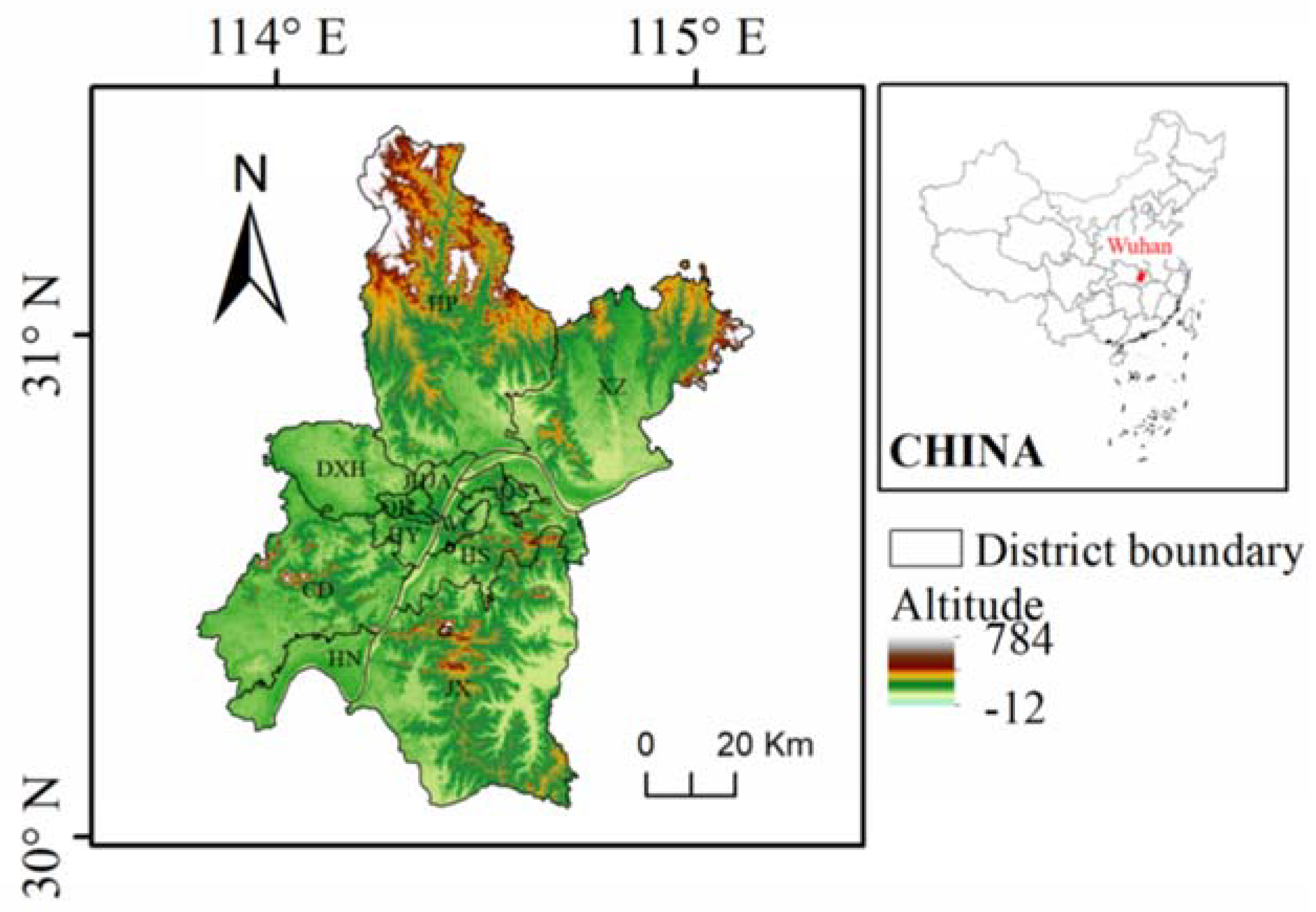
2.1.1. Study Area

Wuhan, the study area, is located in the east of the Hubei province, an important industrial, scientific, and educational base and comprehensive transportation hub in China. The terrain in the area is mainly made up of plains, which account for about 81.9% of the total area of the city (Figure 1). In 2020, the GDP reached CNY 1561.606 billion, and the urbanization rate was 80.49%, which was an increase of 0.2% over the previous year. The permanent population was about 9024.5 thousand with a birth rate of 12.8‰ and a mortality rate of 5.7‰. From 2010 to 2020, the annual growth rate of the Wuhan built-up area was 41.83%. While forest land and water bodies decreased by 0.65% and 0.79% from 2010 to 2015, with change rates of −52.71% and −55.29%, respectively (Figure 2). The Wuhan built-up area has continued to expand over the last 20 years. The Territorial Space Planning 2020–2035 (Draft) proposed to delineate the urban development boundary, lock the urban space, and give full play to Wuhan’s central role in the Hubei province and the urban circle.

2.1.2. Data Sources

The data used in this study include the following types: remote sensing data, nighttime satellite image, digital elevation model (DEM) data, land-use data, and socioeconomic statistical data. Land-use data and remote sensing data originate from the Geospatial Data Cloud (http://www.gscloud.cn/) (accessed on 20 January 2022).Considering the influence of cloud cover and season on remote sensing data, we selected landsat 5 TM images from 2010 and landsat 8 OLI images from 2015 and 2020 with orbit numbers 123/38 and 122/39 and a resolution of 30 m. Nighttime satellite images from 2010 were obtained from the National Oceanic and Atmospheric Administration (http://www.ngdc.noaa.gov) (accessed on 20 January 2022). DMSP/OLS nighttime light images were only available until 2013 with a resolution of 1 km, so in 2015 and 2020, we selected nighttime satellite images (NPP-VIIRS) with a resolution of 500 m. The grid data of population density and GDP distribution in 2015 came from the Data Center for Resource and Environmental Sciences, Chinese Academy of Sciences (http://www.resdc.cn/) (accessed on 20 January 2022), with a resolution of 1 km.

2.1.3. Data Processing

Interpretation of remote sensing data consisted of radiometric correction of the Landsat images and atmospheric correction using ENVI, and the remote sensing images of Wuhan were obtained by combining the vector boundary. Furthermore, through supervision and classification, land-use/land-cover (LULC) classes of Wuhan were divided into six categories: cultivated land, forest land, grass land, water bodies, built-up area, and unused land (Figure 2).

Nighttime light image processing was performed in ArcGIS, where the 2015 nighttime light data were resampled to a 1 km resolution to eliminate the impact of the different resolutions of the original images. We extracted the nighttime average light intensity data according to the boundary of the study area, reclassified them, and then extracted the area with the light value of the image pixel greater than 20 as the active area [28] (Figure 3). It can be seen that the range of active areas is expanding, and the high-value areas are increasing; however, it was difficult to obtain a complete closed area according to the night active areas of each year.

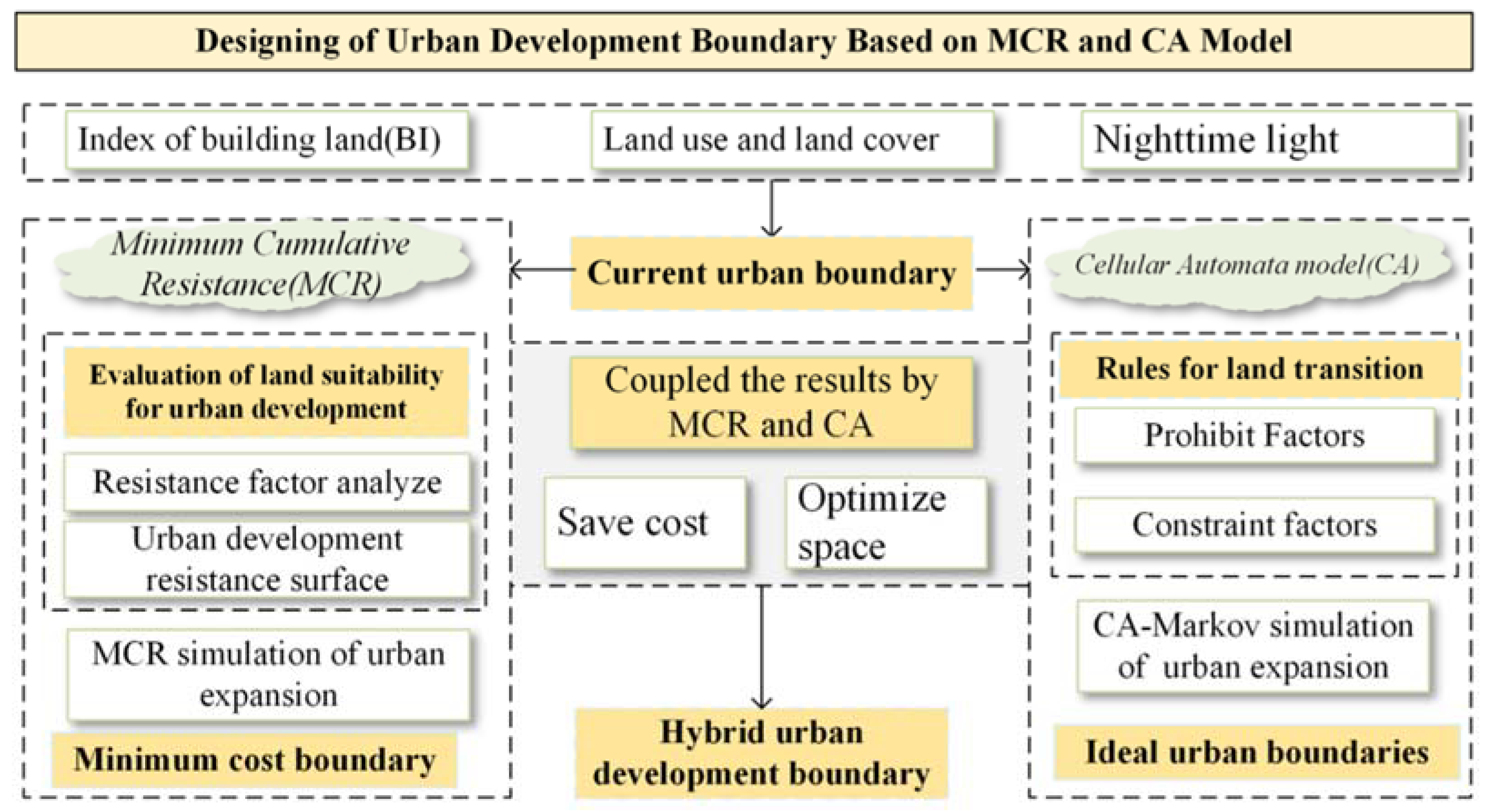
2.2. Research Framework

Through the interpretation of the new requirements of land and space planning in the new era, UDB should be defined according to the principles of rigid scale, micro-elastic layout, concentration, and regularity. In this study, we constructed a research framework from urban current boundary identification to UDB delineation (Figure 4).

On the basis of clarifying the connotation of UDB, the current urban boundary was extracted by combing the built-up index and nighttime light index, and the UDB was delineated by integrating the MCR model and CA-Markov model. Among them, the process of defining UBD by the MCR model was based on the analysis of the evolution characteristics of built-up areas in Wuhan and the threshold of the maximum effective supply scale of built-up areas that can be reached at present based on the regional real endowment conditions. This process focuses on the perspective of actual supply, and the boundary is delineated according to the idea of “determining the expansion source–analyzing the expansion resistance factor–constructing the expansion resistance surface–determining the suitability level of expansion”. The process of delineating UDB using the CA-Markov model is as follows: spatial location of the regional built-up area is simulated and predicted by grasping the regional land-use conversion rules and giving priority to meeting the demand of urban spatial expansion. This process focuses on the perspective of ideal land demand, defining the UDB according to the idea of “rule formulation—simulation comparison—accuracy test—result prediction”.

The delineation of UDB should not only ensure the rigid demand of urban development for land, but also meet the goal of sustainable development. Therefore, on the basis of the simulation results of the MCR and CA-Markov models, in this study, we extracted the overlapping parts and delineated the UDB, so as to achieve the goal of balancing urban land supply and demand.

2.3. Method

2.3.1. Extracting Current Built-Up Area

We eliminated the redundant built-up area outside the urban nighttime light active area and took the outsourcing network of the built-up area in the active area as the current urban boundary. Among them, the built-up area information was extracted using the built-up index (BI) [29,30], and the BI was generated as follows:

BI = NDBI × NDVI − MNDWI

(1)

where NDBI is the normalized building index, and the value is between [−1,1]. NDBI > 0 is a built-up area, and NDBI ≤ 0 is a non-built-up area. However, as a result of external factors such as season and sunlight, the calculation of NDBI was influenced by plants that simultaneously have the spectral characteristics of plants and a built-up area. Therefore, we were not able to extract urban built-up area well using only NDBI, and the impact of vegetation and water body needed to be eliminated. NDVI is the normalized vegetation index, and MNDWI is an improved normalized difference water body index.

2.3.2. Minimum Cumulative Resistance Model

The minimum cumulative resistance (MCR) model describes the resistance that species need to overcome in the process of moving from source to destination, which is implemented in the cost distance in ArcGIS. The MCR model was proposed by Knaapen in 1992 [31]. After the introduction of the MCR model by Yu et al. (2012), it has been widely used in the fields of species protection, landscape pattern analysis, and other areas [32,33,34]. Recently, Chinese scholars have begun to use the MCR model in socioeconomic fields such as tourism destination planning and land use [35,36]. On this basis, we integrated the MCR model into the study of urban spatial growth to simulate the trend of urban expansion. In this study, urban built-up area expansion is viewed as competition for a built-up area over other land-use types, and this competition must be achieved by overcoming resistance. In this way, urban built-up area expansion can be modeled as the process of overcoming resistance to expansion from urban building land sources. As a result of the spatial heterogeneity of land, cities are affected by resistance of different sizes in the expansion process. The MCR model is calculated as follows:

$$\mathrm{MCR}={\mathrm{f}}_{\min {\displaystyle \sum }_{\mathrm{j}=\mathrm{n}}^{\mathrm{i}=\mathrm{m}}{\mathrm{H}}_{\mathrm{ij}}\times {\mathrm{R}}_{\mathrm{i}}},$$

(2)

where MCR is the minimum cumulative resistance value of urban built-up area spreading, and H_ij is the distance from built-up area source j to space unit i at any point in space; Ri is the resistance coefficient of the spatial element i to the motion of any point in space; Σ is the accumulation of the distance and resistance across all the units between the space unit i and source j; min is the minimum cumulative resistance of the evaluated area to different sources; and f indicates that the minimum cumulative resistance is a positive correlation function with the ecological process.

The whole processing process was carried out in ArcGIS. The steps are as follows: (1) Determining the expansion source: “source” is the starting point of outward diffusion of things. On the basis of its nature and the nature of surrounding communication media, this shows different abilities to expand. We took the built-up area in the LUCC in 2020 as the expansion source. (2) Construction of resistance surface of urban expansion: urban spatial expansion needs to consider the suitability of surrounding land, and the degree of suitability is expressed by the resistance value. The resistance factors affecting urban expansion are selected, and the resistance surface is constructed by dividing grades and giving scores and weights. (3) Suitability analysis of urban expansion: the cost–distance function in ArcGIS is used to combine the expansion source with the resistance surface to obtain the minimum cumulative cost of each grid unit to the nearest “source” with the lowest cost. The cumulative cost can be regarded as the suitability of the “source” to expand. The natural breakpoint method is used to divide the suitability level of urban expansion.

2.3.3. CA-Markov Model

The CA-Markov model combines the functions of the CA model and Markov model [37]. It not only simulates the spatial change of complex systems, but also predicts the long-time series. Therefore, it is widely used to simulate the spatio-temporal change of land use [38]. The CA-Markov model uses a transfer matrix and suitability atlas to determine land-type changes and simulate LULC in a subsequent year. The processing runs in IDRISI and ArcGIS software, and the steps are as follows: (1) Using the Markov model, the land-use classes in 2015 are taken as the starting state, superimposing the land-use classes in 2020 to obtain the land-use transfer matrix from 2015 to 2020, so as to provide conversion rules for the land-use simulation. (2) On the basis of the analysis of the limiting and constraint factors of land-class conversion, the MCE module is used to make the suitability image of local class conversion, and the weighted linear combination method is selected to provide conversion rules for subsequent simulation operations. (3) The cellular automata filter is determined, the starting time is set as 2020 and the cycle times as 5 years, and prediction simulation is carried out.

3. Results

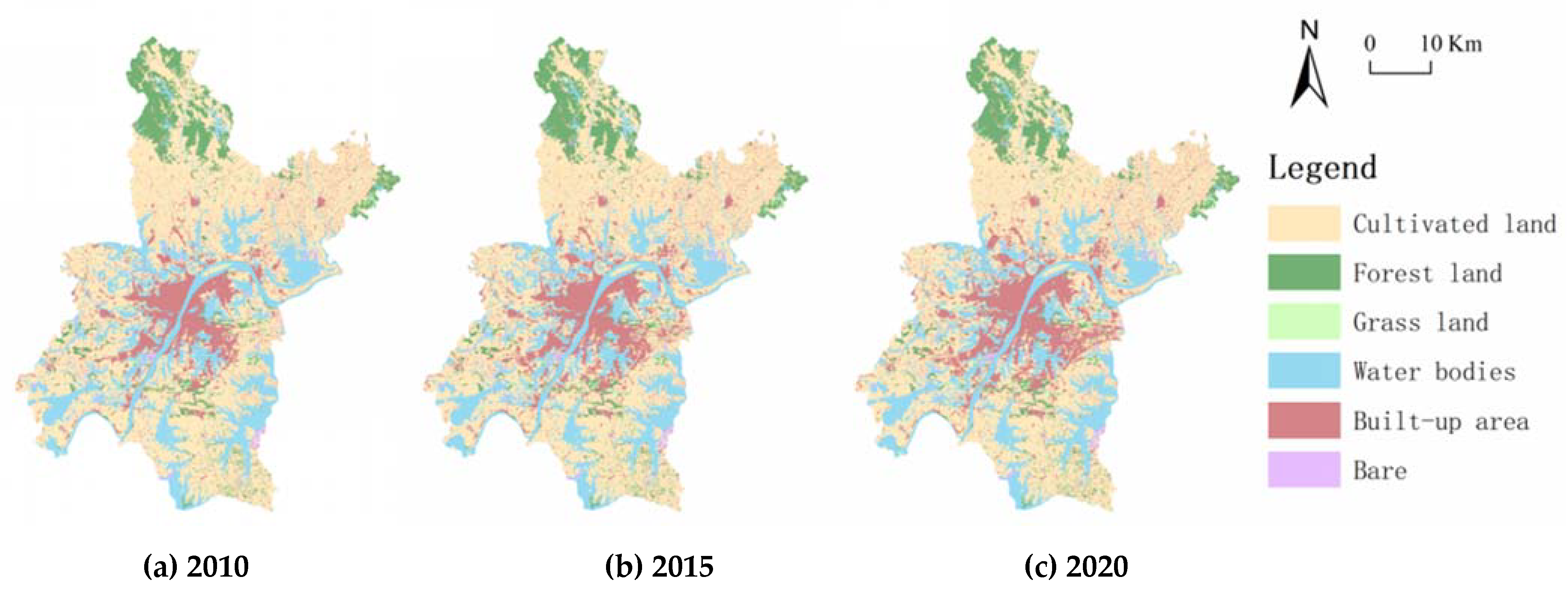
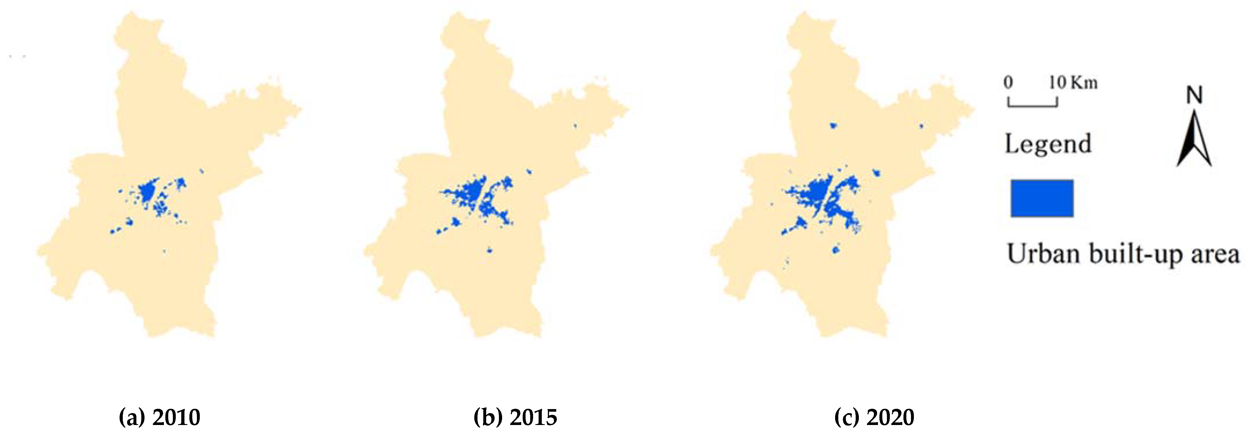
3.1. Identifying Built-Up Area in 2010, 2015, and 2020

Bandmath was used to calculate the NDBI, NDVI, MNDWI, and BI of phase III images in ENVI, and the area with BI > 0 was extracted in ArcGIS as the built-up area (Figure 5). The area with BI > 0 covers the built-up area of the urban center, but there are some built-up areas in villages and towns. It was difficult to extract a complete and closed boundary on this basis. This section provides a concise and precise description of the experimental results, their interpretation, and the experimental conclusions that can be drawn.

We extracted and overlaid the active area of nighttime light and the built-up area from the land-use data to obtain the urban built-up areas in 2010, 2015, and 2020 (Figure 6). According to the statistics, the built-up areas were 503 km², 568.13 km², and 887.56 km², respectively. The expansion direction of the urban built-up area was mainly in the south and northeast. This result is basically consistent with the built-up area and urban expansion direction of the urban development area in the Wuhan Urban Master Planning (2010–2020) [39].

3.2. Designing the Urban Development Boundary by MCR Model

3.2.1. Analysis of Resistance Factors of Urban Sprawl

This study selected eight resistance factors that affect urban expansion from three aspects: natural conditions, traffic and socioeconomic conditions, including land-use status, elevation, slope, distance from main roads, distance from branch road, distance from water bodies, population density, and GDP. Flat areas with low elevation, convenient transportation, a high population density, and a developed economy face less urban expansion resistance, and are thus more suitable for urban expansion and development. Contrarily, the greater the urban expansion resistance, the less suitable the area is for urban expansion and development. Referring to Liu et al.’s (2017) research in combination with the regulations for gradation and classification on urban land [40], we classified the resistance factors and weights, as shown in

Table 1. Resistance factor classification, scores, and weights.

Factors	Classification	Scores	Weights	Factors	Classification	Scores	Weights
The land–use status	Built–up land	5	0.15	Distance from the main road	0–1000	5	0.13
	Cultivated land	4			1000–2000	4
	Others	3			2000–3000	3
	Forestland and grassland	2			3000–4000	2
	Water bodies	1			>4000	1
Elevation	0–60	5	0.10	Distance from the branch road	0–500	5	0.10
	60–120	4			500–1000	4
	120–180	3			1000–1500	3
	180–240	2			1500–2000	2
	>240	1			>2000	1
Slope	0–2	5	0.14	GDP	<3000	5	0.13
	2–6	4			3000–8000	4
	6–15	3			8000–15000	3
	15–25	2			15000–30000	2
	>25	1			>30000	1
Distance from the water bodies	0–1000	5	0.12	The population density	<800	5	0.13
	1000–2000	4			800–2800	4
	2000–3000	3			2800–5000	3
	3000–4000	2			5000–8400	2
	>4000	1			>8400	1

[27].

3.2.2. Evaluation of Land Suitability of Urban Development

We derived each resistance factor value and calculated the comprehensive resistance surface using the distance analysis, reclassification, and raster calculation in the ArcGIS 10.7 software according to Table 1. We also derived the cumulative cost of urban expansion using the cost distance function in the ArcGIS 10.7 software. We then classified the cumulative cost of urban expansion by the natural breakpoint method to five suitability types: very high suitable, high suitable, medium suitable, low suitable, and very low suitable. The higher the suitability, the more conducive to urban expansion (Figure 7). The areas at a very high level and high level for urban development are mainly distributed around the developed urban built-up area and cultivated land near to the urban area, accounting for 58.78% and 9.18% of the total area, respectively. The areas at a low level for urban development are mainly cultivated land and forest land, which are distributed around the highly suitable areas in a strip or point shape, accounting for 7.07% of the total area. The areas at a low and very low level are mainly forest land and water bodies on the edge of the city, mainly located in the northwest of Wuhan, accounting for 8.71% and 16.26% of the total area, respectively.

3.2.3. Urban Development Boundary Results Using the MCR Model

On the basis of the results of the MCR model, we selected areas with very high and high suitabilities of urban expansion as the urban expansion area in the predicted years, and removed the scattered and fragmented patches and kept the aggregated patches. In this way, the UDBs in 2025, 2030, and 2035 were delineated, with total areas of 903.52 km², 937.48 km², and 1021.44 km², respectively. The areas of built-up area within the UDB derived from the MCR method were 672.31 km², 695.45 km², and 712.83 km² in 2025, 2030, and 2035, respectively (Figure 8). It was found that the urban space of Wuhan will sprawl southward.

3.3. Designing the Urban Development Boundary Using the CA-Markov Model

3.3.1. Rules for Land-Cover Transition in the CA-Markov Model

As the limiting factor of land-type conversion, the built-up area, cultivated land, and water bodies can be converted in areas with a slope of less than 6°, and forest land, grass land, and unused land can be converted in areas with a slope of more than 6°. Water bodies cannot be used for built-up area conversion, so it was set as the limiting factor of construction conversion [25]. It is hard to convert a built-up area into cultivated land, so a built-up area was regarded as the limiting factor of cultivated land. The constraint factor was standardized using the fuzzy function, and the value range was 0~255.

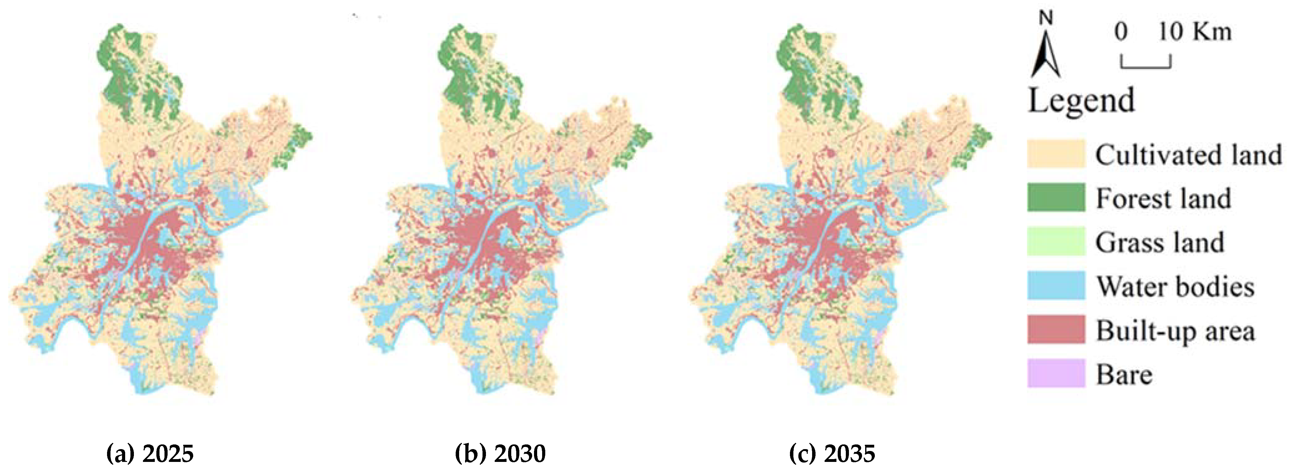
3.3.2. Simulation Results and Accuracy

On the basis of the land-use transfer matrix and suitability atlas, we used the CA-Markov model to simulate the land-use situation in 2020 and compare it with the actual land use in 2020 (

Table 2. Analysis of land-use simulation errors of Wuhan City in 2020.

Land Use	Simulated Area (km2)	Actual Area (km2)	Quantity Error (%)	Spatial Error (%)
Cultivated land	4529.01	4781.98	−5.29	2.41
Built-up land	1267.44	1140.19	11.16	6.33
Forestland and grassland	883.05	850.91	3.78	8.60
Water bodies	1822.36	1730.86	5.29	7.04
Unused land	73.19	71.11	2.93	7.58

). The simulation results produce a Kappa index of 0.91 (>0.75), indicating that they are accurate [41,42]. The errors of forestland, grassland, and unused land were all below 5%. Although the error of the built-up area was relatively high, it was still within an acceptable range. Therefore, we used this model to simulate and predict land use in 2025, 2030, and 2035 (Figure 9).

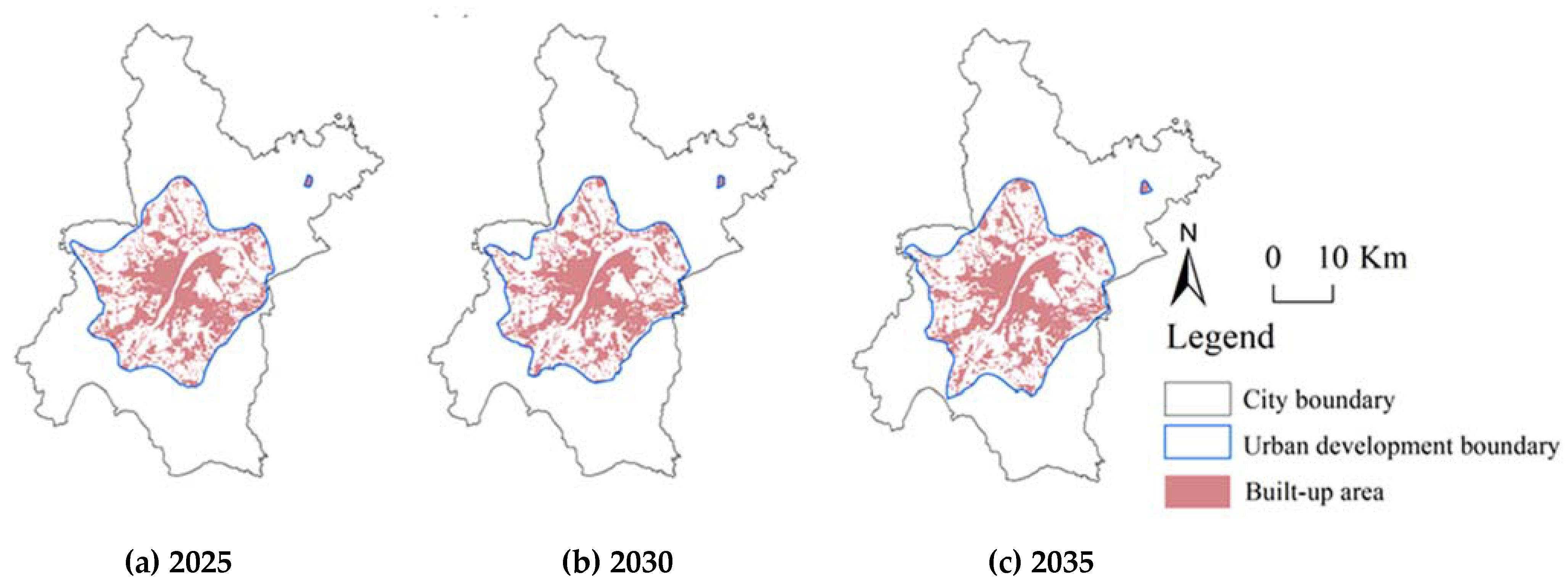
3.3.3. Urban Development Boundary Results Using the CA-Markov Model

We extracted the built-up area from the simulation results of 2025, 2030, and 2035 in the ArcGIS 10.7 software, then removed the scattered and broken patches and kept the aggregated patches. The areas of built-up area in each year were 689.71 km², 702.54 km², and 747.29 km², respectively. We delineated the UDB of Wuhan City according to the outsourcing surface of built-up land in 2025, 2030, and 2035 (Figure 10). The areas of each boundary were 912.75 km², 946.40 km², and 1041.91 km², respectively. The expansion trend of the built-up area demonstrates that the urban area of Wuhan will continually expand.

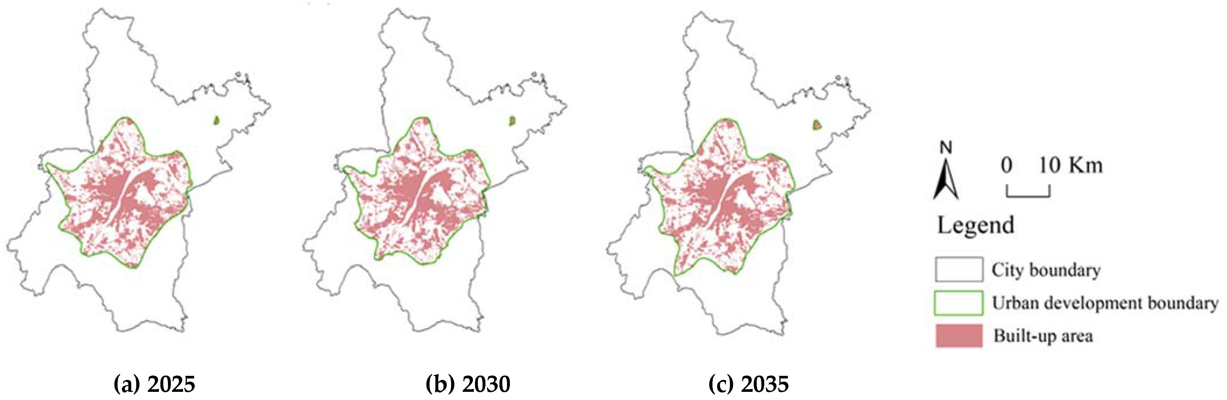
3.4. Combing the Results of the MCR Model and CA-Markov Model

Using both the MCR and CA-Markov models, we were able to delineate the UBD of Wuhan City from different perspectives; however, the delineation results were marginally different. On the basis of the MCR model, the UBD scales from the perspective of the minimum cost of Wuhan City in 2025, 2030, and 2035 were 903.52 km², 937.48 km², and 1021.44 km², respectively. On the basis of the CA-Markov model, the UBD areas of Wuhan City from the perspective of ideal land demand in 2025, 2030, and 2035 were 912.75 km², 946.40 km², and 1041.912 km², respectively. The UBDs delineated by the MCR model were smaller than the UBDs delineated by the CA-Markov model. Spatially, the change trends of UBD from the two methods were consistent, mainly expanding to the south of Wuhan, although there were some minor differences. Therefore, it was necessary to devise a rational UBD for regional territorial space planning to achieve supply–demand balance.

The MCR model considers the suitability level of urban expansion of the regional landscape from the perspective of actual land supply to delineate the UBD. The CA model predicts future changes based on the land-type conversion rules, thus delineating the UBD from the perspective of ideal land demand. If the UBD was only delineated by the MCR model, although it follows the suitability level and reaches the minimum cost of land supply, it does not consider the demand of urban development for land. If the UBD was only delineated by the CA model, although it follows the rules of land-use and land-cover changes, it seldom considers the urban expansion cost, so it is hard to achieve the requirements of sustainable development. In view of this, we overlapped the results based on the MCR model and CA model and selected a shared area as the UBD to realize the balance of supply and demand of urban development. The final UBDs of Wuhan City in 2025, 2030, and 2035 were 901.62 km², 944.39 km², and 1015.36 km², respectively (Figure 11).

4. Discussion

4.1. Comparison with Existing Research

With rapid industrialization and urbanization, the extensive and inefficient use of land under rapid socioeconomic development is ignored. How to improve land-use efficiency during rapid urbanization has become an urgent problem in social development [43,44]. For this reason, China has established a series of land management laws and relevant regulations to promote the intensive use of urban construction land. Among them, the regulations on economical and intensive land [45] issued by the Ministry of Land and Resources of the People’s Republic of China in 2014 describes the definition, connotation, and methods of economical and intensive land benefits. The delineation of the city development boundary as a rigid boundary to restrict the expansion of city land can also effectively stimulate the intensive development of city land [46]. The urbanization rate of Wuhan City was 77.07% in 2010, 79.41% in 2015, and 84.3% in 2020, and the annual average growth rate was 1.29%. The urban space expanded at the rate of 38.45m² per year from 2010 to 2020, indicating that the urbanization of Wuhan is rapid. The average annual growth of urban space in Wuhan from 2020 to 2030 simulated in this study is 11.37 km², which is in line with the spatial evolution pattern of Wuhan. The growth rate of the boundary is reduced compared with the previous rate, which is conducive to promoting the economical and intensive development of the city and meeting the requirements of urban sustainable development in the future [47,48].

The 2020 UBD delineated in this study is consistent with the pattern of boundary expansion in the Wuhan Urban Master Planning (2010-2020) [39]. Hankou, Hanyang, and Wuchang, located in the urban center, are the core of future urban development. Most areas of Hanyang and Hongshan, and some areas of Dongxihu, Caidian, Jiangxia, and Huangpi, have also become centers of urban development and expansion. Wuhan’s urban space shows a trend of radiating and expanding from the central urban area to the surrounding areas (Figure 10), especially in the south and northeast of Wuhan, which is closely related to Wuhan’s policies to accelerate the construction of the Yangtze River Economic Belt and is in line with the urban space development trend of “one master and four deputies”. Moreover, He et al. (2017) and Zhai et al. (2021) found that when simulating the urban spatial expansion of Wuhan, it mainly concentrated in the edges of the Hanyang and Hongshan Districts [49,50], which is consistent with the findings of this study. In addition, the UDB of Wuhan is lower than the expansion scale of the built-up area predicted by Liang et al. (2021) and Wang et al. (2021) [51,52]. This indicates that the urban development boundary defined in this study is more restrictive than other studies in constraining the expansion of urban land; therefore, the method proposed herein is scientific and superior to other scholars’ methods to a certain extent.

4.2. Strength and Limitations

How to achieve the rational, orderly, and sustainable development of cities has always been a hot topic in China’s urbanization research. Moreover, the rational delineation of the urban development boundary as an effective means to control the disorderly expansion and restrict the healthy development of cities has attracted attention from scholars [49,50]. In this context, a series of mathematical models for the urban development boundary have emerged [12,51,52]. Many scholars build ANN models and CA models combining GIS and remote-sensing technology to simulate and predict the urban growth boundary, but these only delineate the urban development boundary according to the regularity of spatial evolution of land use and land cover. This study integrates the urban expansion trend (CA) and the urban expansion cost (MCR) and constructs a coupled model to delineate the future urban development boundary with Wuhan as the research area. This method not only ensures the rigid demand for land for urban development and the cost of urban expansion, but also meets the requirements of economic intensive land use and regional space planning. Furthermore, it is widely applicable to China’s growing cities, such as Changsha, Zhengzhou, and other big cities. In other cities, the method proposed in this study still has certain reference significance. However, as a result of differences in the natural environment, population density, land policy, development goals, etc., we need to consider the regional characteristics of the study area and other restrictive factors when using it, and then adjust the parameter settings of the model. For example, the control policies of European and American countries are basically bottom-up, and the control policies are mostly formulated by the municipal and state governments. The main purpose of UDB is to solve the problem of inefficient land use caused by counter-urbanization and suburbanization and protect the ecological environment around the city. Conversely, China’s control policies are mostly top-down, with the country, province, city, county, and township being conducted downward at every level. In addition, the main purpose of delineating UDB is to optimize urban layout and sustainable development. There are obvious differences between the two. Therefore, regional adjustments need to be made in consideration of limiting factors and model parameters when using the method in other cities.

There are certain deficiencies to be further explored in this study. First, the theoretical analysis of the impact mechanism of the delineation of the boundary between prohibited development zones and urban development such as basic farmland and ecological land is not sufficient [53]. Second, the data processing methods and accuracy of traditional remote-sensing data, nighttime light data, and routine survey changes data need to be improved. Third, this study does not simulate LULC in a multi-scenario [51]. In the future, scholars should simulate LULC prediction based on a multi-scenario, so as to make the evaluation results have greater reference value.

5. Conclusions

To provide a scientific reference for urban development planning, we delineated the urban development boundary based on the MCR model and CA models. The research results are as follows:

(1) Identifying the built-up area shows that the built-up areas of Wuhan in 2010, 2015, and 2020 were 503 km², 568.13 km², and 887.56 km², respectively, and the urban spatial expansion direction was mainly in the south and northeast, which is consistent with the urban planning strategy and actual construction situation of Wuhan;

(2) The MCR model’s empirical results show that by determining the suitability level of urban expansion, the MCR model constructed in this study defined the development boundary scale of Wuhan in 2025, 2030, and 2035 as 903.52 km², 937.48 km², and 1021.44 km², respectively, with an average annual growth of 11.79 km², representing the background conditions for urban supply expansion;

(3) The CA-Markov model’s empirical results show that the CA model constructed in this study has a high simulation accuracy, with a kappa coefficient of 0.91. Combined with the simulated land-use types, the development boundary scales of Wuhan in 2025, 2030, and 2035 will be 912.75 km², 946.40 km², and 1041.912 km², respectively, with an average annual growth of 12.91 km², which meets the requirements of orderly urban development;

(4) Comprehensive trade-off: the MCR and CA models were used to delineate the urban development boundary of Wuhan from the perspective of real supply and ideal land demand, respectively; however, the delineation results of the two methods were marginally different, and the delineation results based on the MCR model were less than those of the CA model. This study integrates the delineation results of the MCR and CA models in a comprehensive trade-off to recommend spatial ranges of 901.62 km², 944.39 km², and 1015.36 km², which serve as the urban development boundary of Wuhan in 2025, 2030, and 2035, respectively.

References

1. Liu, F.; Zhang, Z.; Shi, L.; Zhao, X.; Xu, J.; Yi, L.; Liu, B.; Wen, Q.; Hu, S.; Wang, X.; et al. Urban Expansion in China and Its Spatial-Temporal Differences over the Past Four Decades. J. Geogr. Sci. 2016, 26, 1477–1496. [Google Scholar] [CrossRef]
2. Zhao, S.; Zhou, D.; Zhu, C.; Qu, W.; Zhao, J.; Sun, Y.; Huang, D.; Wu, W.; Liu, S. Rates and Patterns of Urban Expansion in China’s 32 Major Cities over the Past Three Decades. Landsc. Ecol. 2015, 30, 1541–1559. [Google Scholar] [CrossRef]
3. Zhao, M.; Cai, H.; Qiao, Z.; Xu, X. Influence of Urban Expansion on the Urban Heat Island Effect in Shanghai. Int. J. Geogr. Inf. Sci. 2016, 30, 2421–2441. [Google Scholar] [CrossRef]
4. Jiang, X.; Lu, X. Temporal and Spatial Characteristics of Coupling and Coordination Degree Between Urbanization and Human Settlement of Urban Agglomerations in the Middle Reaches of the Yangtze River. China Land Sci. 2020, 34, 25–33. [Google Scholar]
5. Wang, J.; Fang, C. Growth of Urban Construction Land: Progress and Prospect. Prog. Geogr. 2011, 30, 1440–1448. [Google Scholar]
6. Chen, Y.; Zhang, Z.; Du, S.; Shi, P.; Tao, F.; Doyle, M. Water Quality Changes in the World’s First Special Economic Zone, Shenzhen, China. Water Resour. Res. 2011, 47, W11515. [Google Scholar] [CrossRef]
7. Shi, K.; Shen, J.; Wang, L.; Ma, M.; Cui, Y. A Multiscale Analysis of the Effect of Urban Expansion on PM2.5 Concentrations in China: Evidence from Multisource Remote Sensing and Statistical Data. Build. Environ. 2020, 174, 106778. [Google Scholar] [CrossRef]
8. Colsaet, A.; Laurans, Y.; Levrel, H. What Drives Land Take and Urban Land Expansion? A Systematic Review. Land Use Policy 2018, 79, 339–349. [Google Scholar] [CrossRef]
9. Larsen, K. New Urbanism’s Role in Inner-City Neighborhood Revitalization. Hous. Stud. 2005, 20, 795–813. [Google Scholar] [CrossRef]
10. Siedentop, S.; Fina, S.; Krehl, A. Greenbelts in Germany’s Regional Plans—An Effective Growth Management Policy? Landsc. Urban Plan. 2016, 145, 71–82. [Google Scholar] [CrossRef]
11. Naldi, L.; Nilsson, P.; Westlund, H.; Wixe, S. What Is Smart Rural Development? J. Rural Stud. 2015, 40, 90–101. [Google Scholar] [CrossRef]
12. Tayyebi, A.; Pijanowski, B.C.; Tayyebi, A.H. An Urban Growth Boundary Model Using Neural Networks, GIS and Radial Parameterization: An Application to Tehran, Iran. Landsc. Urban Plan. 2011, 100, 35–44. [Google Scholar] [CrossRef]
13. Kline, J.D.; Alig, R.J. Does Land Use Planning Slow the Conversion of Forest and Farm Lands? Growth Change 1999, 30, 3–22. [Google Scholar] [CrossRef]
14. Lu, Y.; Li, X.; Ni, H.; Chen, X.; Xia, C.; Jiang, D.; Fan, H. Temporal-Spatial Evolution of the Urban Ecological Footprint Based on Net Primary Productivity: A Case Study of Xuzhou Central Area, China. Sustainability 2019, 11, 199. [Google Scholar] [CrossRef] [Green Version]
15. Jiang, P.; Cheng, Q.; Gong, Y.; Wang, L.; Zhang, Y.; Cheng, L.; Li, M.; Lu, J.; Duan, Y.; Huang, Q.; et al. Using Urban Development Boundaries to Constrain Uncontrolled Urban Sprawl in China. Ann. Am. Assoc. Geogr. 2016, 106, 1321–1343. [Google Scholar] [CrossRef]
16. Zhang, J.; Yuan, X.; Tan, X.; Zhang, X. Delineation of the Urban-Rural Boundary through Data Fusion: Applications to Improve Urban and Rural Environments and Promote Intensive and Healthy Urban Development. Int. J. Environ. Res. Public Health 2021, 18, 7180. [Google Scholar] [CrossRef]
17. Zheng, B.; Liu, G.; Wang, H.; Cheng, Y.; Lu, Z.; Liu, H.; Zhu, X.; Wang, M.; Yi, L. Study on the Delimitation of the Urban Development Boundary in a Special Economic Zone: A Case Study of the Central Urban Area of Doumen in Zhuhai, China. Sustainability 2018, 10, 756. [Google Scholar] [CrossRef] [Green Version]
18. Harig, O.; Hecht, R.; Burghardt, D.; Meinel, G. Automatic Delineation of Urban Growth Boundaries Based on Topographic Data Using Germany as a Case Study. ISPRS Int. J. Geo-Inf. 2021, 10, 353. [Google Scholar] [CrossRef]
19. Tayyebi, A.; Perry, P.C.; Tayyebi, A.H. Predicting the Expansion of an Urban Boundary Using Spatial Logistic Regression and Hybrid Raster-Vector Routines with Remote Sensing and GIS. Int. J. Geogr. Inf. Sci. 2014, 28, 639–659. [Google Scholar] [CrossRef]
20. Zhang, J. Urban Growth Management in the United States. Urban Plan. Overseas 2002, 2, 37–40. [Google Scholar]
21. Zhuang, Z.; Li, K.; Liu, J.; Cheng, Q.; Gao, Y.; Shan, J.; Cai, L.; Huang, Q.; Chen, Y.; Chen, D. China’s New Urban Space Regulation Policies: A Study of Urban Development Boundary Delineations. Sustainability 2017, 9, 45. [Google Scholar] [CrossRef] [Green Version]
22. Liang, X.; Liu, X.; Li, X.; Chen, Y.; Tian, H.; Yao, Y. Delineating Multi-Scenario Urban Growth Boundaries with a CA-Based FLUS Model and Morphological Method. Landsc. Urban Plan. 2018, 177, 47–63. [Google Scholar] [CrossRef]
23. Zhenbo, W.; Qiang, Z.; Xiaorui, Z. Urban Growth Boundary Delimitation of Hefei City Based on the Resources and Environment Carrying Capability. Geogr. Res. 2013, 32, 2301–2311. [Google Scholar]
24. Torrens, P.M. Simulating Sprawl. Ann. Assoc. Am. Geogr. 2006, 96, 248–275. [Google Scholar] [CrossRef]
25. Han, J.; Hayashi, Y.; Cao, X.; Imura, H. Application of an Integrated System Dynamics and Cellular Automata Model for Urban Growth Assessment: A Case Study of Shanghai, China. Landsc. Urban Plan. 2009, 91, 133–141. [Google Scholar] [CrossRef]
26. Zhou, R.; Wang, X.; Hailong, S.U.; Qian, X.; Sun, B. Delimitation of Urban Growth Boundary Based on Ecological Security Pattern. Urban Plan. Forum 2014, 4, 57–63. [Google Scholar]
27. Liu, G.; Liang, Y.; Cheng, Y.; Wang, H.; Yi, L. Security Patterns and Resistance Surface Model in Urban Development: Case Study of Sanshui, China. J. Urban Plan. Dev. 2017, 143, 05017011. [Google Scholar] [CrossRef]
28. Liu, Q.; Yang, Y.; Fu, D.; Li, H.; Tian, H. Urban Spatial Expansion Based on DMSP_OLS Nighttime Light Data in China in 1992–2010. J. Geogr. Sci. 2014, 34, 129–136. [Google Scholar]
29. He, C.; Shi, P.; Xie, D.; Zhao, Y. Improving the Normalized Difference Built-up Index to Map Urban Built-up Areas Using a Semiautomatic Segmentation Approach. Remote Sens. Lett. 2010, 1, 213–221. [Google Scholar] [CrossRef] [Green Version]
30. Varshney, A.; Rajesh, E. A Comparative Study of Built-up Index Approaches for Automated Extraction of Built-up Regions From Remote Sensing Data. J. Indian Soc. Remote Sens. 2014, 42, 659–663. [Google Scholar] [CrossRef]
31. Knaapen, J.P.; Scheffer, M.; Harms, B. Estimating Habitat Isolation in Landscape Planning. Landsc. Urban Plan. 1992, 23, 1–16. [Google Scholar] [CrossRef]
32. Dai, L.; Liu, Y.; Luo, X. Integrating the MCR and DOI Models to Construct an Ecological Security Network for the Urban Agglomeration around Poyang Lake, China. Sci. Total Environ. 2021, 754, 141868. [Google Scholar] [CrossRef]
33. Li, H.; Peng, J.; Yanxu, L.; Yi’na, H. Urbanization Impact on Landscape Patterns in Beijing City, China: A Spatial Heterogeneity Perspective. Ecol. Indic. 2017, 82, 50–60. [Google Scholar] [CrossRef]
34. Ye, H.; Yang, Z.; Xu, X. Ecological Corridors Analysis Based on MSPA and MCR Model-A Case Study of the Tomur World Natural Heritage Region. Sustainability 2020, 12, 959. [Google Scholar] [CrossRef] [Green Version]
35. Chen, Y.; Li, X.; Liu, X.; Huang, H.; Ma, S. Simulating Urban Growth Boundaries Using a Patch-Based Cellular Automaton with Economic and Ecological Constraints. Int. J. Geogr. Inf. Sci. 2019, 33, 55–80. [Google Scholar] [CrossRef]
36. Li, P.; Cao, H. Simulating Uneven Urban Spatial Expansion under Various Land Protection Strategies: Case Study on Southern Jiangsu Urban Agglomeration. ISPRS Int. Geo-Inf. 2019, 8, 521. [Google Scholar] [CrossRef] [Green Version]
37. Kamusoko, C.; Aniya, M.; Adi, B.; Manjoro, M. Rural Sustainability under Threat in Zimbabwe-Simulation of Future Land Use/Cover Changes in the Bindura District Based on the Markov-Cellular Automata Model. Appl. Geogr. 2009, 29, 435–447. [Google Scholar] [CrossRef]
38. Guan, D.; Gao, W.; Watari, K.; Fukahori, H. Land Use Change of Kitakyushu Based on Landscape Ecology and Markov Model. J. Geogr. Sci. 2008, 18, 455–468. [Google Scholar] [CrossRef]
39. Hubei Provincial People’s Government. Wuhan Urban Master Planning (2010–2020). 2010. Available online: http://gtghj.wuhan.gov.cn/dxh/pc-998-108001.html (accessed on 20 January 2022).
40. General Administration of Quality Supervision, Inspection and Quarantine of the People’s Republic of China, AQSIQ. Regulations for Gradation and Classification on Urban Land; AQSIQ: Beijing, China, 2014. Available online: http://c.gb688.cn/bzgk/gb/showGb?type=online&hcno=BD27E38FDD9A5B296739FD976FC0707C (accessed on 20 January 2022).
41. De Oliveira Barros, K.; Ribeiro, C.A.A.S.; Marcatti, G.E.; Lorenzon, A.S.; de Castro, N.L.M.; Domingues, G.F.; de Carvalho, J.R.; dos Santos, A.R. Markov Chains and Cellular Automata to Predict Environments Subject to Desertification. J. Environ. Manag. 2018, 225, 160–167. [Google Scholar] [CrossRef]
42. Yang, X.; Bai, Y.; Che, L.; Qiao, F.; Xie, L. Incorporating Ecological Constraints into Urban Growth Boundaries: A Case Study of Ecologically Fragile Areas in the Upper Yellow River. Ecol. Indic. 2021, 124, 107436. [Google Scholar] [CrossRef]
43. Bai, X.; Shi, P.; Liu, Y. Realizing China’s Urban Dream. Nature 2014, 509, 158–160. [Google Scholar] [CrossRef] [Green Version]
44. Yang, J.; Jin, G.; Huang, X.; Chen, K.; Meng, H. How to Measure Urban Land Use Intensity? A Perspective of Multi-Objective Decision in Wuhan Urban Agglomeration, China. Sustainability 2018, 10, 3874. [Google Scholar] [CrossRef] [Green Version]
45. The Ministry of Land and Resources of the People’s Republic of China. Regulations on Economical and Intensive Land; The Ministry of Land and Resources of the People’s Republic of China: Beijing, China, 2014. Available online: http://gi.mnr.gov.cn/201908/t20190813_2458555.html (accessed on 20 January 2022).
46. Peng, C.; Song, M.; Han, F. Urban Economic Structure, Technological Externalities, and Intensive Land Use in China. J. Clean. Prod. 2017, 152, 47–62. [Google Scholar] [CrossRef]
47. Fu, J.; Xiao, G.; Wu, C. Urban Green Transformation in Northeast China: A Comparative Study with Jiangsu, Zhejiang and Guangdong Provinces. J. Clean. Prod. 2020, 273, 122551. [Google Scholar] [CrossRef]
48. Pickett, S.T.A.; Boone, C.G.; McGrath, B.P.; Cadenasso, M.L.; Childers, D.L.; Ogden, L.A.; McHale, M.; Grove, J.M. Ecological Science and Transformation to the Sustainable City. Cities 2013, 32, S10–S20. [Google Scholar] [CrossRef]
49. He, Q.; Liu, Y.; Zeng, C.; Chaohui, Y.; Tan, R. Simultaneously Simulate Vertical and Horizontal Expansions of a Future Urban Landscape: A Case Study in Wuhan, Central China. Int. J. Geogr. Inf. Sci. 2017, 31, 1907–1928. [Google Scholar] [CrossRef]
50. Zhai, H.; Lv, C.; Liu, W.; Yang, C.; Fan, D.; Wang, Z.; Guan, Q. Understanding Spatio-Temporal Patterns of Land Use/Land Cover Change under Urbanization in Wuhan, China, 2000–2019. Remote Sens. 2021, 13, 3331. [Google Scholar] [CrossRef]
51. Liang, X.; Guan, Q.; Clarke, K.C.; Liu, S.; Wang, B.; Yao, Y. Understanding the Drivers of Sustainable Land Expansion Using a Patch-Generating Land Use Simulation (PLUS) Model: A Case Study in Wuhan, China. Comput. Environ. Urban Syst. 2021, 85, 101569. [Google Scholar] [CrossRef]
52. Wang, H.; Liu, Y.; Zhang, G.; Wang, Y.; Zhao, J. Multi-Scenario Simulation of Urban Growth under Integrated Urban Spatial Planning: A Case Study of Wuhan, China. Sustainability 2021, 13, 11279. [Google Scholar] [CrossRef]
53. Hersperger, A.M.; Grădinaru, S.; Oliveira, E.; Pagliarin, S.; Palka, G. Understanding Strategic Spatial Planning to Effectively Guide Development of Urban Regions. Cities 2019, 94, 96–105. [Google Scholar] [CrossRef]
Figure 1. Location and altitude (m) of Wuhan city.
Land 11 00401 g001
Figure 2. Land cover of Wuhan City in (a) 2010, (b) 2015, and (c) 2020.
Land 11 00401 g002
Figure 3. Nighttime light of Wuhan City in (a) 2010, (b) 2015, and (c) 2020.
Land 11 00401 g003
Figure 4. Research framework.
Land 11 00401 g004
Figure 5. Built-up area in Wuhan city in (a) 2010, (b) 2015, and (c) 2020.
Land 11 00401 g005
Figure 6. Urban built-up areas of Wuhan city in (a) 2010, (b) 2015, and (c) 2020.
Land 11 00401 g006
Figure 7. Suitability levels of urban expansion.
Land 11 00401 g007
Figure 8. Urban development boundary for (a) 2025, (b) 2030, and (c) 2035 simulated by the MCR model.
Land 11 00401 g008
Figure 9. Land-cover predictions for (a) 2025, (b) 2030, and (c) 2035 using the CA-Markov model.
Land 11 00401 g009
Figure 10. Urban development boundary for (a) 2025, (b) 2030, and (c) 2035 simulated by the CA-Markov model.
Land 11 00401 g010
Figure 11. Hybrid urban development boundary of Wuhan city in (a) 2025, (b) 2030, and (c) 2035.
Land 11 00401 g011