Simulations of Soil Water and Heat Processes for No Tillage and Conventional Tillage Systems in Mollisols of China

Abstract

Soil water and temperature are important factors to reflect variations in soil heat and water flows especially for tillage systems. The objective of this study was to evaluate the performance of the CoupModel in predicting the effect of tillage practices on soil water and heat processes for conventional tillage (CT) and no-tillage (NT) systems with straw mulching on semi-arid and high-latitude Mollisols of northeast China. This model was calibrated and evaluated in a three-year tillage experiment from 2009 to 2011 in a field experiment station, using field measurements of daily soil temperature and water storage in profiles for CT and NT separately. The results showed that under the model, soil temperatures were well simulated at 0–90 cm soil depths for CT, as indicated by R² ≥ 0.97, the nRMSE = 27.5–38.7% and −1.02 °C ≤ ME ≤ −0.31 °C, and soil water storage at 0–130 cm soil depth (R² = 0.01–0.06, the nRMSE = 19.6–37.1%, 13.3 mm ≤ ME ≤ 28.2 mm) was simulated with more uncertainty. “Moderate to good agreements” were achieved for NT. In general, the temporal and spatial variations of soil temperature and water for NT were well simulated by CoupModel. Although NT decreased soil evaporation—thus improving soil water content, especially in the root zone soil—and lowered the soil frozen depths, it reduced the soil temperatures, which could influence crop growth. It was concluded that the CoupModel proved to be a functional tool to predict soil heat and water processes for CT and NT systems in high-latitude seasonal frost conditions of Mollisols in China to estimate the soil temperature, water, energy balance, and frost depth dynamics in relatively complex systems that combined plant dynamics with tillage and/or no tillage covered with straw mulching in the soil surface.

1. Introduction

China’s Mollisols (Udolls) belt is one of the four Mollisols belts in the world, which is mainly distributed in northeast China, including Heilongjiang, Jilin, and Liaoning provinces and part of the Inner Mongolian Autonomous Region. It covers approximately 1,030,000 km² and nearly 70% of it is in Heilongjiang province [1,2]. Located at 46–53° N, this province has a cool and humid continental climate, subject to seasonal freezing and thawing [3]. Soil erosion, water scarcity, and lower temperature in spring are common factors affecting crop production in this area and other similar regions. In the spring season, strong winds, lower temperature, and drought are three main limitations on planting, germination, and emergence, as well as the early growth of crops [4,5]. In the summer season, high air temperature is suitable for crop growth but variable and irregular rainfall would disrupt crop growth and soil condition, especially the heavy rainfall in August which would intensify soil and nutrient erosion in some fields with a slope > 5% [6], badly affecting the harvested area and yield [4,7].

The arable Mollisols have been intensively tilled for decades, leading to serious soil structural degradation and soil erosion [8]. In consequence, crop yields declined in these regions. Conservation tillage, together with soil surface cover and rotation, have been considered as the best management practices, which can reduce soil surface runoff, decrease soil erosion and evaporation [6,9,10], improve soil water content in the spring season, increase aggregate stability and bulk density, and decrease soil temperature in the summer season [11,12]. Thus, regulating soil water and heat environments is important for the arable Mollisols region. Soil temperature and water are two key factors that reflect variations in soil heat and water flow. However, tillage experiments are usually expensive, tedious, time and labor consuming, and it takes a long time to understand the responses of soil water and heat environments to the change in tillage and rotations [13]. In contrast, model simulation is a feasible tool to provide insights into the best crop management and environmental conditions such as soil water, heat, and nutrient dynamics, and their interactions with different cropping systems [14].

During the past five decades, many soil simulation models have been developed to achieve these objectives as reviewed by Whisler et al. [15], Bouman et al. [16], and Brisson et al. [17]. Some models focus on soil heat and water processes without plants, i.e., Hudrus [18] and SHAW [19,20]. Some soil heat and water models included a simple interface of plant or residue as a layer, i.e., SiSPAT [21], PILOTE [13,22], and CoupModel [23,24]. The CoupModel is one of the SVAT models. This physically based one-dimensional model consists of different coupled sub-models, soil dynamics (i.e., it integrates a predeveloped soil organic carbon and nitrogen model), and soil heat and water processes (i.e., it accounts for each component of soil heat and water flows in soil–plant–atmosphere systems). For model calibrations, the generalized likelihood uncertainty estimation (GLUE) method [25], as a common uncertainty analysis method, is used in CoupModel to assess the uncertainty of parameters, input data, and model structures and estimate the model output errors [3,26,27].

The objectives of this study were to: (1) calibrate a simulation model for describing the variation of soil temperature and soil water storage at different soil depths of conventional tillage systems over three years, and determine soil and vegetation input conditions that agree with the reality as closely as possible and assess the quality of the simulation results with the measured data of no-tillage systems with soil temperature and water data; (2) apply the CoupModel to predict soil heat and water processes, i.e., soil energy balance and soil evaporation, surface soil water as well as the frozen depth dynamics on clay loam soil in humid cool climate conditions with relatively complex systems of combining soil tillage and no tillage, soil surface with and without mulching of crop straw, and cropping in northeast China.

2. Material and Methods

2.1. Site Description and Experimental Design

The experiment was carried out in Heilongjiang Province, northeast China (47°26′ N, 126°38′ E). The soil there is the typical Mollisols (Udolls) with silty clay loam texture and high soil organic matter content (5%), and the bulk density varies from 1.1 to 1.3 g cm⁻³ for the surface soil layer (<10 cm) to 1.4 to 1.6 g cm⁻³ for the parent material layer (>90 cm). The groundwater table at this experiment site was about 19–22 m below the soil surface. The climate is Dwa (snow, dry winter, and hot summer) according to the Köppen–Geiger climate classification [28]. The average annual temperature is 1.5 °C. The average annual precipitation is 530 mm with approximately 65% in June to August. The frost-free period lasts about 125 days and the annual average available accumulated temperature (≥10 °C) is 2450 °C. Soil parameters measured under CT are shown in

Table 1. Soil texture and hydraulic properties at study site.

Soil Depth	Silt	Clay	Wilting Point	Saturated Water Content	Residual Water Content	Saturated Hydraulic Conductivity	λ	Air Entry
(cm)	(%)	(%)	(vol %)	(vol %)	(vol % )	(mm/day)		(cm)
0−5	29.3	40.7	0.12	0.57	4.40	2000	0.10	40.97
5−10	29.3	40.7	0.14	0.52	4.40	2000	0.10	40.97
0−5	29.3	39.9	0.15	0.62	4.40	1500	0.09	43.35
30−50	29.1	40.8	0.15	0.58	3.25	1500	0.12	36.53
50−70	29.1	40.8	0.14	0.46	4.48	1500	0.10	47.91
70−90	27.9	43.3	0.13	0.59	4.15	950	0.10	47.49
90−110	27.9	43.3	0.17	0.49	3.60	500	0.11	45.00
110−130	29.9	39.7	0.17	0.48	3.93	260	0.10	47.08
130−150	29.9	39.7	0.18	0.45	4.38	75	0.08	49.63
150−170	29.9	39.7	0.18	0.4	4.40	20	0.07	47.19
170−190	29.9	39.7	0.19	0.4	4.40	20	0.05	45.08

. Soil samples were taken from three 200 cm soil depth profiles with three replicates in each soil layer (total 99 soil samples) for measuring the saturated hydraulic conductivity, saturated water content, wilting point, etc. The soil parameters for NT are not shown here, due to the tillage experiment being conducted from 2004. Soil properties could be mainly changed in surface soil during the short-term no-tillage period (2004–2009). This modeling study was conducted from 2009 to 2011, and the annual mean air temperatures were 1.69 °C, 1.71 °C, and 2.06 °C in 2009, 2010, and 2011, respectively. It included two treatments, conventional tillage (CT) and no-tillage (NT) treatments, each with a randomized complete block with three replicates. Cropping consisted of a soybean–maize rotation with maize grown in 2009 and 2011, and soybean grown in 2010. The CT treatment consisted of moldboard plowing and ridging prior to planting from April to May, and an additional moldboard plowing after crop harvest from October to November. More details about the experiment were described by Chen et al. [8].

2.2. Model Description

CoupModel (coupled heat and mass transfer model) is a physically based one-dimensional SVAT model which consists of different coupled sub-models. It is developed for modeling fluxes of energy and water processes and the corresponding two biological processes with the main focus on nitrogen and carbon transfer in the soil–plant–atmosphere system: one above the ground and one below the ground. The model incorporates the former SOIL [29] and SOIL-N [30] models. The central parts of the model are two coupled differential equations for water and heat flow, which consider (a) the law of conservation of mass and energy and (b) Darcy’s law (water flow occurs as a result of gradients in water potential) and Fouriers’s law (energy flow occurs as a result of gradients in temperature).

The calculations of water and heat fluxes are based on soil properties such as the water retention curve and functions for the unsaturated and saturated hydraulic conductivity. Evapotranspiration forms a central part of the model governing the input of water into the soil. Calculation of soil evaporation is based on solving the soil surface energy balance [31]. More details of the model were given by Jansson and Karlberg [26] and Jansson [32].

Soil heat flow is the sum of conduction (the first term) and the water and vapor convection (the last two terms):

$$q_h=-k_h\frac{\partial T}{{\partial }_Z}+C_{w}T{q}_w+L_v{q}_v$$

(1)

where the indices h, v, and w stand for heat, vapor, and liquid water, respectively, q for flux, k for conductivity, T for soil temperature, C for heat capacity, L for latent heat, and z for depth.

Water flow in the soil is assumed to be laminar and, thus, obey Darcy’s law as generalized for unsaturated flow by Richards [33]:

$$q_w=-k_w\left(\frac{\partial \psi }{{\partial }_Z}-1\right)-D_v\frac{\partial c_v}{{\partial }_Z}+q_{bypass}$$

(2)

where k_w is the unsaturated hydraulic conductivity, ψ is the water tension, z is depth, c_v is the concentration of vapor in the soil air, D_v is the diffusion coefficient for vapor in the soil, and q_bypass is a bypass flow in the macro-pores described below. The total water flow, q_w, is thus the sum of the matrix flow, q_mat, the vapor flow, q_v, and the bypass flow, q_bypass.

$$q_{bypass}=\{\begin{array}{cc}0& 0<q_{in}<S_{mat}\\ q_{in}-q_{mat}& q_{in}\ge S_{mat}\end{array}$$

(3)

In this equation, q_in is the total water flux into a layer and q_mat is the matric flux.

The physically based approach, for calculating soil evaporation, originates from the idea of solving an energy balance equation for the soil surface. According to the law of conservation of energy, the net radiation at the soil surface is as follows:

$$R_{ns}=L_v{E}_s+H_s+q_h$$

(4)

R_ns, is assumed to be equal to the sum of the latent heat flux, L_vE_s, sensible heat flux, H_s, and heat flux to the soil, q_h.

2.3. Model Setup

2.3.1. Meteorological Data

Daily meteorological data from 1 January 2009 to 31 December 2011 were obtained from the meteorological station in the Hailun national ecology experimental station, which is 100 m away from the experimental plots. Of all the data, daily global solar radiation (J s⁻¹ m⁻²), average air temperature (°C), precipitation (mm), and relative humidity (%) were recorded at 1.5 m, and wind speed (m s⁻¹) was recorded at 8 m above the ground. All the above data were applied as driving variables in the CoupModel. The temporal variation of precipitation and average air temperature from 2009 to 2011 are shown in Figure 1.

2.3.2. Soil Properties and Initial Input Data

The soil properties of the soil water retention curve and saturated hydraulic conductivity were used as the model input, and the Brook–Corey equation [34] was used to describe the soil water retention, together with Mualem’s equation [35], to estimate unsaturated hydraulic conductivity. The same soil hydraulic properties were used for both CT and NT tillage systems. Measured soil water contents for each tillage system in the soil profile were input as initial conditions. A uniform soil temperature method was applied, and 10 °C was used in this study for both tillage systems.

2.3.3. Soil Temperature Data

Daily soil profile temperatures at 5 cm, 10 cm, 20 cm, 40 cm, and 90 cm were measured at 10-min intervals using the thermal probes (CR23X, Campbell Scientific, INC., Amsterdam, The Netherlands) from 2009 to 2011 and were transformed into the daily soil temperature data used for model calibration and evaluation.

2.3.4. Soil Water Data

The average volumetric soil water contents in different soil layer depths (0–10 cm, 10–20 cm, 20–30 cm, 30–40 cm, 40–50 cm, 50–70 cm, 70–90 cm, 90–110 cm, and 110–130 cm) were measured using the neutron tube at about 15-day intervals from 2009 to 2011 for both tillage practices, and the soil water curve of the neutron tube was calibrated every year. The soil water storage (SWS) in the 0–40 cm, 0–90 cm, and 0–130 cm soil profiles was calculated by the following equation:

$$\mathrm{SWS}={\displaystyle \sum _{i=1}^n{\theta }_i}\Delta z_i$$

(5)

where ${\theta }_i$ is the corresponding volumetric water content (cm³ cm⁻³) in the soil layer i and $\Delta z_i$ is the corresponding soil thickness (mm) for the layer i.

2.4. Model Application

The same soil hydraulic properties were applied for both CT and NT. The measured soil water content profile and an estimated soil temperature profile for CT and NT were used as initial conditions for each tillage treatment. The simulated soil profile (0–685 cm) consisted of 20 soil compartments (0–4 cm, 4–6 cm, 6–10 cm, 10–20 cm, 20–30 cm, 30–40 cm, 40–50 cm, 50–70 cm, 70–90 cm, 90–110 cm, 110–135 cm, 135–160 cm, 160–185 cm, 185–210 cm, 210–235 cm, 235–285 cm, 285–335 cm, 335–385 cm, 385–485 cm, 485–585 cm, and 585–685 cm depths). The fertilizer applied time and amount, crop planting and harvesting date, tillage method and applied dates and depths, fertilization and crop residue return, i.e., soil surface cover with crop residue for CT and NT, were set as the operations practiced in the field experiment plots (

Table 2. Field management at the study site.

Crop.	Planting	Harvest	Fertilization			Tillage		Soil Covers with Crop Residue
	Date	Date	N	P2O5	K2O	NT	CT	NT	CT
			(kg ha−1)	(kg ha−1)	(kg ha−1)			%	%
Maize	1 May 2009	9 October 2009	160	52	15	No−till	Till twice after 15 days seeding	70	0
							(25 cm)chisel plowing in furrow (25 cm)−rototilling (30 cm depth)
Soybean	5 May 2010	25 September 2010	20	52	15	No−till	Till twice after 15 days seeding	70	0
							(25 cm)−chisel plowing in furrow (25 cm)−rototilling (30 cm depth)
Maize	5 May 2011	4 October 2011	160	52	15	No−till	Till twice after 15 days seeding	70	0
							(25 cm)−chisel plowing in furrow (25 cm)−rototilling (30 cm depth)

). The model was first calibrated in CT, and some parameters measured in the field experiment are listed in Table S1. NT with straw cover in the soil surface could change the soil temperature and soil evaporation due to the reduction in radiation to the soil surface. The parameter of albedo dry in the “radiation properties” module for NT was set 5% higher than that for CT (30%), and the parameter of RoughLBareSoilMom (surface roughness length for momentum above bare soil) in the “soil evaporation” module for NT (0.01 m) was set to about twice as high as that for CT (0.005 m). All the other parameters were set to the same values as for CT. Most of the parameters in Table S1 were selected to be calibrated in this study due to the results of the sensitivities analysis in our previous study [3].

2.5. Evaluation of Model Outputs

Statistical analyses used in this study included mean error (ME), normalized root mean square error (nRMSE), and R square (R²), and the significance was tested based on a 95% confidence level. These statistical indices were used to calculate the model performance. The corresponding equation is as follows:

$$\mathrm{ME}=\frac{{\displaystyle {\sum }_{i=1}^n(M_i-S_i)}}{n}$$

(6)

$$\mathrm{nRMSE}=\frac{\mathrm{RMSE}}{\overline{M}}\times 100=\frac{\sqrt{{\displaystyle {\sum }_{i=1}^n{(S_i-M_i)}^2/n}}}{\overline{M}}\times 100$$

(7)

$${\mathrm{R}}^2=1-\frac{{\displaystyle {\sum }_{i=1}^n{(S_i-M_i)}^2}}{{\displaystyle {\sum }_{i=1}^n{(M_i-\overline{M})}^2}}$$

(8)

where S_i and M_i are the ith simulated and measured value, respectively, n is the number of values, and $\overline{M}$ is the average of the measured values.

Based on previous published studies, R² > 0.80, nRMSE ≤ 15% were considered as having good model-data agreement for soil water and temperature variables; 0.60 ≤ R² ≤ 0.80 and 15% ≤ nRMSE ≤ 30% as moderate model-data agreement; and R² < 0.60 and nRMSE ≤ 30% as having poor agreement [3,36,37].

3. Results and Discussion

3.1. Model Calibration and Evaluation

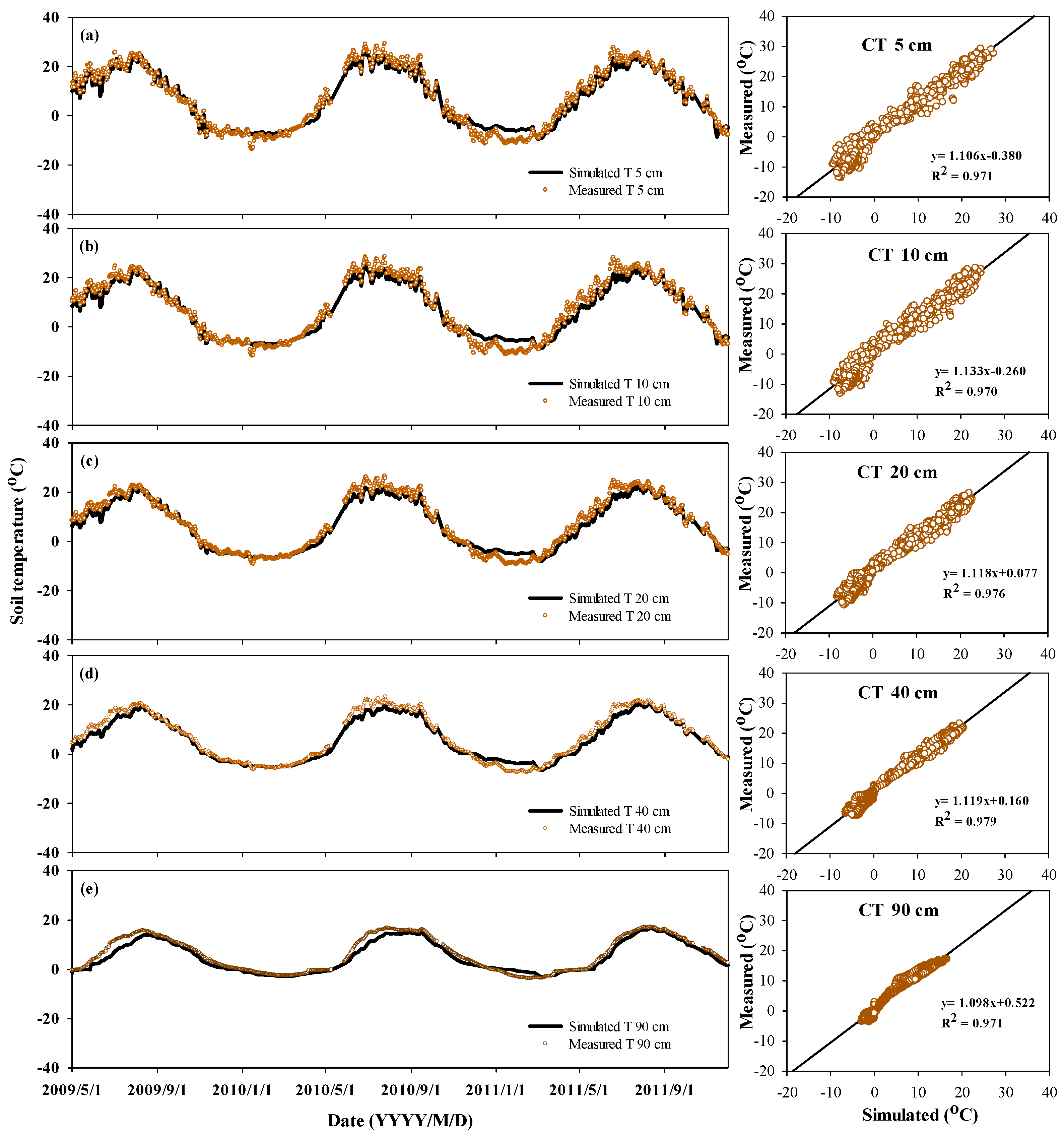
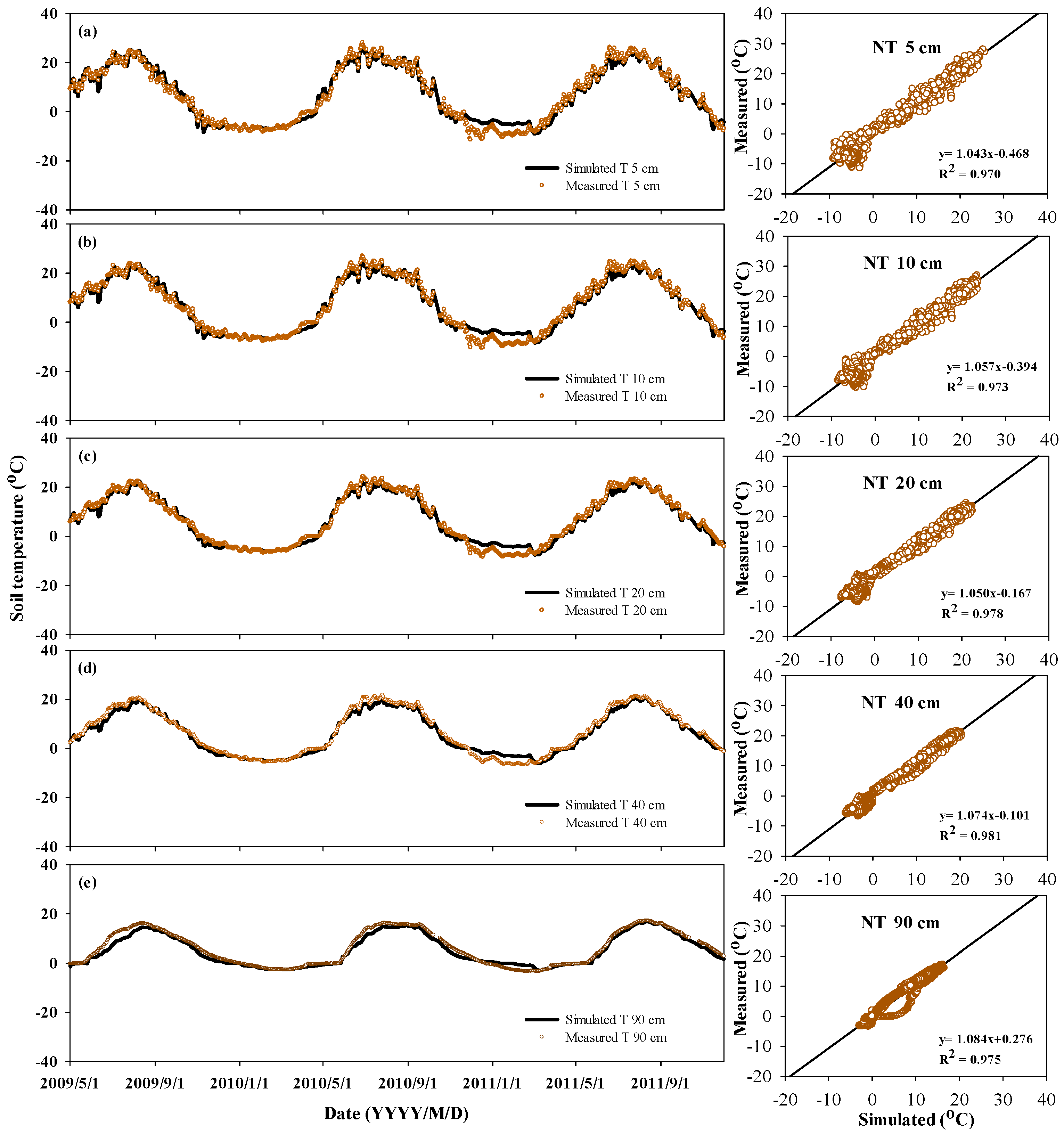
3.1.1. Soil Temperature

The measured and simulated soil temperatures at different soil depths, i.e., 5 cm, 10 cm, 20 cm, 40 cm, and 90 cm, under CT and NT are presented in Figure 1 and Figure 2, respectively. The soil temperature for CT and NT showed similar seasonal fluctuations from year to year during 2009–2011, in response to changes in meteorological conditions (Figure 1). The measured mean soil temperatures for NT were 0.04 °C to 0.27 °C lower compared with CT in all soil depths (Figure 2 and Figure 3; Table S2). It is because NT with crop residue covering the soil surface improved the albedo and reduced the net radiation to the soil surface, especially during the spring and winter seasons. Some studies conducted in the same high latitude regions also reported that NT would lower soil temperature especially in the spring season [12,38,39]. In addition, the amplitudes of the measured soil temperatures for both CT and NT treatments decreased as the soil depths increased (Figure 2 and Figure 3). These results coincide with other research findings [8,40,41].

For model calibration using the CT treatment, the soil temperatures were well simulated by the model at all soil depths, as indicated by the statistics: R² values were equal to 0.97 or 0.98, the nRMSE values ranged from 27.5% to 38.7%, and −1.02 °C ≤ ME ≤ −0.31 °C (Figure 2; Table S2). The measured soil temperatures were consistently underestimated by the model as evidenced by the negative ME values in all soil depths (Figure 2, Table S2), but they were not significantly different from zero according to paired t tests. These results suggest that the model parameters (Table S2) related to the soil heat flow were successfully calibrated under CT treatment. Hence, the CoupModel was considered sufficiently accurate to predict soil temperatures in all soil depths during the years 2009–2011 under CT treatment. The pronounced temperature patterns, not only the overall spatial patterns but also the temporal patterns for soil temperature from 2009 to 2011, were successfully simulated by the model, but the model generally underestimated the measured soil temperatures. The CoupModel prediction levels for the soil temperatures obtained in this study are generally comparable with those in other simulation studies [3,42].

Model evaluation using the NT soil temperature produced higher R² values (≥0.97) and lower nRMSE values (22.8% ≤ nRMSE ≤ 30.6%), indicating better agreements between the simulated and measured soil temperatures relative to CT (Figure 3; Table S2). However, in this case, the corresponding ME values were 0.17 °C and 0.01 °C for 5 cm and 10 cm soil depths, but −0.16 °C, −0.35 °C, and −0.71 °C for 20 cm, 40 cm, and 90 cm depths, respectively, indicating underestimated surface soil temperatures and lower model underestimations in the deeper soil depths for NT relative to CT, although no significant statistical difference was found according to the paired t test (Figure 3; Table S2). Based upon our previous study results on the parameter sensitivity analysis, parameters governing soil thermal conductivity (ClayUnFrozenC1 and ClayFrozenC3) and heat exchange fluxes (CFrozenMaxDamp) need to be further improved, especially during the freeze-thaw period [3], therefore, these parameters were selected in this study to calibrate. It is worth noting that although the soil temperatures in 5 cm, 10 cm, 20 cm, 40 cm, and 90 cm soil depths were overestimated for both treatments during the period from November of 2010 to February of 2011 (Figure 2 and Figure 3), less uncertainty was found than the previous study [3]. It implies that maybe some critical parameters that influence the soil heat processes in the soil freezing period were still not considered in calibration or these parameters were not fully calibrated.

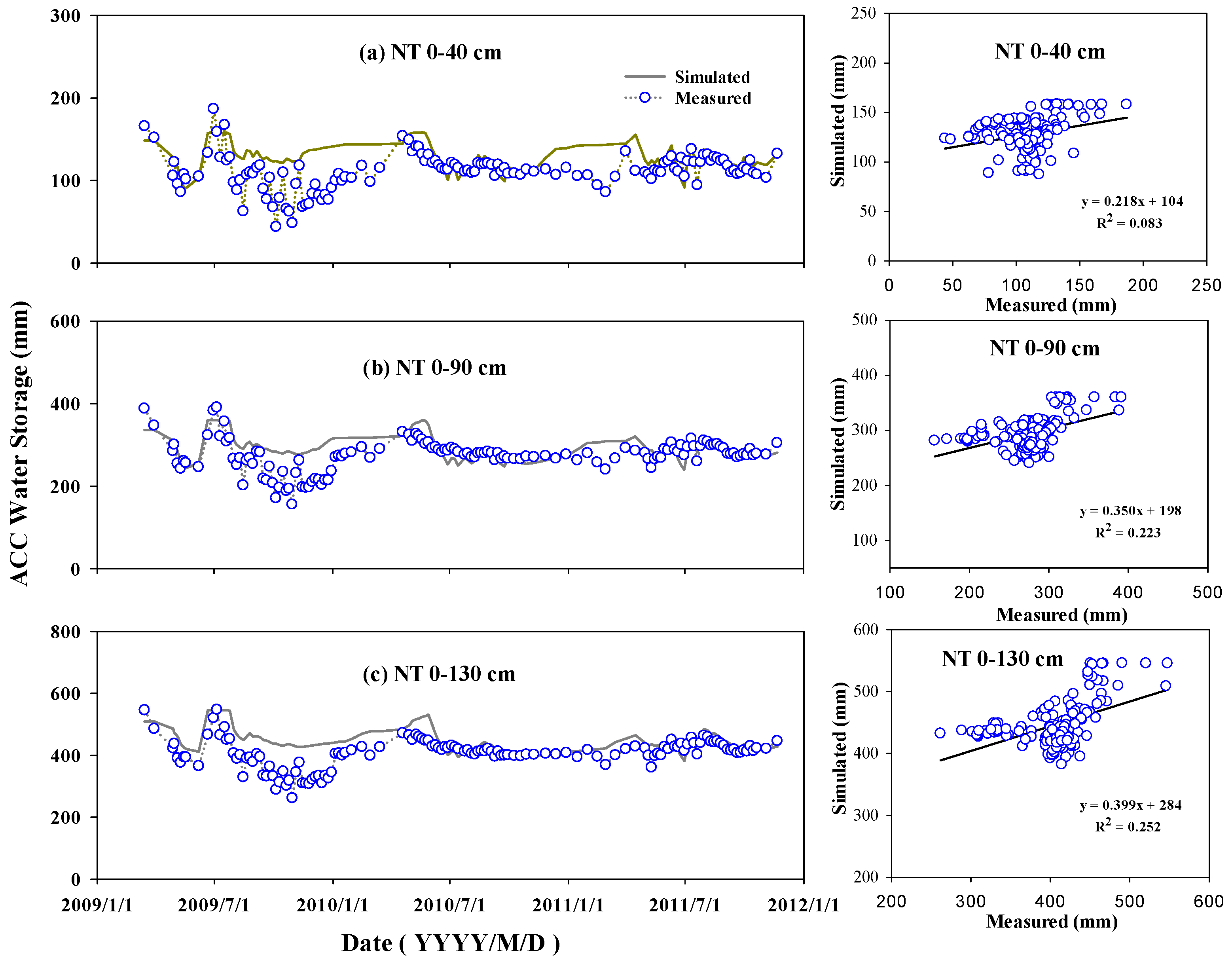
3.1.2. Soil Water Storage

The measured and simulated soil water storage (SWS) data in the time series dynamics during 2009–2011 for CT and NT are shown in Figure 4 and Figure 5. The SWS of 0–40 cm, 0–90 cm, and 0–130 cm demonstrated the dynamics mainly in response to precipitation variations from April to October during 2009–2011. The variation patterns depend on both the annual precipitation and tillage practices (Figure 1). The measured and simulated variation trends are similar for both tillage practices. The measured mean SWS data for CT were 99.9 mm, 255.2 mm, and 383.6 mm in the 0–40 cm, 0–90 cm, and 0–130 cm soil depths, respectively, which were 10%, 7%, and 6% lower than those measured under the NT treatment (Table S2). Especially, the SWS data for NT were much higher than those for CT in both the beginning (January to April) and end (mid-November to December) of the year. Similar results were found by Karunatilake et al. [43] and Wang et al. [44]. Nevertheless, in the wetter months of June and July, no significant differences were found between the two tillage practices (Figure 4 and Figure 5). Wetter soil under NT compared with CT was also found by other authors, especially in the crop root zone soil layer [10,45,46,47,48]. On the one hand, it is due to NT treatment without soil disturbance which can reduce the soil evaporation. On the other hand, the soil surface for NT covered with crop residue improved the albedo and reduced the net radiation to the soil surface, then reduced the soil evaporation [8,41], especially during the spring and winter seasons. Fabrizzi et al. [49] also reported that the increase in soil water storage under NT could be attributed to the increase in infiltration, decrease in evaporation, and enhanced soil protection from rainfall impact.

For the CT treatment used for the model calibration, low R² values (ranging from 0.01 to 0.06) indicated the soil water storage varied trends were not simulated well over the three soil layers. This is due to not only the model predicted error but also the low sampling numbers (n = 142) which increase the uncertainty of the measured curve (Figure 4; Table S2). However, the nRMSE values were 22.6% and 19.6% in 0–90 cm and 0–130 cm soil depths, respectively, indicating that “moderate” agreements between the simulated and measured data were achieved, however, somewhat large variability was found in the 0–40 cm soil depth according to the nRMSE value which is equal to 37.1%. The model tended to overestimate the measured soil water storage, according to the corresponding ME values which were positive (13.3 mm ≤ ME ≤ 28.2 mm).

For model evaluation using the soil water storage data under NT treatment, a better temporal changed curve between the simulated and measured data was achieved, as evidenced by the R² values (0.09 ≤ R² ≤ 0.25) relative to CT. The nRMSE value of 26.0% indicated a “moderate” agreement between the simulated and measured soil water data at 0–40 cm soil depth. The smaller nRMSE values (<15.0%) at both 0–90 cm and 0–130 cm soil depths demonstrated that “good” agreements between the simulated and measured soil water storage were acquired (Figure 5; Table S2). Although the parameters of MinmumCondValue, FreezepointFWi, EquilAdjustPsi, MaxSurfDeficit, MaxSurfExcess, and WindLessExchangeSoil, etc., that are highly responsible for the goodness of fit to the soil water simulations were selected to be calibrated based on the previous sensitivity analysis [3], all positive ME values (18.1 mm ≤ ME ≤ 40.1 mm) proved that the model tended to overestimate the soil water storage at all soil depths. However, less uncertainty was found compared with the previous study [3]. The high ME values for soil and water storage might be caused primarily by the low measurements coinciding with the high simulated soil water storage from the 2009 autumn period to the 2010 spring period (Figure 4 and Figure 5). Overall, the relative differences in water storage intertillage were well predicted by the model (Table S2), although the simulated water storage values were often somewhat larger than the corresponding measured values for both tillage treatments.

3.2. Model Applying

3.2.1. Soil Surface Heat Balance

The heat balances for CT and NT treatments shown in Figure 6 were generated from a single simulation using the parameters calibrated for the CT and NT treatments, respectively (Table S2). Similar varied trends of simulated net radiation (Rn) for CT and NT were found during 2009–2011, both increasing from January then decreasing gradually. The maximum values appeared in June or July, and the minimum values appeared in December (Figure 6a). In general, the simulated Rn for CT was equal to or slightly higher than those for NT.

The latent heat flux (LE), sensible heat flux (H), and surface heat flux (G) are three partitioning fluxes of net radiation (Rn). They varied similarly for CT and NT treatments during the 3 years (Figure 6). The monthly latent heat flux (LE) of CT and NT treatments varied seasonally like the patterns of the net radiation (Rn) in 2009–2011 (Figure 6b). The seasonal variability in monthly LE showed different patterns among the 3 years, partly because of the different seasonal patterns of precipitation (Figure 1). The maximum LE values also appeared in June or July, 104 W M⁻² and 92 W M⁻² in July for CT and NT, respectively, during 2009, 95 W M⁻² and 102 W M⁻² in June for CT and NT, respectively, during 2010, while the maximum LE values appeared in July (94 W M⁻²) and June (83 W M⁻²) for CT and NT, respectively, during 2011. The low values appeared from November to March of the following year for both treatments (Figure 6b). The annual LE for CT varied from 47.5 W m⁻² in 2011 to 43.7 W m⁻² in 2010, resulting from the decrease in annual precipitation and annual soil water storage. However, the annual LE for NT showed lower variations with the values of 40.6 W m⁻², 41.6 W m⁻², and 43.2 W m⁻² for 2009, 2010, and 2011 years, respectively, which may be mainly due to the no-tillage practice which improved the soil water storage. Nevertheless, the sensible heat flux (H) varied differently from LE. The lowest negative values were founded in response to the highest values of LE from April to October of all three years, while the highest positive values of H appeared from November to March in response to the lowest values of LE for both treatments (Figure 6b). The soil heat flux (G) varied similarly from 2009 to 2011. Generally, the G values for CT and NT treatments showed positive values ranging from 4.5 W M⁻² to 30.1 W M⁻², as a net sink, from April to August during 2009–2011. The monthly G values for CT were equal to or slightly higher than those for NT treatment during 2009–2011 (Figure 6c).

3.2.2. Root Zone Soil Water Dynamics

The soil water contents in the crop root zone are crucial for crop seed emergence and crop early growth, especially in the arid and semi-arid agricultural area where the precipitation varies seasonally and annually. Figure 7a presents the simulated average volumetric soil water contents at 0–10 cm depth under CT and NT treatments from 2009 to 2011. The soil water contents for both treatments followed the similar varied trend characterized by low soil water contents in winter which is because rare precipitation (in the form of snow) infiltrated into the soil profile due to the soil frost. In general, the differences between the NT and CT treatments were most visible in the root zone soil water contents, more under NT than CT during the rainfall season (from May until October), especially during the crop planting time in spring (May) and the crop harvest time in autumn (October). In addition, the soil water contents showed similar values for both tillage treatments during winter time (from November until March) (Figure 7a). Similar results were reported by other researchers [47,48].

3.2.3. Soil Evaporation

Figure 7b shows that the simulated soil evaporation curves for CT and NT treatments had similar varied trends over 2009–2011. The soil evaporation amounts for CT treatment, in general, were greater in contrast with NT treatment over the three years. No soil evaporation was found from mid-November to mid-April of the following year. This is due to the lower air temperatures during the winter time when the soil was under frost condition (Figure 7b), while most soil evaporation occurred during the corresponding unfrosted period for both treatments (Figure 7b). The total accumulated soil evaporation for NT was 1414 mm, which was 113 mm lower than that for CT treatment during 2009–2011. Since no-tillage operations were applied for NT treatment with the crop residue covering the soil surface, both the operations and the crop residue could reduce the soil evaporation [10] through varying soil surface energy balance [50] and increasing the rainfall infiltration into soil [51], thus transporting more water to deeper soil layers. The total accumulated soil evaporation for NT was 62 mm lower than CT in 2009, accounting for 55 percent of the total lower soil evaporation (113 mm) during the three years, while it was 12 mm and 39 mm lower in 2010 and 2011, respectively (Figure 7b).

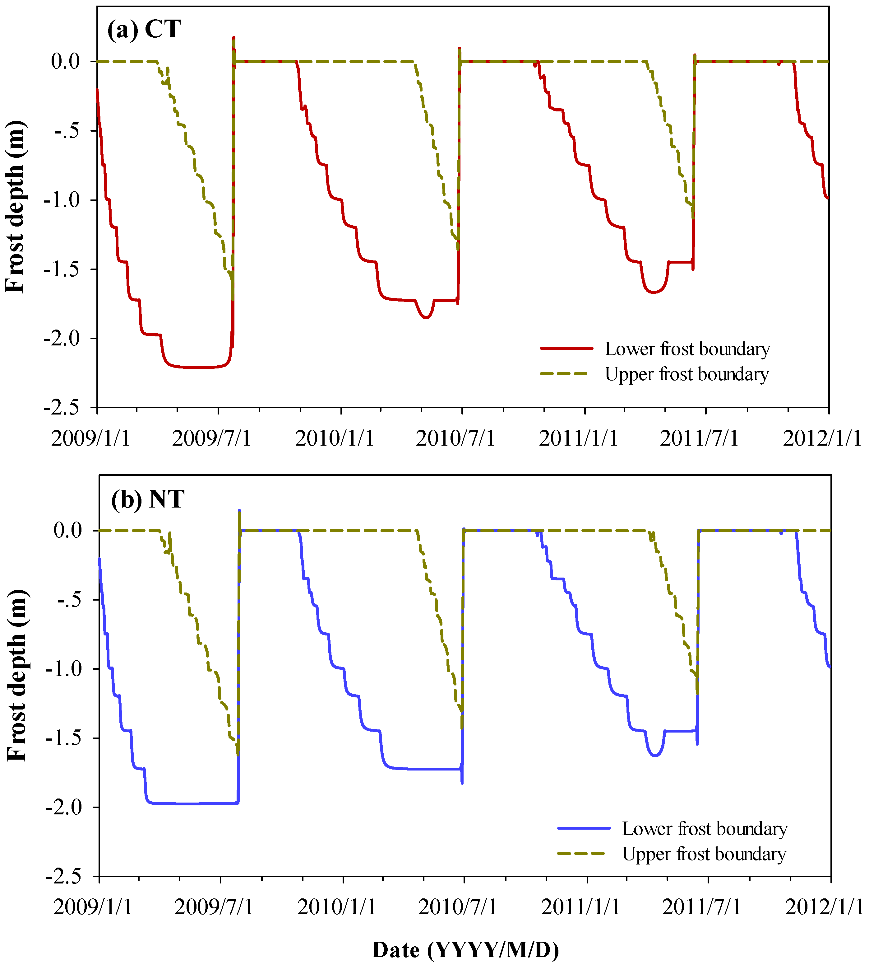
3.2.4. Soil Frozen Depth Dynamics

As the soil frozen depths dynamics were influenced by both soil temperature and soil water, after the model calibration and evaluation used measured soil temperature and soil water storage data, the soil frozen depth dynamical curves under CT and NT treatment were reproduced by the calibrated CoupModel. The simulated frost depth showed realistic frost depth values during the freezing and thawing periods as the soil started to freeze at the end of October and then gradually went down to the deepest depths for both CT and NT treatments (Figure 8). The mean annual freezing period is usually from the end of October to mid-April of the following year, while the mean annual thawing period is normally from the beginning of April to the end of June for both treatments. Hence, more than 50% of the whole year is in freeze–thaw environments, and the soil physical characteristics change seasonally, which could increase the uncertainty of estimating suitable parameters by the model. The lower frost boundary showed more variability than the upper frost boundary. The lowest frozen depths were 2.21 m, 1.85 m, and 1.67 m below the soil surface for CT in 2009, 2010, and 2011, respectively (Figure 8a). However, NT showed lower values compared with CT, with the lowest frozen depths being 1.98 m, 1.73 m, and 1.63 m below the soil surface in 2009, 2010, and 2011, respectively (Figure 8b). The frozen depths were similar to the values (1.77 m to 2.77 m) reported by Wu et al. [3] in the same research region in China. The simulated average thawing rate was approximately 2.1 cm day⁻¹, which was similar to the estimated values reported by Zhang et al. [52] in the same region of China (2.1–2.4 cm day⁻¹).

3.2.5. Problem and Deficit in Calibration and Evaluation Processes

The soil water and temperatures in different soil layer depths under CT were used in the calibration process. The calibrated parameters and their feasible ranges were chosen according to our experience and literature in this Mollisols region. Most of the parameters adopted the default values from previous applications of the model. Therefore, the main deficits of the calibration might be that (i) the chosen parameters were insufficient, and some critical parameters that influence the soil water and heat processes were still not considered in calibration or these parameters were not fully calibrated. In addition, some of the default parameter values inside the model that were directly used in this study might be not suitable or accurate enough. (ii) The soil hydraulic parameters measured under CT (Table 1) were used as input values at the begin of the modeling, however, the soil hydraulic parameters could be changed intra- and inter-annually mainly due to the field management (Table 2), especially the three-time tillage, yearly. (iii) The soil heat transfer parameters (Table S1) were calibrated in this study due to the difficulty of measuring, and these parameters could also be changed intra- and inter-annually by frequent tillage. In the evaluation process using the measured soil water and temperature data under NT, the main deficits of the evaluation might be from the crop straw cover in the soil surface for NT; the crop straw cover was not fully considered in the model, and thus no specified crop straw cover parameters can be set up as input. So the parameter of albedo dry was set 5% higher than that for CT, and RoughLBareSoilMom (surface roughness length for momentum above bare soil) was set twice as high as that for CT according to our experience and previous studies.

It is worth noting that the simulated soil temperatures were lower than the measurements in 5 cm, 10 cm, 20 cm, 40 cm, and 90 cm soil depths during the period of April to July for CT (not for NT) (Figure 2 and Figure 3). This might be due to the deficits in some soil heat transfer parameters that might be changed by tillage that usually operated during April to July for CT (Table 2), which was not fully considered by the model. The simulated soil temperatures were higher than the measurements in 5 cm, 10 cm, 20 cm, 40 cm, and 90 cm soil depths during the period of December of 2010 to February of 2011 for both CT and NT, but did not appear during the winter period of 2009 to 2010 (Figure 2 and Figure 3), which implies that some parameters influencing soil heat processes under soil freezing conditions need to be carefully calibrated, for example, the parameter of snow depth (0.18 m) in this study was only measured during the winter period of 2009 as initial input data, but not during the winter period of 2010 to 2011, so we recommend measuring snow depth during each winter period in further studies. The soil water storage values were overestimated by the model mainly during the freeze–thaw periods (October to April of the following year) for both CT and NT (Figure 4 and Figure 5), which might be due to the deficits of some parameters as a result of soil water processes not being considered in calibration or were not fully calibrated. Therefore, parameters need to be more carefully considered during the freeze–thaw periods in future studies.

4. Conclusions

The model parameters were successfully calibrated with the field measurements of daily soil temperatures and soil water storage in different soil depths from the CT system, proven by the soil temperatures and water storage which were well simulated by the model at all soil depths. For NT tillage systems for the model evaluation, the CoupModel provided “moderate to good agreements” between simulated and measured soil temperature. Overall, the temporal and spatial variations of soil temperature and water were successfully predicted by the CoupModel. The soil temperatures in all soil depths were overestimated for both tillage systems during the period from November of 2010 to February of 2011, which is attributed to some critical parameters that influenced the soil heat processes in the soil freezing period. These parameters were not considered in calibration or were not fully calibrated. It was concluded that the CoupModel proved to be a functional tool to predict soil heat and water processes for CT and NT systems in the cool, semiarid, and high-latitude seasonal frost conditions of Mollisols in northeast China. The model estimated the soil temperature, water, soil energy balance, and frost depth dynamics in relatively complex systems that combined plant dynamics with tillage and/or no tillage covered with crop straw mulching in the soil surface. The results of this study are valuable for testing the ability of the CoupModel and increasing our understanding of soil heat and water processes. For further research on the freeze–thaw process, consideration of the uncertainty caused by snow properties and measurements on soil water during the winter time are suggested.

References

1. Liu, X.B.; Han, X.Z.; Herbert, S.J.; Xing, B. Soil organic carbon dynamics in Black soils of China under different agricultural management systems. Commun. Soil Sci. Plant. Anal. 2003, 34, 973–984. [Google Scholar] [CrossRef]
2. Xu, X.Z.; Xu, Y.; Chen, S.C.; Xu, S.G.; Zhang, H.W. Soil loss and conservation in the black soil region of northeast China: A retrospective study. Environ. Sci. Policy 2010, 13, 793–800. [Google Scholar] [CrossRef]
3. Wu, S.H.; Jansson, P.E.; Zhang, X.Y. Modelling temperature, moisture and surface heat balance in bare soil under seasonal frost conditions in China. Eur. J. Soil Sci. 2011, 62, 780–796. [Google Scholar] [CrossRef]
4. Hassanili, A.M.; Ebrahimizadeh, M.A.; Beecham, S. The effects of irrigation methods with effluent and irrigation scheduling on water use efficiency and corn yields in an arid region. Agric. Water Manag. 2009, 96, 93–99. [Google Scholar] [CrossRef]
5. Wang, Y.J.; Xie, Z.K.; Sukhdev, S.M.; Cecil, L.V.; Zhang, Y.B.; Guo, Z.H. Effects of gravel–sand mulch, plastic mulch and ridge and furrow rainfall harvesting system combinations on water use efficiency, soil temperature and watermelon yield in a semi-arid loess plateau of Northwestern China. Agric. Water Manag. 2011, 101, 88–92. [Google Scholar] [CrossRef]
6. Zhang, S.L.; Zhang, X.Y.; Huffman, T.; Liu, X.B.; Yang, J.Y. Influence of topography and land management on soil nutrients variability in Northeast China. Nutr. Cycl. Agroecosyst. 2011, 89, 427–438. [Google Scholar] [CrossRef]
7. Liu, X.B.; Jin, J.; Wang, G.H.; Herbert, S.J. Soybean yield physiology and development of high-yielding practices in Northeast China. Field Crops Res. 2008, 105, 157–171. [Google Scholar] [CrossRef]
8. Chen, Y.; Liu, S.; Li, H.; Li, X.F.; Song, C.Y.; Cruse, R.M.; Zhang, X.Y. Effects of conservation tillage on corn and soybean yield in the humid continental climate region of Northeast China. Soil Tillage Res. 2011, 116, 56–61. [Google Scholar] [CrossRef]
9. Puustinen, M.; Koskiaho, J.; Peltonen, K. Influence of cultivation methods on suspended solids and phosphorus concentrations in surface runoff on clayey sloped fields in boreal climate. Agric. Ecosyst. Environ. 2005, 105, 565–579. [Google Scholar] [CrossRef]
10. Schwartz, R.C.; Baumhardt, R.L.; Evett, S.R. Tillage effects on soil water redistribution and bare soil evaporation throughout a season. Soil Tillage Res. 2010, 110, 221–229. [Google Scholar] [CrossRef]
11. Campbell, C.A.; Biederbeck, V.O.; Schnitzer, M.; Selles, F.; Zentner, R.P. Effect of 6 years of zero tillage and fertilizer management on changes in soil quality of an orthicbrown chernozem in Southwestern Saskatchewan. Soil Tillage Res. 1989, 14, 39–52. [Google Scholar] [CrossRef]
12. Drury, C.F.; Tan, C.S.; Welacky, T.W.; Oloya, T.O.; Hamill, A.S.; Weaver, S.E. Red clover and tillage influence on soil temperature, water content, and corn emergence. Agron. J. 1999, 91, 101–108. [Google Scholar] [CrossRef]
13. Khaledian, M.R.; Mailhol, J.C.; Ruelle, P.; Rosique, P. Adapting pilote model for water and yield management under direct deeding system: The case of corn and durum wheat in a Mediterranean context. Agric. Water Manag. 2009, 96, 757–770. [Google Scholar] [CrossRef] [Green Version]
14. Flerchinger, G.N.; Hardegree, S.P. Modelling near-surface soil temperature and moisture for germination response predictions of post-wildfire seedbeds. J. Arid Environ. 2004, 59, 369–385. [Google Scholar] [CrossRef]
15. Whisler, F.D.; Acock, B.; Baker, D.N.; Fye, R.E.; Hodges, H.F.; Lambert, J.R.; Lemmon, H.E.; McKinion, J.M.; Reddy, V.R. Crop simulation models in agronomic systems. Adv. Agron. 1986, 40, 141–208. [Google Scholar] [CrossRef]
16. Bouman, B.A.M.; van Keulen, H.; van Laar, H.H.; Rabbinge, R. The ‘school of de wit’ crop growth simulation models: A pedigree and historical overview. Agric. Syst. 1996, 52, 171–198. [Google Scholar] [CrossRef]
17. Brisson, N.; Gary, C.; Justes, E.; Roche, R.; Mary, B.; Ripoche, D.; Zimmer, D.; Sierra, J.; Bertuzzi, P.; Burger, P.; et al. An overview of the crop model STICS. Eur. J. Agron. 2003, 18, 309–332. [Google Scholar] [CrossRef]
18. Saito, H.; Šimůnek, J. Effects of meteorological models on the solution of the surface energy balance and soil temperature variations in bare soils. J. Hydrol. 2009, 373, 545–561. [Google Scholar] [CrossRef]
19. Flerchinger, G.N.; Pierson, F.B. Modeling plant canopy effects on variability of soil temperature and water. Agricult. Forest Meterol. 1991, 56, 227–246. [Google Scholar] [CrossRef]
20. Flerchinger, G.N.; Sauer, T.J.; Aiken, R.A. Effects of crop residue cover and architecture on heat and water transfer at the soil surface. Geoderma 2003, 116, 217–233. [Google Scholar] [CrossRef]
21. Ji, X.B.; Kang, E.S.; Zhao, W.Z.; Zhang, Z.H.; Jin, B.W. Simulation of heat and water transfer in a surface irrigated, cropped sandy soil. Agric. Water Manag. 2009, 96, 1010–1020. [Google Scholar] [CrossRef]
22. Mailhol, J.C.; Olufayo, A.A.; Ruelle, P. Sorghum and sunflower evapotranspiration and yield from simulated leaf area index. Agric. Water Manag. 1997, 35, 167–182. [Google Scholar] [CrossRef]
23. Jansson, P.E.; Moonb, D.S. A coupled model of water, heat and mass transfer using object orientation to improve flexibility and functionality. Environ. Modell Softw. 2001, 16, 37–46. [Google Scholar] [CrossRef]
24. Zhang, S.L.; Lövdahl, L.; Grip, H.; Jansson, P.E.; Tong, Y.N. Modelling the effects of mulching and fallow cropping on water balance in the Chinese loess plateau. Soil Tillage Res. 2007, 93, 283–298. [Google Scholar] [CrossRef]
25. Beven, K.J.; Binley, A. The future of distributed models: Model calibration and uncertainty prediction. Hydro. Process 1992, 6, 279–298. [Google Scholar] [CrossRef]
26. Jansson, P.E.; Karlberg, L. CoupModel-coupled heat and mass transfer model for soil–plant–atmosphere system. In TRITA-LWR Report, 3087; Royal Institute of Technology, Department of Land and Water Resources Engineering: Stockholm, Sweden, 2004; p. 427. [Google Scholar]
27. Wu, S.H.; Jansson, P.E.; Kolari, P. Modeling seasonal course of carbon fluxes and evapotranspiration in response to low temperature and moisture in a boreal Scots pine ecosystem. Ecol. Model. 2011, 222, 3103–3119. [Google Scholar] [CrossRef]
28. Beck, H.E.; Zimmermann, N.E.; McVicar, T.R.; Vergopolan, N.; Berg, A.; Wood, E.E. Publisher Correction: Present and future Köppen-Geiger climate classification maps at 1-km resolution. Sci. Data 2020, 7, 274. [Google Scholar] [CrossRef] [PubMed]
29. Jansson, P.E.; Halldin, S. Model for the annual water and energy flow in a layered soil. In Comparison of Forest and Energy Exchange Models; Halldin, S., Ed.; Society for Ecological Modelling: Copenhagen, Denmark, 1979; pp. 145–163. [Google Scholar]
30. Eckersten, H.; Jansson, P.E.; Johnsson, H. SOILN Model, Version 9.2, User’s Manual. Division of Hydrotechnics; Swedish Agricultural University: Uppsala, Sweden, 1998. [Google Scholar]
31. Monteith, J.L. Evaporation and environment. In The State and Movement of Water in Living Rrganisms, Proceedings of the 19 Symposium of Society of Experimental Biology, Swansea, 1964; Fogg, G.E., Ed.; The Company of Biologists: Cambridge, UK, 1965; pp. 205–234. [Google Scholar]
32. Jansson, P.E. CoupModel: Model use, calibration, and validation. Trans. ASABE 2012, 55, 1335–1344. [Google Scholar] [CrossRef]
33. Richards, L.A. Capillary conduction of liquids through porous media. Physics 1931, 1, 318–333. [Google Scholar] [CrossRef]
34. Brooks, R.H.; Corey, A.T. Hydrological Properties of Porous Media; Hydrology Paper No. 3; Colorado State University: Fort Collins, CO, USA, 1964. [Google Scholar]
35. Mualem, Y. A new model for predicting the hydraulic conductivity of unsaturated porous media. Water Resour. Res. 1976, 12, 513–522. [Google Scholar] [CrossRef] [Green Version]
36. Liu, S.; Yang, J.Y.; Drury, C.F.; Liu, H.L.; Reynolds, W.D. Simulating maize (Zea mays L.) growth and yield, soil nitrogen concentration, and soil water content for a long-term cropping experiment in Ontario, Canada. Can. J. Soil Sci. 2014, 94, 435–452. [Google Scholar] [CrossRef]
37. Liu, S.; Yang, J.Y.; Yang, X.M.; Drury, C.F.; Jiang, R.; Reynolds, W.D. Simulating maize yield at county scale in southern Ontario using the decision support system for agrotechnology transfer model. Can. J. Soil Sci. 2021, 101, 734–748. [Google Scholar] [CrossRef]
38. Sarkar, S.; Singh, S.R. Interactive effect of tillage depth and mulch on soil temperature, productivity and water use pattern of rainfed barley (Hordium vulgare L.). Soil Tillage Res. 2007, 92, 79–86. [Google Scholar] [CrossRef]
39. Soane, B.D.; Ball, B.C.; Arvidsson, J.; Basch, G.; Moreno, F.; Roger-Estrade, J. No-till in northern, western and south-western Europe: A review of problems and opportunities for crop production and the environment. Soil Tillage Res. 2012, 118, 66–87. [Google Scholar] [CrossRef] [Green Version]
40. Chassot, A.; Stamp, P.; Richner, W. Root distribution and morphology of maize seedlings as affected by tillage and fertilizer placement. Plant Soil. 2001, 231, 123–135. [Google Scholar] [CrossRef]
41. Sommer, R.; Wall, P.C.; Govaerts, B. Model-based assessment of maize cropping under conventional and conservation agriculture in highland Mexico. Soil Tillage Res. 2007, 94, 83–100. [Google Scholar] [CrossRef]
42. Rasmussen, L.H.; Zhang, W.X.; Hollesen, J.; Cable, S.; Christiansen, H.H.; Jansson, P.E.; Elberling, B. Modelling present and future permafrost thermal regimes in Northeast Greenland. Cold Reg. Sci. Technol. 2018, 146, 199–213. [Google Scholar] [CrossRef]
43. Karunatilake, U.; van Es, H.M.; Schindelbeck, R.R. Soil and maize response to plow and no-tillage after alfalfa-to-maize conversion on a clay loam soil in New York. Soil Tillage Res. 2000, 55, 31–42. [Google Scholar] [CrossRef]
44. Wang, X.B.; Dai, K.; Zhang, D.C.; Zhang, X.M.; Wang, Y.; Zhao, Q.S.; Cai, D.X.; Hoogmoed, W.B.; Oenema, O. Dryland maize yields and water use efficiency in response to tillage/crop stubble and nutrient management practices in China. Field Crops Res. 2011, 120, 47–57. [Google Scholar] [CrossRef]
45. Su, Z.Y.; Zhang, J.S.; Wu, W.L.; Cai, D.X.; Lv, J.J.; Jiang, G.H.; Huang, J.; Gao, J.; Hartmann, R.; Gabriels, D. Effects of conservation tillage practices on winter wheat water-use efficiency and crop yield on the loess plateau, China. Agric. Water Manag. 2007, 87, 307–314. [Google Scholar] [CrossRef]
46. Alvarez, R.; Steinbach, H.S. A review of the effects of tillage systems on some soil physical properties, water content, nitrate availability and crops yield in the Argentine Pampas. Soil Tillage Res. 2009, 104, 1–15. [Google Scholar] [CrossRef]
47. Sharma, P.; Abrol, V.; Sharma, R.K. Impact of tillage and mulch management on economics, energy requirement and crop performance in maize-wheat rotation in rainfed subhumid inceptisols, India. Eur. J. Agron. 2011, 34, 46–51. [Google Scholar] [CrossRef]
48. Cullum, R.F. Influence of tillage on maize yield in soil with shallow fragipan. Soil Tillage Res. 2012, 119, 1–6. [Google Scholar] [CrossRef]
49. Fabrizzi, K.P.; García, F.O.; Costa, J.L.; Picone, L.I. Soil water dynamics, physical properties and corn and wheat responses to minimum and no-tillage systems in the southern Pampas of Argentina. Soil Tillage Res. 2005, 81, 57–69. [Google Scholar] [CrossRef]
50. Horton, R.; Bristow, K.L.; Kluitenberg, G.J.; Sauer, T.J. Crop residue effects on surface radiation and energy balance—Review. Theor. Appl. Climatol. 1996, 54, 27–37. [Google Scholar] [CrossRef] [Green Version]
51. Liu, S.; Zhang, X.Y.; Kravchenko, Y.; Iqbal, M.A. Maize (Zea mays L.) yield and soil properties as affected by no tillage in the black soils of China. Acta Agric. Scand. B Soil Plant Sci. 2015, 65, 554–565. [Google Scholar] [CrossRef]
52. Zhang, S.L.; Lövdahl, L.; Grip, H.; Tong, Y.N.; Yang, X.Y.; Wang, Q.J. Effects of mulching and catch cropping on soil temperature, soil moisture and wheat yield on the loess plateau of China. Soil Tillage Res. 2009, 102, 78–86. [Google Scholar] [CrossRef]
Figure 1. Daily precipitation and average air temperature from 2009 to 2011.
Land 11 00417 g001
Figure 2. Simulations vs. measurements of daily soil temperatures at (a) 5 cm, (b) 10 cm, (c) 20 cm, (d) 40 cm, and (e) 90 cm for CT during 2009–2011.
Land 11 00417 g002
Figure 3. Simulations vs. measurements of daily soil temperatures at (a) 5 cm, (b) 10 cm, (c) 20 cm, (d) 40 cm, and (e) 90 cm for NT during 2009–2011.
Land 11 00417 g003
Figure 4. Simulations vs. measurements of water storage at (a) 0–40 cm, (b) 0–90 cm, and (c) 0–130 cm for CT during 2009–2011.
Land 11 00417 g004
Figure 5. Simulations vs. measurements of water storage at (a) 0–40 cm, (b) 0–90 cm, and (c) 0–130 cm for NT during 2009–2011.
Land 11 00417 g005
Figure 6. Simulated monthlysoil heat fluxes (a) LE, H and (c) G and (b) net radiation for CT and NT during 2009–2011.
Land 11 00417 g006
Figure 7. Simulated (a) daily average soil water contents at 0–10 cm depth and (b) daily soil evaporation for CT and NT during 2009–2011.
Land 11 00417 g007
Figure 8. Simulated upper and lower boundaries of frost depth for (a) and (b) during 2009–2011.
Land 11 00417 g008