Article

Mapping Agricultural Lands: From Conventional to Regenerative

1
Department of Geography, University of British Columbia, 1984 West Mall–Rm 217, Vancouver, BC V6T 1Z2, Canada
2
Instituto Conmemorativo Gorgas de Estudios de la Salud, Ciudad de Panamá 0816-02593, Panama
3
Midwest Healthy Ag, 6771 South Silver Hill Dr., Finland, MN 55603, USA
4
Agroecology and Rural Economics Research Corps, 1439 Grand Ave., Saint Paul, MN 55105, USA
*
Author to whom correspondence should be addressed.
Land 2022, 11(3), 437; https://doi.org/10.3390/land11030437
Submission received: 17 February 2022 / Revised: 11 March 2022 / Accepted: 14 March 2022 / Published: 17 March 2022
(This article belongs to the Section Land Socio-Economic and Political Issues)

Abstract

:
In an era in which conventional agriculture has come under question for its environmental and social costs, regenerative agriculture suggests that land management practices can be organized around farming and grazing practices that regenerate interdependent ecological and community processes for generations to come. However, little is known about the geographies of ‘regenerative’ and ‘conventional’ agricultural lands—what defines them, where they are, and the extent to which actual agricultural lands interweave both or are characterizable by neither. In the context of the Midwest of the United States, we develop and map an index quantifying the degrees to which the agricultural lands of counties could be said to be regenerative, conventional, or both. We complement these results by using a clustering method to partition the land into distinct agricultural regions. Both approaches rely on a set of variables characterizing land we developed through an iterative dialogue across difference among our authors, who have a range of relevant backgrounds. We map, analyze, and synthesize our results by considering local contexts beyond our variables, comparing and contrasting the resulting perspectives on the geographies of midwestern agricultural lands. Our results portray agricultural lands of considerable diversity within and between states, as well as ecological and physiographic regions. Understanding the general patterns and detailed empirical geographies that emerge suggests spatial relationships that can inform peer-to-peer exchanges among farmers, agricultural extension, civil society, and policy formation.

1. Introduction

In focusing on turning natural and social resources into commodities via economies of scale, conventional agriculture has tended to contribute not only to increased outputs but also to widespread socioenvironmental damage [1,2,3,4,5,6]. Agroecology and regenerative agriculture represent systems organized around farming and grazing practices that regenerate interdependent ecological and community processes for generations to come [7,8,9,10,11]. The approaches aim to integrate soil, water, livestock, wildlife, individuals, and communities into interconnected units forming resilient ecosocial assemblages.
For many, regenerative agriculture is focused on developing healthy soil through practices such as cover cropping, intercropping, crop rotation, conservation tillage, and mixed crop–livestock systems [12,13,14,15,16,17]. Other regenerative practices may include wildlife corridors, buffer strips to control runoff, habitat for pollinators, and integrated pest management [18,19,20,21,22,23,24]. The resulting benefits increase regional biodiversity, improve water quality, and enhance ecosystem services, including drought and flood control. Regenerative practices have been documented to improve soil organic carbon and mineral-associated organic matter [25,26]. They also promote landscape resilience to climatic instability [27]. Other studies have shown that regenerative agriculture provides benefits by providing improved nutrient densities in vegetables and wheat, and that regenerative grazing provides a better fatty-acid profile than conventionally raised beef [28].
The discipline and practice of agroecology depend on interventions in community wellbeing and broader political economies that some programs in regenerative agriculture are now beginning to incorporate [29,30,31]. Such approaches aim to reset settler histories that served as the basis of ongoing expropriation disconnecting food production from local ecologies and community life [32,33,34,35]. The interventions aim to reintroduce farmer autonomy, community socioeconomic resilience, circular economies, epidemiological buffering, and integrated cooperative supply networks [36,37]. The approaches aim to institutionalize democratic participatory processes that protect the interdependent health and welfare of farmers, workers, consumers, local communities, livestock and poultry, wildlife, and, by extension, a greater world extending far beyond the farm gate. Re-establishing interwoven regional food systems that can supply produce rich in the diversity and micronutrients lost in industrial production can also remove farmers from the price treadmill, provide seasonally appropriate and healthy food options, and mend the disconnect between rural and urban communities [38,39,40,41,42,43].
Despite these clear distinctions, as a matter of an operational definition usable for mapping, the questions of what forms a regenerative or conventional agricultural land—or where these terms are inadequate—is not simply answered. A nascent literature is beginning to address this question, although still largely in terms of proximate on-farm measures and practices, including soil health, water retention, and farm profits [44,45,46]. There has been research attempting to partition agricultural lands into regions of shared characteristics since at least the early 20th century [47,48,49,50,51], but such inquiry has not differentiated regenerative from what we now call ‘conventional’ practices. It has likewise focused more closely solely on farm practices and biophysical conditions than a broader regenerative agricultural sensibility might suggest. As has been long understood, a set of agricultural regions drawn for one purpose may mislead those who casually use them for another [49].
Our methods consider land as integrative, including but moving beyond the farm and soil health. We do so through developing two complementary approaches to quantifying, visualizing, and analyzing the agricultural lands of the US Midwest—a conventional–regenerative agricultural index whose values vary over space, as well as a partitioning of the land into distinct agricultural regions via a clustering approach. Both rely on a set of variables characterizing the land we developed through an iterative dialogue across differences among our authors, who have a range of relevant backgrounds. While previous studies have focused on characterizing either conventional or regenerative agricultural lands, we begin with the supposition that many regenerative farmers still practice conventional methods, including pesticide use, and many conventional farmers are engaging basic regenerative practices such as cover crops and rotational grazing. We, therefore, design our index and regionalization methods to quantify and map how various places combine conventional and regenerative agricultural practices in similar or different ways and extents.
We map, analyze, and synthesize our results by considering local contexts beyond our variables, comparing and contrasting the resulting perspectives on the geographies of midwestern agricultural lands. Our results portray agricultural lands of considerable diversity within and between states, as well as ecological and physiographic regions. Understanding the general patterns and detailed empirical geographies that emerge suggest spatial relationships that might inform peer-to-peer exchanges among farmers, agricultural extension, civil society, and policy formation.

2. Materials and Methods

Our investigation of regenerative and conventional agricultural lands in the US Midwest began with a collaboration across our differences in standpoints as farmers, food system analysts, and/or academics. We worked to identify which sorts of measurable processes and attributes of the land we can agree are best included in our analysis.
We root our consideration of what constitutes various types of agricultural land in the study of 12 states in the US Midwest, which, listed from east to west, are Ohio, Indiana, Michigan, Wisconsin, Illinois, Missouri, Iowa, Minnesota, North Dakota, South Dakota, Nebraska, and Kansas. Although it is desirable to study such lands at multiple, interconnected scales, we focus here on aggregated data, data that somewhat subsume the actions of the individual into larger landscape processes, but that are not so broad as to suppress all forms of variation from locale to locale or state to state. In doing so, our choice of scale and our choice of data sources are interdependent.
Many of the variables we chose were easily obtainable at the county level, given the format of public data of the USDA’s 2017 Census of Agriculture and other studies upon which we relied. Several of our variables were derived from gridded rasters that we then re-expressed at the county level, as described below, as well as in full detail in the Supplementary Materials. Not all data we used were derived from 2017 measurements, but data were chosen to be as close to 2017 in provenance as possible. Many of the processes captured by the variables we chose (and describe below) do not have large interannual variations in the short term.
After choosing variables (as described in more detail below) that we felt were related to how regenerative and/or conventional agricultural land might be, we then characterized the lands of the US Midwest given these variables. To do so, we developed two approaches with different assumptions and placed their results in conversation with each other, which we describe further below: (1) a single continuous regenerative–conventional agricultural land index via a function using the variables as its parameters; (2) a discrete classification/regionalization of counties via clustering the variables.

2.1. Selecting a Functional Form for a Regenerative–Conventional Agricultural Index

One of the first choices that needed to be made was the functional form for the index. Although any number of forms might be conceivably plausible or insightful for this analysis, we chose to use a ratio in our efforts to compare agricultural lands across the region. In our case, this choice of form allowed for a clear differentiation in the role played by a numerator and a denominator of the ratio. We allow the numerator and denominator to each be a sum of variables, with the numerator’s terms being variables that we felt would be positively associated with regenerative agriculture, whereas the variables in the sum forming the denominator would be negatively associated with regenerative agriculture and positively associated with conventional agriculture. In other words, let
I n d e x = n u m e r a t o r d e n o m i n a t o r ,
where n u m e r a t o r = n X n and d e n o m i n a t o r = m Y m given sets of variables X n and Y m .
A higher value of the ratio in a particular county suggests a greater association of the agriculture of the county with regenerative practices than with conventional ones; a lower value of the index implies more conventional practices, while grounds in the middle represent a balance. Note that the value of the index itself does not necessarily speak to the overall amount of activity in a county compared to other counties, but to the qualitative nature of the activities.

2.2. Exploring, Choosing, and Preparaing Regenerative–Conventional Variables

In the United States, regenerative agriculture is not currently associated with a highly standardized set of activities or outcomes. As authors of this work, we brought insights and aspirations from overlapping experiences as farmers, food systems analysts, natural scientists, and/or social scientists to our understanding of what might comprise both regenerative and conventional agricultural lands. We collaborated across differences to choose variables that would describe and differentiate these agricultural lands across the diversity of the twelve states considered here, ranging from the Appalachian foothills to the Great Plains, from northern forests and lakes to the central lowlands and rolling hills of loess, hosting so many specific practices in husbandry and cultivation. Choosing specialty maple production, for instance, would overemphasize the differences both within certain northern states such as Wisconsin and Michigan and between those states and others. It was important to us that the variables be appropriate to characterizing the land in an integrative fashion; not only on-farm practices but also communitywide social economies and interrelated environmental processes were important to capture. Choosing methane production and particulate matter as markers of conventional production speaks to our interests in considering population health and health equity as important dimensions of the land.
We pursued a degree of parsimony in the choice of variables. If a variable under consideration was too close, conceptually, to another variable, we would only include one. As described below, we also examined the matrix of scatterplots between all pairs of variables to assess the nature of empirical dependence. As will be shown below, our methods do not idealize variable independence in the way that a regression approach might.
Substantial additional detail for each variable’s sourcing and processing is provided in this article’s Supplementary Materials.
Below, we often abbreviate the United States Department of Agriculture National Agricultural Statistics Service’s 2017 Census of Agriculture [52] as ‘the census’.
All the variables whose names given here end in ratio are fractions of the farming operations in a given county that have a particular characteristic. The count of such operations is divided by a census variable reporting the number of farm operations in the county. Note that the census definition of farm is, generally, ‘any place from which $1000 [USD] or more of agricultural products were produced and sold, or normally would have been sold, during the census year’ [52] (VIII). For brevity, we do not repeat this discussion for each ratio variable.
The 13 variables we chose and processed are as follows:
IntensiveGrazingRatio: The fraction of a county’s operations, according to the census, engaging in rotational or management-intensive grazing, a standard practice in regenerative agriculture that involves moving herds from paddock to paddock to allow the land adequate recovery and to maximize forage production and quality.
SilvopastureRatio: The fraction of a county’s operations, according to the census, engaging in alley cropping or silvopasture, practices associated with more advanced on-farm regenerative agriculture in bioregions that support forests [53]. Under silvopasture, trees can serve as a secondary crop, offer shade for livestock, and capture and retain rainfall. Tree roots improve soil health and the nutrient quality of forage.
LivestockDiversity: A Shannon diversity index in which the various populations of the ‘species’ in the county are the numbers of operations with cattle, hogs, sheep, goats, layer chickens, broiler chickens, turkeys, and bees. A higher value for this variable corresponds to a county where the numbers of each of these types of operations are relatively equal. We viewed county-level diversity as providing benefits in and of itself [54]. Consider that a county economy is more likely to circumvent a seasonal failure in, for example, the hog market with other livestock grown in its borders.
ConservationEasementsRatio: The fraction of a county’s operations, according to the census, with land under ‘a legal agreement voluntarily entered into by a property owner and a qualified conservation organization such as a land trust or government agency’ [52] (B-14). Farms engaged in setting aside and developing land for conservation are more likely to support biodiversity on and off farm, as well as pollinator habitat and natural pest control. While water quality polices have different impacts upon hydrologic ecosystem services, conservation easements, among other land policies, appear to have positive impacts on freshwater supply and flood control [55].
CoverCropsRatio: The fraction of a county’s operations, according to the census, that plant cover crops (but are not in the Conservation Reserve Program). Cover cropping, growing alternate crops in the off-season or alongside main crops, reduces erosion, fixes atmospheric nitrogen, reduces nitrogen leaching, improves soil health, and, among other climate-mitigating impacts, alleviates warming and surface reflection [14].
NoTillRatio: The fraction of a county’s operations, according to the census, practicing conservation tillage or no-till. By reducing digging, stirring, and overturning soil, conservation tillage reduces carbon emissions and can increase soil carbon, while decreasing erosion and conserving soil moisture.
CropDiversity: A Shannon diversity index with some similarities to LivestockDiversity above; however, unlike LivestockDiversity, it is not calculated as if individual species in the entropy formula were solely each different census counts of farms with various sorts of crops. Instead, here, there are four ‘species’ that go into the entropy formula, two of which are themselves aggregates: (1) grains (being the sum of operations with maize, oats, soybeans, wheat, and wild rice); (2) forage (being the sum of operations producing hay/grass silage and corn silage); (3) farms producing vegetables, potatoes, melons, etc. in the open; and (4) farms producing fruits (not including citrus or berries). Diversity is a bioresource and economic buffer at the county level. On-farm, diverse crop rotations reduce synthetic fertilizer application and freshwater toxicity [56].
LocalDirectSalesFarmsRatio: The fraction of a county’s operations, according to the census, that sold edible agricultural products directly to consumers, whether at farm stands, farmers’ markets, online, via CSAs, u-pick, etc. [52] (B-25). Local sales keep food grown and farm revenue within nearby areas for local populations. Such food is also less likely produced for processed ingredients shipped for export.
FarmSizeAvgAcres: The average number of acres (1 hectare is 2.471 acres) per farming operation in a county according to the census. While size alone may represent an overgeneralization that misses differences in bioregion, soil, and commodity grown or raised, large farm sizes also represent a lesser number of local farmers if farmland area is held constant and suggest historical trajectories toward farm consolidation.
PesticideRatio: The number of a county’s operations reporting in the census to have applied fungicides, plus those that have applied nematicides, those that have applied other insecticides, those that have applied herbicides, and those that have applied other chemicals, with the sum divided by the total number of operations. As such, this is a ratio that can exceed unity. Although there are regenerative operations that use pesticides, large quantities as measured across farms at the county level are likely to serve as an indicator of conventional production. Major water contamination issues arise directly and indirectly with the use of pesticides and other agrochemicals such as synthetic fertilizers [57,58,59,60]. As such, this variable also has implications for the measurement of water quality and protection, which are important to regenerative agriculture and broader notions of health.
PM2.5_nonurban: This variable offers a rough attempt to quantify the average density in the air of particulate matter of 2.5 microns or less in width (PM2.5) associated with agricultural activities and lands. We begin with 2016 data from the WHO’s DIMAQ models, on a 0.1 degree × 0.1 lattice [61]. We mask out those areas that correspond to urban areas in the 2016 NLCD land cover data [62]. For counties, we then find the average PM2.5 for nonurban areas. Particulate matter is, among other things, a marker of the interaction between the scale of local livestock production and its impact on the local environment, as well as field management practices [63].
Food_Flow_Over400mi_KTxKm: Nonlocal food flows of a county are a measure of the extent to which food is exported both in quantity and distance. It increases both with the distances involved and the amounts (in weight/mass). Food that is exported distances less than 400 miles (644 km) is excluded from this measure. This cutoff comes from the widely discussed (if inevitably somewhat arbitrary) figure from the 2008 Farm Bill [64] in the United States offering a definition of local food as that produced within 400 miles. We calculate this measure, whose units are mass-distance, using modeled data on food flows [65]. Food flows are the only variable we use that potentially scales with the size of the county and its overall economic activity; however, as with all other variables, they are rescaled before they enter into our calculations. Excess food flow serves as an indicator of production for export and processed food production. It also marks the absence of a local circular economy and a failure in regional resilience [66].
CH4_per_km2_ag_area: Methane emissions per unit of agricultural land area were calculated using a combination of data on agricultural methane emissions [67] and land-cover data [62]. Estimated agricultural emissions included those from field burning, rice cultivation, manure management, and enteric fermentation. Methane represents another, orthogonal marker of the interaction between the scale of local livestock production and its impact on the environment [68].
As noted above, for many practitioners and researchers, the concept of regenerative agriculture is centrally connected to changes in the soil. We did not include any variables directly measuring soil qualities in either absolute or dynamical terms. There are both practical and conceptual reasons for us to not have done so. Practically, there are reasons of data availability and quality. We do not have adequate knowledge of the locations of the farm fields included in the USDA census, nor do we have soil data of adequate spatial resolution, breadth across the study area, and longitudinal coverage over time. Conceptually, instead of including soil as a direct variable, we opted to center on practices that our coauthors (and the literature) concluded were potentially important to improving soil health but did so within a broader and more holistic notion of what regenerative agricultural lands involve, in terms of both processes and metrics. We treated the protection of water resources similarly, as reflected above in explanations of relevant individual variables. In Section 4, we offer more thoughts as to how our approach may be in productive tension with approaches where the notion of what forms regenerative land may be known ahead of time by a variable readily available for measurement.

2.3. Formulating the Regenerative–Conventional Agricultural Index Expression

Here, we provide an account of how the regenerative–conventional index was formulated and calculated for 12 states in the US Midwest.
Of the above variables, we decided that those that were positively associated with regenerative agricultural lands are IntensiveGrazingRatio, SilvopastureRatio, LivestockDiversity, ConservationEasementsRatio, CoverCropsRatio, NoTillRatio, CropDiversity, and LocalDirectSalesFarmsRatio. These are, thus, the variables of the index numerator. By contrast, we found that FarmSizeAvgAcres, PesticideRatio, PM2.5_nonurban, Food_Flow_Over400mi_KTxKm, and CH4_per_km2_ag_area would be positively associated with conventional agricultural lands and, thus, would be summed within the denominator of the index. As such, the expression of our regenerative–conventional index appears as follows:
I n d e x = [ I n t e n s i v e G r a z i n g R a t i o + S i l v o p a s t u r e R a t i o + L i v e s t o c k D i v e r s i t y   + C o n s e r v a t i o n E a s e m e n t s R a t i o + C o v e r C r o p s R a t i o + N o T i l l R a t i o   + C r o p D i v e r s i t y + L o c a l D i r e c t S a l e s F a r m s R a t i o ] [ F a r m S i z e A v g A c r e s + P e s t i c i d e R a t i o + P M 2.5 _ n o n u r b a n + F o o d _ F l o w _ O v e r 400 m i _ K T x K m + C H 4 _ p e r _ k m 2 _ a g _ a r e a ]
Within both numerator and denominator, individual terms, before being summed, are ‘rescaled’, as clarified below. The ratio, by necessity, renders quantities of different units commensurable. As such, care must be taken to avoid having the choice of units in each of the variables determine the relative importance that those variables have in the overall value of the agricultural index. We decided to ensure that each term in the formula never exceeds 1.0 before all such terms are summed into the numerator or denominator. As such, each of the component variables above is divided by the largest value the variable takes on within the whole 12-state region.
The regenerative–conventional agricultural index does not necessarily reflect the overall amount of agriculture in the county. Almost none of the index terms are expressed in units that should scale with the size of the county or be affected by how much nonagricultural area the county happens to have within its territory.

2.4. Clustering Regenerative–Conventional Variables

To provide a complementary characterization of how the variables we used above converge and diverge in particular patterns, we used a classic clustering approach, k-means. This approach is based on dividing observations into k groups where the variability of group members around the means of their groups is minimized, thus partitioning observations in relatively homogeneous groups [69]. In seeking to partition all the counties into k different clusters according to a variable distance minimization objective, the contributions of all variables are ‘co-equal’ in the sense that we did not assume anything ahead of time about the ways variables should contribute, as opposed to how we placed variables either in the numerator or in the denominator of the index expression. We used the QGIS plugin, attribute-based clustering [70], which calls the k-means implementation in the canonical Python library SciPy [71].
We examined a range of values for k, from k = 3 to k = 9 clusters. The algorithm is heuristic and not strictly deterministic, but initial explorations suggested variation between runs to be relatively small for this dataset; thus, we analyzed only one run for a given number of clusters, k, and we focus on the results for k = 9 to emphasize the variation across a US region whose individual states are larger than many countries.

2.5. Regional Geographies of Conventional and Regenerative Agricultural Lands

We mapped our initial agricultural variables. We mapped our regenerative–conventional agricultural index, as well as its numerator and denominator. We mapped our clusters and calculated histograms for each variable in each cluster. These results are of interest in and of themselves, as they provide a novel and multidimensional picture of midwestern agricultural lands considered in broad context.
The index and the clustering each offer an analysis of the lands, which the maps convey. However, we seek to deepen that analysis through offering our own reinterpretation of some classic techniques of regional geography [72,73]. In seeking to understand the spatial patterns our index and clusters made visible, we engage in an interpretative practice that seeks to make reference both to the original variables and to other aspects of the land as relevant, such as historical path dependencies, political economies, physiography, and other aspects of agricultural systems not directly captured by our variables. We look for continuities, discontinuities, and similarities over distance. We compare and contrast how our index, numerator, denominator, and clusters each differentiate the land into sets of overlapping but not identical regions.
As such, as we present the results of our quantitative analyses, we do so with sensibilities of regional geography, in which synthesis is necessarily interdependent with, and the equal of, analysis. The resulting narratives provide starting points both for future research and for readers to relate our findings to what may be relatively unique histories and futures of particular places.

3. Results

In the subsections that follow, we examine the agricultural lands of the US Midwest from multiple perspectives. We aim to facilitate comparing and contrasting how different methodological approaches yield complementary or sometimes divergent views on what combinations of practices and conditions form differently patterned mosaics of regions of regenerative and conventional agricultural lands.

3.1. Agricultural Regenerative–Conventional Variables

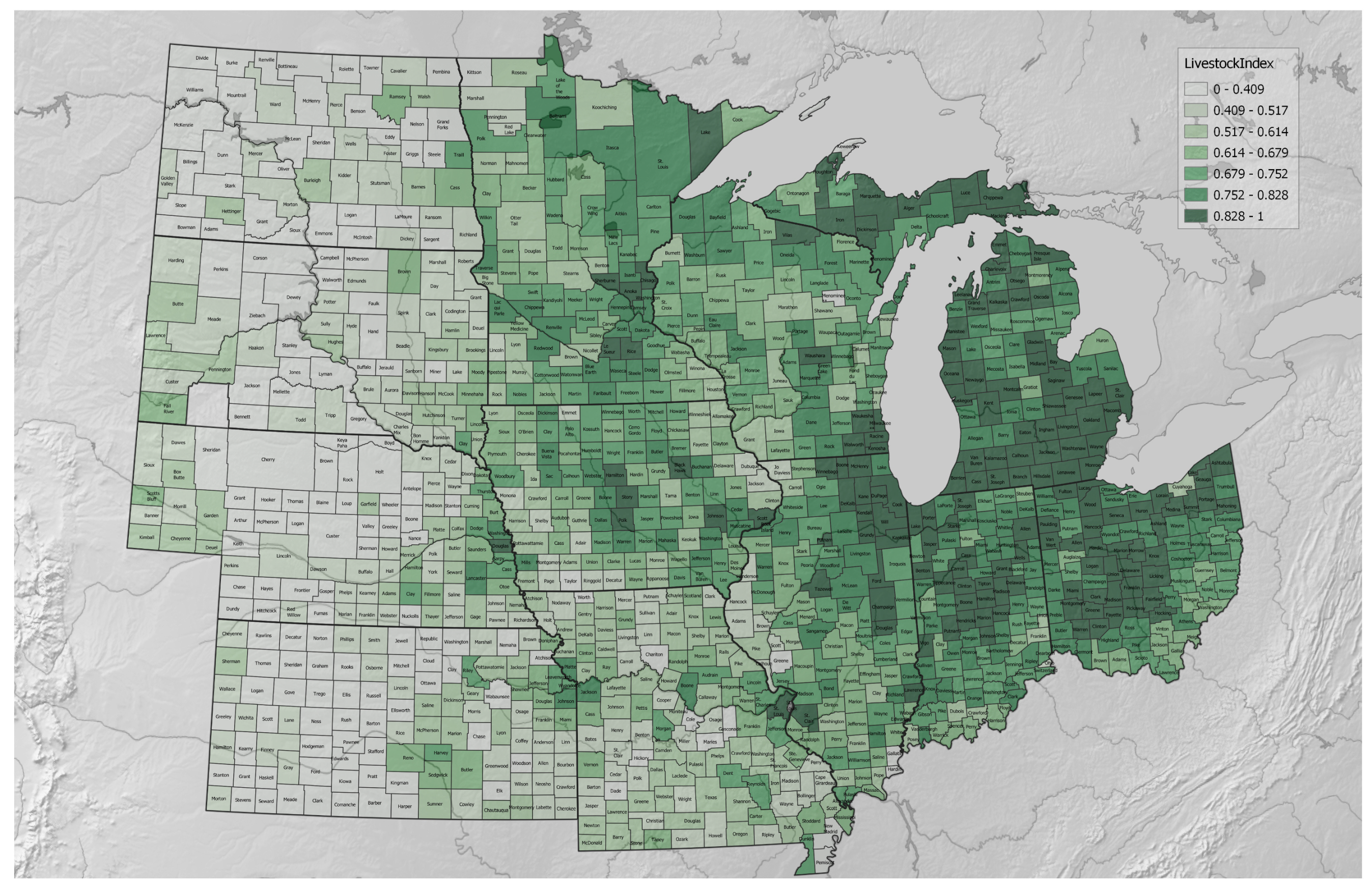
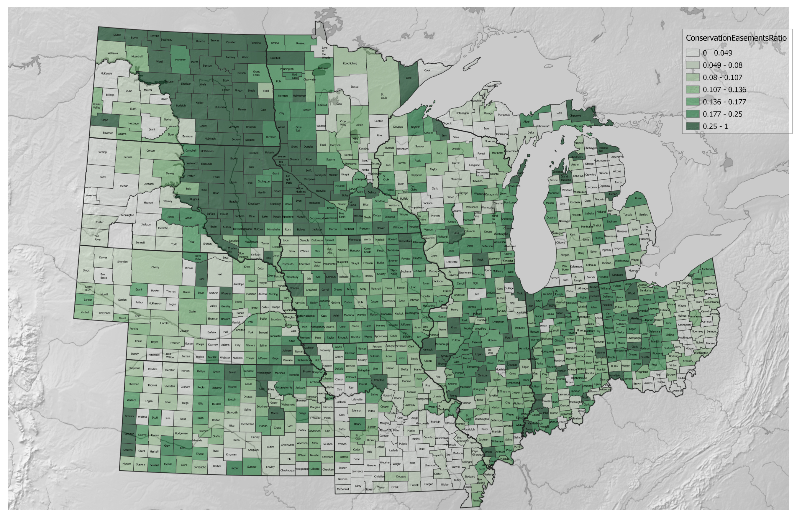
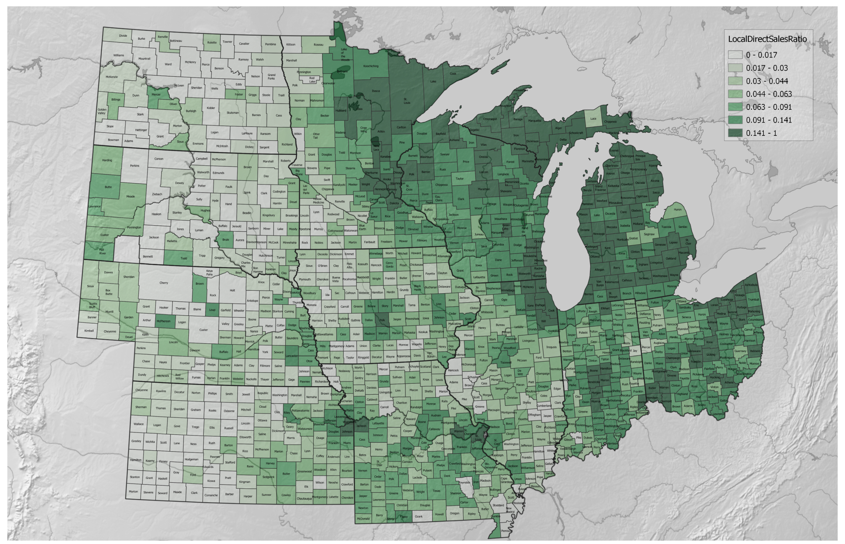
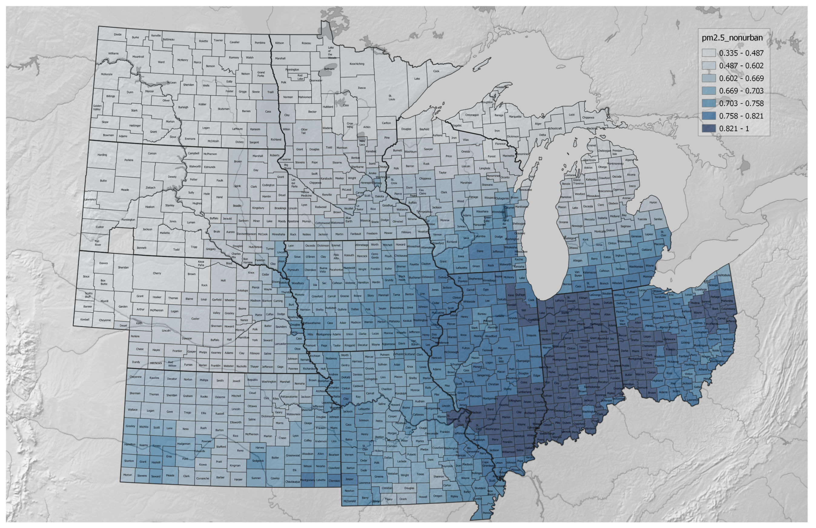
The variables that enter as terms in the numerator of the index ratio (those variables that are positively associated with regenerative agricultural lands) are mapped in Figure A1, Figure A2, Figure A3, Figure A4, Figure A5, Figure A6, Figure A7 and Figure A8. Those terms that are summed into the denominator of the index (those variables that are positively associated with conventional agricultural lands) are found in Figure A9, Figure A10, Figure A11, Figure A12 and Figure A13. We discuss aspects of these variables’ spatial distributions and contexts in the next two subsections on our index and clustering results. The relationships among the various variables considered here (as well as their relationships with the resulting agricultural index) are shown in Figure A15 through scatterplots and Spearman’s rank correlation coefficients. Among the latter, 93% of relationships have an absolute magnitude less than 0.6 out of a theoretical maximum of 1.0, although our methods do not assume independence; indeed, we expect and embrace a degree of dependence, spatial and otherwise, among variables. As seen below, our clustering approach obtains meaningful insights from spatially variable patterns of statistical dependence.

3.2. Agricultural Regenerative–Conventional Index

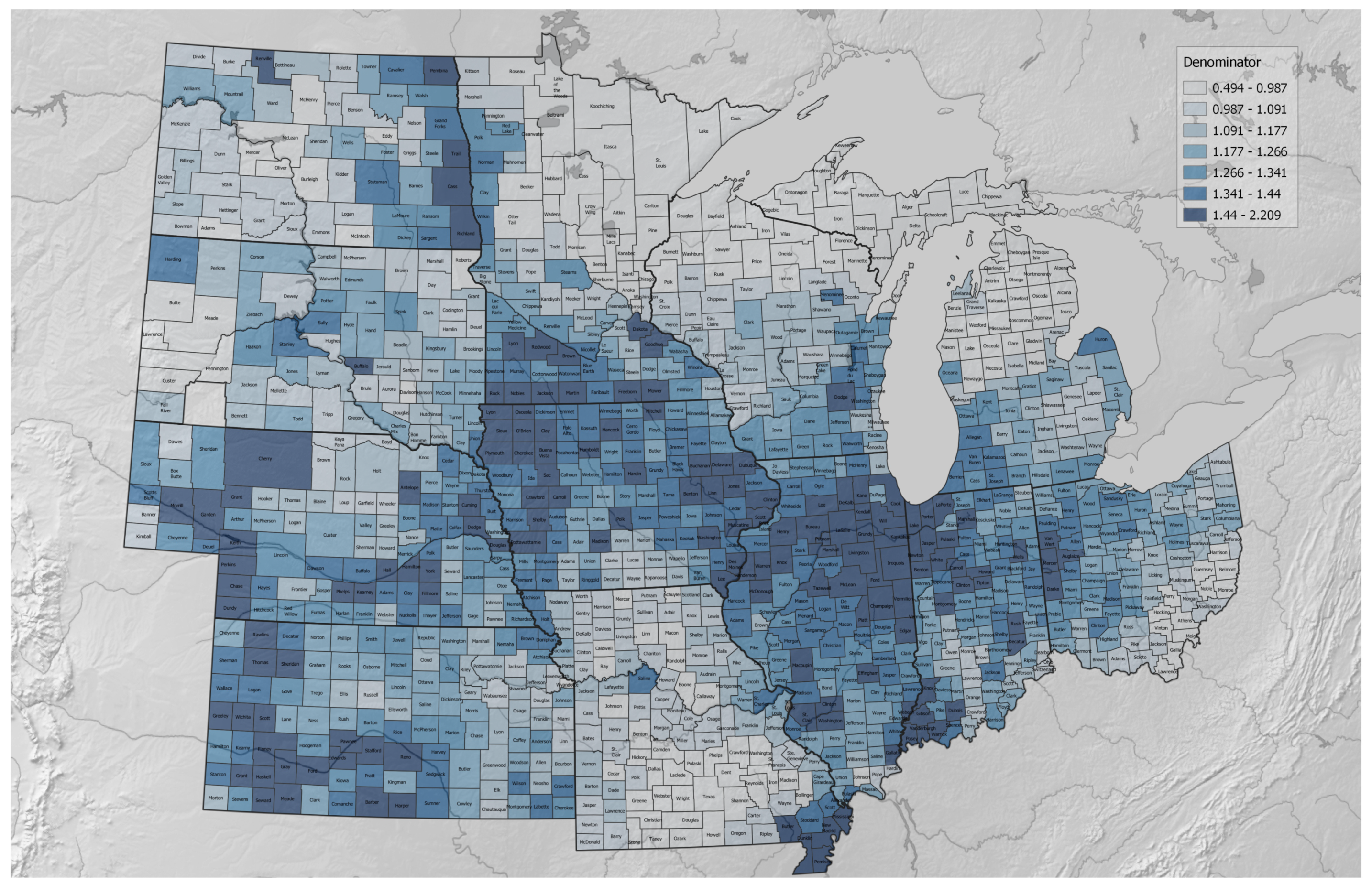
The resulting regenerative–conventional index was calculated and can be found mapped in Figure 1. Its component numerator and denominator are portrayed separately in Figure 2 and Figure 3, respectively. We highlight below some of the major features associated with each, as well as how they relate to each other and to the other variables that formed them. Those latter variables are mapped in Figure A1, Figure A2, Figure A3, Figure A4, Figure A5, Figure A6, Figure A7, Figure A8, Figure A9, Figure A10, Figure A11, Figure A12 and Figure A13. The complexity of these datasets is high, of course. What follows is a reading that tends to regionalize by foregrounding patterns at a particular scale, while other, less spatially contiguous or local-scale phenomena may remain yet unremarked upon.

3.2.1. Lands of Conventional Agriculture

The denominator, as mapped in Figure 2, aggregates variables we associated with conventional farming lands. There are significant swaths of territory over which many of the denominator variables align and yield high overall denominator values. One such belt includes northern Illinois, much of Iowa, and Minnesota south of the Minnesota River (with which there is a substantial, but by no means total, alignment with high-productivity corn-farming areas in those regions [74]), as well as the plains of Indiana and Ohio. In these regions, substantial contributions to the denominator are made by pesticides, farm average sizes, nonlocal food flows, and, in some areas, nonurban PM2.5 and agricultural methane emissions. The aforementioned variables are likewise often important to the substantial denominator values in the high plains of the west of Nebraska and Kansas. Minus the methane and PM2.5, the counties near the Red River between Minnesota and North Dakota have high denominator values from similar variables. Additional areas where the denominator is prominent occur in various clusters along the river valleys of the Missouri, the Platte, the Mississippi, and the Ohio. Regions with high values for the denominator appear to be associated with substantial numbers of denominator variables overlapping at high values. This is in seeming contrast with the numerator, where, as we see next, regions of relatively high numerator values appear to have more variety in the range of subsets of component variables that comprise those regions.

3.2.2. Lands of Regenerative Agriculture

By contrast, the numerator, in Figure 3, aggregates variables we associated with regenerative farming lands. Many of the counties near the Great Lakes have high numerators, although supportive reasons appear to differ slightly at multiple scales, from county to county and from state to state. In many of these areas, relatively high percentages of the land are forested. Silvopastoral practices are often prominent, perhaps with diverse livestock, a medium degree of intensive grazing, and both high local direct sales and high crop diversity. However, the numbers of farms are often lower than in some other areas where the numerator is also high.
One such region where there are more farms (which are still relatively small in size, on average) might be from southern Wisconsin up the Mississippi River valley to the Twin Cities in Minnesota, where diverse crops, relatively high local direct sales, the use of cover crops, and the use of no-till are important to a substantial regenerative numerator.
Much of Ohio has a high numerator, with a particularly prominent belt bisecting the state northeast to southwest roughly nearby the transition from the Alleghany plateaus to the lowland plains, with substantial parts of adjacent southern Indiana likewise having high numerator values, if more unevenly so. Livestock and crops are diverse through the belt in question, if not through all the states. Otherwise, the factors involved differ somewhat by place. Intensive grazing is high in the Appalachian plateaus and in relatively close proximities to the Ohio River at the southern edges of these states. Silvopasture is prominent in some of the more forested parts of Ohio. Cover crops are more important in northern Ohio and the southwestern hills and lowlands of Indiana. No-till is also used in the latter, although no-till practices are also prominent in much land near the Indiana–Ohio border.
Although not so in the eastern borderlands near the Red River, east–central North and South Dakota have many areas with high numerators. Conservation easements are common. Intensive grazing is high, if variable. No-till is common especially between the James and Missouri rivers. Crops are relatively diverse for the Great Plains states we considered.
Southern Iowa has relatively high numerator values, with which are associated various areas of intensive grazing, silvopasture, livestock diversity, conservation easements, no-till, crop diversity, and the use of cover crops. This area appears to have a mixture over space of different practices we associated with regenerative agricultural lands, a region that, for better or worse, would not have arisen as an entity able to be identified were it not for the construction of the index. By contrast, as we see below, a clustering approach finds southern Iowa to be split between several clusters.
A number of counties from the Missouri River in Missouri downstream along both banks of the Mississippi in Missouri and Illinois also have relatively high numerator values. Direct sales near metropolitan regions are high. Similarly, crop diversity is generally substantial but is especially so in proximity to the cities. Various counties practice higher levels of cover cropping, and silvopasture, more common in the Ozarks to the south, is still relatively common.
Areas in southeastern Nebraska and northeastern Kansas, south of the Platte River, commonly use no-till practices and have many counties with more conservation easements.
Lastly, north of the Platte in eastern Nebraska, cover crops, intensive grazing, a degree of crop diversity, and, if only in the eastern quarter of the state, no-till practices all contribute to a region with relatively high numerators.

3.2.3. Lands of the Regenerative–Conventional Agricultural Index

In some regions, the index is high because the denominator is low, and the numerator is high—as in lands of forests and lakes stretching from northern Minnesota over through to northern Michigan. Areas in the Dakotas both adjacent to the James River and of the high plains appear to have their own forms of such dynamics.
Likewise, there are areas where the index is low because the denominator is high, and the numerator is low. Notably, much of the areas with higher corn production in Minnesota, Iowa, and Illinois appear to have such dynamics, although there are areas of greater mixture of practices, as seen in a belt from western Illinois around Peoria across southern Iowa. Other areas of high denominator and low numerator include the Red River valley between Minnesota and North Dakota, as well as the western high plains of Kansas and Nebraska.
However, it is not always the case that a high denominator is associated with a low numerator, or a low denominator associated with a high numerator. Examining the index also suggests regions where neither numerator nor denominator is particularly high, but the ratio nonetheless tilts toward a higher index, such as in the Ozarks of Missouri or in several clusters of counties in the high plains of the Dakotas west of the Missouri River. Lastly, there are areas where both numerator and denominator are relatively high. There are regions such as those of central Ohio or southern Wisconsin, where the denominator is substantial, but the numerator is higher, yielding a relatively high index.

3.3. Agricultural Regenerative–Conventional Variable Clustering

The results above leverage the specific functional forms of the numerator, denominator, and resulting index ratio to infer and characterize regions of the midwestern landscape. Here, however, we present the results of characterizing the land through k-means cluster detection carried out on the same base variables before they were divided into numerator and denominator, summed, or divided. Results for nine clusters are shown in Figure 4 (maps of the clustering results where the number of clusters, k, ranges from 3 to 8 are available in Supplementary S1). Figure 5 and Figure 6 show how the various component variables are distributed across the counties within each of these clusters. All of the above, along with the spatial distributions of the input variables themselves shown in Figure A1, Figure A2, Figure A3, Figure A4, Figure A5, Figure A6, Figure A7, Figure A8, Figure A9, Figure A10, Figure A11, Figure A12 and Figure A13, are important for the synthetic results that follow.
Cluster 0/red runs intermittently along the Missouri River from the northwest of Missouri up into North Dakota, as well as much of eastern Nebraska and the Nebraska–Kansas border. Cluster 1/blue, similarly to cluster 0/red, and often adjacent to it, runs along several major rivers, including the Missouri up into North Dakota, the Platte in Nebraska, the southern half of Kansas centered on the Arkansas River, and, to a lesser extent, areas along the Mississippi. Cluster 1/blue has a significantly lower index value than 0/red; however, 1/blue has the second lowest of the nine clusters. It has a relatively high denominator and a very low numerator. It has relatively high levels of no-till, but not nearly as high as 0/red. Many of its farms have high crop diversities, with the third highest average. Although 1/blue has an unusually diverse range of farm sizes, it has the largest number of large farms, the highest nonlocal food flows, and substantial numbers of counties with either little local direct sales or livestock diversity.
These clusters likely bear comparison with cluster 5/yellow, which incorporates much rangeland and dominates the high plains north of the Platte and west of the Missouri in the Nebraska and the Dakotas, including the Sand Hills of Nebraska. Yellow has a regenerative index only slightly lower than 0/red, while its numerator and denominator are simultaneously much lower. It has the largest average farm size of the Midwest with the lowest livestock diversity and the highest rates of intensive grazing. Direct sales varied but were not the lowest; there was low pesticide use and, as in several of the lower index clusters, a bimodal distribution of crop diversity, with much low diversity and a lesser amount of higher diversity.
To the east of the Missouri River valley in the Dakotas, beyond the clusters mentioned above, lies cluster 7/pink. This region is centered around the James River running north–south and, thus, not as far east as the Red River or the Minnesota and Des Moines River basins (which form the heart of cluster 3/purple, discussed below). It has the third highest index of all clusters, with a higher numerator and a relatively low denominator. Low agricultural methane and nonurban PM2.5 contrast with the second largest average farm sizes, but other aspects of the denominator are relatively middling. In the numerator, however, the highest rates of conservation easements, high rates of no-till, above average crop diversity, and low (but significantly above the lowest) livestock diversity round out the reasonably high numerator. There is significant diversity from north to south in this region, however, with many of the counties nearer to the James River in eastern South Dakota up into North Dakota having among the highest regenerative numerators of the Great Plains.
A different situation obtains in cluster 3/purple, which, as mentioned, runs up the Red River south to the Minnesota River, and then encompasses much of southwestern Minnesota down into northern Iowa, with much of the relevant territory roughly centered around the Des Moines River basin. Substantial corn, soybean, and spring wheat production occurs in this cluster’s region. In the northern reaches, there are also substantial sugar beet harvests, which, interestingly, is also a feature of the isolated group of counties in this cluster located around Saginaw Bay off Lake Huron in Michigan. Cluster 3/purple has the lowest index of all the clusters, roughly tied with cluster 1/blue for the lowest numerator, while being roughly tied with 0/red for the second highest denominator. Its farms are of average size among the clusters, while smaller on average than the regions discussed above. Food flows over distance remain substantial, and pesticides are the most common among regions. Intensive grazing is the rarest, although livestock is relatively diverse. No-till is low, and crops are among the least diverse on a county-by-county level.
Beyond the southern borders of 3/purple in Iowa, stretching through eastern Iowa, most of Illinois, and the central till plains of Indiana stretching into the central lowland of Ohio, in regions known for corn and soybeans, among other production, we have cluster 8/gray. This region has a broad range of different numerators among counties, with its average near the median among counties. However, its denominator is mostly consistently the highest, and its average index is the third lowest overall. Pesticides and nonurban PM2.5 are high. Crop diversity is low; however, unlike cluster 3/purple, no-till is high. Livestock diversity is high, but intensive grazing is low.
Cluster 6/brown is found in a broad swath of counties surrounding much of cluster 8/gray, whether to the south near stretches of the Ohio River, to the west in northern Missouri and southern Iowa, or to the north in a swath from the Mississippi valley between Minnesota and Wisconsin through most of the southern halves of Wisconsin and Michigan. It is roughly tied for the second highest index value while having the second highest numerator and a median denominator. It has small farms, relatively low pesticides, high cover crop usage, diverse crops, diverse livestock, and relatively high presence of silvopastoral practices. Many of the areas with especially high numerator values along the Great Lakes lie within this region, as can be seen in Figure 3.
Cluster 2/green is split between southern Missouri and the Appalachian foothills of southwestern Ohio, with a few additional counties spread among the forests and lakes of cluster 4/orange (discussed below). Its index is slightly above the median among clusters, but it has relatively low numerators and denominators. While agricultural methane and nonurban PM2.5 are relatively high, pesticides are very low, farms are relatively small, and silvopastural practices, intensive grazing, and direct sales are relatively common.
Lastly, cluster 4/orange has the highest index value, having both the highest average numerator and the lowest average denominator. This cluster occurs in a broad range of the areas bordering the Great Lakes, encompassing Minnesota from the Twin Cities north and east, northern Wisconsin, the upper peninsula of Michigan, and northern Michigan. These areas, among forests, lakes, and sometimes urban areas, have the smallest farms, the most local shipments of products and direct sales, low pesticide use, low nonurban PM2.5, high use of cover crops, the most diverse crops, the most diverse livestock, and much silvopasture, while at the same time having the least use of no-till practices among regions.
Interested readers may find the dataset constructed and analyzed in this study, along with high-fidelity copies of the maps, at the following repository: https://doi.org/10.17605/OSF.IO/FYRZ8 (accessed on 16 March 2022).

4. Discussion

4.1. Co-producing Measurements and Mappings

In this study, we mapped regenerative and conventional agricultural lands of the US Midwest. We did so not by directly specifying a single empirical measurement to differentiate these lands, but by first coming to a group understanding of some processes and attributes that may lead to such landscapes, locating and calculating appropriate empirical measurements. Such co-production across epistemological domains—farmers, food analysts, and academics—represents a kind of consensus building process, both illuminating and limiting in its localized convergence. Cross-expertise accelerates identifying and operationalizing key variables, while also lending itself to a tendency toward choosing variables of a ‘common denominator’ across participants. Miller [66] describes a similar if more public collaborative research program, with which our research has some parallels in aims and outcomes, although there is less specific focus on the iterative co-generation of knowledge that determines the questions and variables chosen.
We then devised a single metric to synthesize these variables into an index describing agricultural lands as relatively regenerative, relatively conventional, and/or mixed in various ways. We also used clustering to determine which sorts of attributes and processes tended to be associated with each other, thereby regionalizing Midwest lands into a set of different agricultural regions associated with different blends of regenerative and conventional practices. We mapped those clustering regions, the index, the index’s component numerator (associated with regenerative lands) and denominator (associated with conventional ones), and all associated variables. We examined and characterized the resulting lands, interpreting them in light of other regional attributes, relations, and historical processes. Empirical conclusions may be found above. Readers are free to examine lands of interest to them, using the aforementioned resources to understand those lands either in deeper local context or in comparative analysis with other lands. Researchers may also compare our characterizations of the lands with other quantifications that they may be aware of or devise themselves.

4.2. Reading Multiple Mappings and Regionalizations

We proceed here to offer some additional observations about how the lands we identify using different approaches shed light on each other. Reading multiple mappings and associated regionalizations against each other yielded new insights. Seeming spatial continuities in the index, numerator, and/or denominator, even when examined with reference to their constituent variables, may nonetheless appear split into two or more clusters, either by a sharp line (see southern Iowa or the middle of the lower peninsula of Michigan) or by what appears likely to be a more ambiguous boundary (as in northern Missouri). Most clusters also suggest potential similarities in lands over discontinuities and long distances. At the same time, referring to the index and/or its numerator and denominator provides an important way of summarizing, comparing, and contrasting clusters, as seen in the differentiation of the Great Plains into lands that are regenerative, conventional, or simultaneously both.
Future research may include efforts to compare this article’s index or clustering with other such regionalizations and quantifications of land, as well as to better characterize the sensitivity of this index to changes in input variables, functional form, and geographical scope of counties included. We make several observations here suggesting how further inquiry in such directions may improve our empirical understanding about the lands we studied in particular, as well as contribute to the theory and method of multivariate analyses and syntheses of the land.
A series of efforts, first in the early 20th century [47,48,49], and then revisited in recent decades with shifting agricultural systems and the rise of digital computation [50,51], have attempted to characterize the geographies of agriculture in various areas of the world by dividing the land into homogeneous (but not necessarily contiguous) regions. Some methods are more quantitative than others. Past efforts have tended to consider similarities in agricultural products, farm sizes or revenues, interactions between farm and nonfarm sectors, and/or biophysical environmental contexts. Our regionalization approach considers some of those same variables, but not all, while we add consideration of a number of practices, connections, and consequences at farm, community, and regional scales. We are unaware of other research that combines and triangulates between regionalization- and index-based approaches. Past regionalizations differ in the number of regions they offer and, thus, the detail with which they subdivide the landscape, but none consider as many as nine regions within the Midwest as we do. Many studies end up finding regional divisions that largely reflect a set of primary products or activities and then name those regions accordingly. The boundaries of two such regions that appear in the maps of Baker [48] are ‘hay and dairying’ and the ‘corn belt’. There are some similarities between our cluster 6 and ‘hay and dairying’, on the one hand, and between the combination of our cluster 3 with cluster 8 and the ‘corn belt’, although this latter comparison is less convincing.
More recent regionalizations [50,51] are easier to compare and contrast with our results, perhaps because they are closer to our study in time and in their consideration of clustering methods, even if they differ somewhat in variables used. Our cluster 4 merged with cluster 6 bears some resemblance to the ‘Northern Crescent’ of the USDA Farm Resource Regions [51], although the latter lacks substantial land in cluster 6 that lies just beyond the southern edges of our cluster 8; all of that land lies within the USDA’s ‘Heartland’ region. Merging our clusters 5 and 7 yields a territory sharing substantial overlap with the USDA ‘Northern Great Plains’, but the latter lacks our nuances of counties along the Missouri River not being grouped with the rest of the neighboring region, instead having greater similarities to clusters 0 and 1 located further downriver and elsewhere in Kansas and Nebraska. Furthermore, in a rough sense, one could say our methods differentiated two clusters/regions (5 and 7) out of one USDA region (Northern Great Plains); however, those two clusters differ substantially in their engagement with regenerative agriculture, with cluster 7, to the east of the Missouri, having a much higher numerator than cluster 5, to the west of the Missouri. Lastly, our cluster 2 shares much in common, boundary-wise, with the parts of the USDA region ‘Eastern Uplands’ that lie within the 12 states we consider. The observation that our regionalization results have both similarities and differences with USDA Farm Resource Regions suggests that policies related to regenerative agriculture implemented with reference to the existing USDA Farm Resource Regions might be improved through the added consideration of the methods and results offered here.
With respect to future research into indices, greater consideration of variable weighting is warranted. Given that construction of the index required the combination of numbers with vastly different units, values, and distributions thereof, we chose to rescale each of the individual variables to range up to a unitless value of 1 by dividing all values of the variable distribution by the largest value found across all counties. Yet there is no reason the effective weight of each of these variables must be equal, although, in the absence of principles to the contrary, we left them such. Indeed, there are indices of great utility such as the Human Development Index that have likewise been designed with such weightings [75]. However, the field of multicriteria decision making and evaluation [76] has long considered various ways for individuals (or even conflicted groups) to thoughtfully integrate diverse information and values into quantifications. This is but one set of resources that could be brought to bear in further explorations of the functional form used in such quantifications of the land.
Salient aspects of regenerative and conventional agriculture must surely differ from region to region, as well as from interpreter to interpreter. There are implications for what an index could or should consist of. For example, Menominee County in Wisconsin has a very low regenerative index here (and only three entities reported as ‘farms’), but most of the land is a forest managed sustainably by Menominee peoples. Multiple salient aspects of that county’s practices are unlikely captured adequately by the present index, which highlights certain types of agriculture practiced more commonly by certain communities over others.
All indices are partial, but the partiality of the present index is necessarily a function of the concerns and experiences of the individuals constructing it. These concerns also have a regional and socioecological dimension to them. An index better suited to regenerative agriculture in the US Southwest, Haiti, or the Sichuan basin in China would likely involve choosing at least a somewhat different set of variables. The extent to which a single index with a single set of variables could reasonably exist that would capture something meaningful across substantial land and process diversity is a topic for future research. Under what ranges of diversity in regional practice and agroecologies might multiple indices be warranted?
Likewise, a variation on the manner in which the variable distributions are transformed before placing them into the index ratio (or other functional form, clustering analysis, etc.) might be to conduct more local normalizations. Perhaps instead of rescaling each variable by its maximum taken over the entirety of a macroregion of arbitrary extent (here, 12 states, although it could have, in principle, been six states or global), we might rescale the variables over more localized extents of a particular scale (e.g., of states or within a given radius). Such an approach might result in an index more attuned to the local variations of particular economic, climatic, or ecological regions. One could have each individual variable rescaled over its own characteristic differences according to the variation of the processes underlying that variable. Indeed, one can perceive differences in spatial scales of variation behind the visible spatial autocorrelations in the empirical distributions shown in the maps of the variables in the Appendix A. Such methodological developments in indices might enable them to respond to spatial process and heterogeneity.
While we position our work in a regenerative agriculture that extends production beyond the farm gate to community structures and processes, the variables included in our index are still aligned closely to on-farm practices and their impacts. A next iteration of our analysis could well converge upon a somewhat different emphasis that might change the set of variables in consequential ways. Would the results differ were we to add (then find/process data for) variables that looked not only at labor relations and property forms but also those able to offer a window on how locales were situated in the geographical and world-historical processes of globalizing late capitalism? How might our results differ if we were to have had variables that attempted to understand locales through ecological energetics or within biogeochemical cycles? How might gender, racialization, environmental justice, settler colonialism, and indigenous resurgence have been brought into the quantitative core of the index and affected the results?
Future such research might learn from Ludden et al. [45], who derived a Progressive Agriculture Index that encapsulates social, economic, and environmental factors, including farms with women and nonwhite principal operators, average farmworker wages, farm direct sales, farms with operators residing on site, and farms with community-supported agriculture and selling value-added products. It is useful to compare and contrast our results here with those offered by Ludden et al.’s index for 2007 and 2012 over the ‘lower 48’ states of the US. Ludden et al. found progressive conditions generally prevailing by county across the ‘Northern Crescent’ (one of the pre-existing USDA Farm Resource Regions [51] ranging from eastern Minnesota across Wisconsin, Michigan, and the northeast up to Maine), compared to other regions, roughly matching our overall index. The ‘Heartlands’ (from southern Minnesota and eastern sections of South Dakota and Nebraska, down through much of Missouri and across Illinois to eastern Ohio) ranked low in average county rank by the progressive index. The Northern Great Plains (including the Dakotas, northwest Minnesota, and northwest Nebraska) and the Prairie Gateway (including southern Nebraska and Kansas) ranked middling in the progressive index compared to other national regions. The Heartlands and Northern Great Plains supported low percentages of nonwhite principal operators, with some counties having none at all, even with nonwhite residents living in those counties. The Heartlands ranked last in regional measures of women-operated farms. The Prairie Gateway hosted the lowest percentages of farm operators living on site. All three discrepancies speak to historically conditioned barriers to farming entry: race, gender, and capital.
Specific counties in both regions, however, ranked high for Ludden et al.’s progressive index, and some ranked high for individual variables that contributed to their index. The Heartlands and Northern Great Plains, for example, hosted high average county ranks in wage as a percent of the federal minimum. Many of the counties in northeast Minnesota, northern Wisconsin, and northern Michigan ranked highly in both our regenerative–conventional agricultural index and in the Ludden et al. progressive agriculture index, keeping in mind the first was scaled across the Midwest, while the second was scaled nationally. On the other hand, the two indices also diverged. Our direct sales map (Figure A8) showed much more regional concentration of direct local sales for 2017 in the Great Lakes than Ludden et al.’s direct sales for 2012, which showed such sales widespread across the Midwest. This might be a matter of a change over time, but it may also be due to differences in variable definition. At the county level, Pierce County, North Dakota, ranked high in our agricultural index, but low by the overall progressive agriculture index. This suggests that regenerative practices can be focused at the level of on-farm practices—for instance, cover crops and low tillage—without changing the relations of production that still drive some of the most socioecologically destructive practices.
Similarly, Kuo and Peters [46] compiled an organic index against which they correlated a variety of socioeconomic variables, including the demographics the Ludden team pursued, as well as corporate farms, poverty, migration, a social capital index, and the Gini coefficient of income inequality, among other terms more directly related to human welfare. Considering the ecological and social origins of agricultural production, as well as the unique constellations of time and place counties represent, Kuo and Peters pursue a meso-level approach toward explaining organic production across US counties in 2007 and 2012. The resulting map of organic production is based on an explanatory factor analysis that looks much like the distribution for the regenerative variables in our index numerator for Minnesota and Wisconsin, but less so for Michigan, Indiana, and Ohio (Figure 3). Again, the time periods differ, as do the variables characterizing organic and regenerative production. Kuo and Peters found organics statistically associated with both demographic differences—e.g., more women operators—and modes of local economies, including the direct sales and CSA that our maps also suggest (Figure 3 and Figure A8). Their analysis, however, also found higher income, greater formal education, higher skilled professional occupations, and hillier land positively associated with organics intensity.

4.3. Revitalizing Regional Agricultural Geographies

At the same time, any of the above processes or relations, areas of vibrant scholarly research, need not be brought explicitly within the set of variables to be considered. Indeed, they are already reflected in all of our variables, in the regions derived from our clusters, and in our index. None of our variables exist in isolation from these important issues, but embody them. This is where our efforts to revitalize a regional geographic approach in the service of interpreting our quantitative results fall short in practice and must be an invitation to future research. Environmental historians, soil scientists, economic geographers, landscape ecologists, rural sociologists, and scholars in environmental studies, among many others, all know much about the agricultural lands we studied here. The challenge and opportunity is to rework that knowledge and revisit its various methods to interpret the variables, maps, and regions that we derived, yielding insightful regional geographies, ecologies, and environmental histories of the present.
We conclude by commenting on how our research approach relates to, is quite different from, and may be complemented by consideration of another class of approaches to understanding regenerative and conventional lands—those that first classify agricultural lands a priori as regenerative and/or conventional, only then inferring what characteristics define them. Whereas we proceeded from coming to consensus on processes that define regenerative lands, we might instead have attempted to identify those lands directly, and then determine which processes were empirically most closely associated with them. Under such circumstances, the differentiation of regenerative and conventional lands need not even be holistic or plural in its approach. It is conceivable that researchers might adopt a soil-centric approach to understanding regenerative agricultural lands and may devise a single variable to measure them, e.g., a measure of change in soil health over time, which is both theoretically justifiable and empirically available. Quantifications of how relevant aspects of soil health have been changing, available at a broad scope and sufficient resolution to be correlated with the locations of farmland being measured through the agricultural census (which would themselves need to be estimated, as they are not publicly available), have historically been difficult to obtain.
Advances in satellite technology and affordability, cloud computing, and remote sensing algorithms do make such research more plausible in the future [77,78,79,80]. With regenerative and/or conventional lands identified, a range of statistical and machine learning tools would likewise then become available, as the problem would be methodologically akin to inferring the socioecological ‘niche’ that a particular ‘species’ of agricultural land exists within. Future research might compare the portrayals of the land and its processes that would result from such inquiry, which proceeds from knowledge about land outcomes to processes, with the results we obtained here, which proceeded from knowledge about landscape processes to outcomes. The two approaches would complement each other.
The co-participatory means by which farming communities and researchers can arrive upon these measures together suggest that the policy implications of such work extend far beyond informing ‘decision makers’ acting top-down from state capitals, government agencies, or corporate boardrooms. Offered more analyses relevant to their aspirations and scales, rural communities may also serve themselves by choosing approaches specific to their regional objectives.

Supplementary Materials

The following supporting information can be downloaded at https://www.mdpi.com/article/10.3390/land11030437/s1: Supplement S1. Supplemental materials for ‘Mapping agricultural lands: from conventional to regenerative’. The supplement includes additional references [81,82] which are not included in the main text.

Author Contributions

Conceptualization, R.G.W., A.W., C.R.B., S.S., B.W., L.F.C. and L.B.; methodology, R.G.W., A.W., C.R.B., B.W., S.S., L.F.C. and L.B.; software, L.B., L.F.C. and B.W.; validation, C.R.B., B.W., L.F.C., R.G.W. and L.B.; formal analysis, C.R.B., B.W., L.F.C., R.G.W. and L.B.; investigation, C.R.B., B.W., L.F.C., R.G.W. and L.B.; resources, C.R.B., B.W., L.F.C., R.G.W. and L.B.; data curation, C.R.B., B.W., L.F.C., R.G.W. and L.B.; writing—original draft preparation, L.B., R.G.W. and L.F.C.; writing—review and editing, C.R.B., B.W., S.S., L.F.C., R.G.W. and L.B.; visualization, L.B.; supervision, R.G.W. and A.W.; project administration, R.G.W. and A.W.; funding acquisition, A.W., R.G.W., L.F.C. and L.B. All authors have read and agreed to the published version of the manuscript.

Funding

This research was funded by the Robert Wood Johnson Foundation’s Health and Climate Solutions program under the award “Regeneration Midwest: Scaling up climate and health solutions in agricultural communities across six US states”. Additional support came from the Canada Foundation for Innovation, WestGrid, Compute Canada, and the Canada Research Chairs Program.

Data Availability Statement

The dataset constructed and analyzed in this study, along with vector format originals of the maps, can be found at https://doi.org/10.17605/OSF.IO/FYRZ8 (accessed on 16 March 2022).

Acknowledgments

We thank Albina Gibadullina, Jim Thatcher, David O’Sullivan, and Nick Lally for useful suggestions regarding visualizations, Laura K. Paine for informative discussions in the conceptualization of the research and feedback on the manuscript, Pat Kerrigan and Kaare Melby for conceptual and logistical support, and Mariel Friberg for comments about the literature on the remote sensing of soil quality. We are grateful to the members of the Midwest Healthy Ag Research Advisory Committee for their assistance throughout the research.

Conflicts of Interest

The authors declare no conflict of interest. The funders had no role in the design of the study; in the collection, analyses, or interpretation of data; in the writing of the manuscript, or in the decision to publish the results.

Appendix A

This Appendix A contains visualizations of the key variables both forming the regenerative index and used in the clustering. The data are rendered large enough for individual counties to be distinguished while at the same time offering interested readers greater intuition behind both agriculture lands and the operation of the regenerative index.
The values are all divided by the largest value present for any of the counties over the 12 states of the US Midwest included here, as this transformation was applied to each of these variables as they were placed within the index formula. Variables from the numerator of the index’s ratio, those where a larger value offers the county a higher, more regenerative, index value, are portrayed using white to green color ramps (Figure A1, Figure A2, Figure A3, Figure A4, Figure A5, Figure A6, Figure A7 and Figure A8). Variables from the denominator of the index’s ratio, those where a larger value offers the county a lower, more conventional, index value, are portrayed using white to blue color ramps (Figure A9, Figure A10, Figure A11, Figure A12 and Figure A13). The map that follows (Figure A14) does not appear directly in the index but was used in calculating many of the aforementioned variables and is, thus, included here for reference. The data of Figure A14 are not rescaled by the maximum value, unlike all the other preceding maps in this Appendix A, nor does its color scheme follow the logics described above. Note that the methods and source data used to calculate all these variables are described above, in Section 2, with additional detail available in the Supplementary Materials. Lastly, Figure A15 offers a matrix scatterplot of the relationships among all pairs of a set of key variables, calculating Spearman’s rank correlation coefficients for each pairing, and offering a set of maps of each of the variables for convenience in interpreting the scatterplots. These maps differ from those of Figure A1, Figure A2, Figure A3, Figure A4, Figure A5, Figure A6, Figure A7, Figure A8, Figure A9, Figure A10, Figure A11, Figure A12 and Figure A13 not only in size but also in how the data are displayed; the color in the maps of Figure A15 is a continuous function of the variables at hand (thus, these are unclassified maps), whereas, in Figure A1, Figure A2, Figure A3, Figure A4, Figure A5, Figure A6, Figure A7, Figure A8, Figure A9, Figure A10, Figure A11, Figure A12 and Figure A13, the thematic variables are classified into seven bins of roughly equal numbers of counties. Each approach offers a different perspective on the underlying data.
Figure A1. Fraction of farms practicing intensive grazing, 2017. Values were all rescaled through dividing by the largest value present for any of the counties included here (0.422 in Thomas County, Nebraska), as this transformation was applied to the variable data as they were placed into the index expression. Methods for IntensiveGrazingRatio are described in the article main text and Supplementary Materials. USDA 2017 Census of Agriculture data [52] were used.
Land 11 00437 g0a1
Figure A2. Fraction of farms practicing silvopasture, 2017. Values were all rescaled through dividing by the largest value present for any of the counties included here (0.219 in Cook County, Minnesota), as this transformation was applied to the variable data as they were placed into the index expression. Methods for SilvopastureRatio are described in the article main text and Supplementary Materials. USDA 2017 Census of Agriculture data [52] were used.
Land 11 00437 g0a2
Figure A3. Livestock diversity index, by county, 2017. Values were all rescaled through dividing by the largest value present for any of the counties included here (1.977 in Crawford County, Michigan), as this transformation was applied to the variable data as they were placed into the index expression. Methods for LivestockDiversity are described in the article main text and Supplementary Materials. USDA 2017 Census of Agriculture data [52] were used.
Land 11 00437 g0a3
Figure A4. Fraction of farms with conservation easements, by county, 2017. Values were all rescaled through dividing by the largest value present for any of the counties included here (0.178 in Towner County, North Dakota), as this transformation was applied to the variable data as they were placed into the index expression. Methods for ConservationEasementsRatio are described in the article main text and Supplementary Materials. USDA 2017 Census of Agriculture data [52] were used.
Land 11 00437 g0a4
Figure A5. Fraction of farms planting cover crops, by county, 2017. Values were all rescaled through dividing by the largest value present for any of the counties included here (0.333 in Keweenaw County, Michigan), as this transformation was applied to the variable data as they were placed into the index expression. Methods for CoverCropsRatio are described in the article main text and Supplementary Materials. USDA 2017 Census of Agriculture data [52] were used.
Land 11 00437 g0a5
Figure A6. Fraction of farms practicing no-till, by county, 2017. Values were all rescaled through dividing by the largest value present for any of the counties included here (0.689 in Nuckolls County, Nebraska), as this transformation was applied to the variable data as they were placed into the index expression. Methods for NoTillRatio are described in the article main text and Supplementary Materials. USDA 2017 Census of Agriculture data [52] were used.
Land 11 00437 g0a6
Figure A7. Crop diversity index, by county, 2017. Values were all rescaled through dividing by the largest value present for any of the counties included here (1.343 in Cook County, Illinois), as this transformation was applied to the variable data as they were placed into the index expression. Methods for CropDiversity are described in the article main text and Supplementary Materials. USDA 2017 Census of Agriculture data [52] were used.
Land 11 00437 g0a7
Figure A8. Fraction of farms selling direct to consumers, by county, 2017. Values were all rescaled through dividing by the largest value present for any of the counties included here (0.667 in Keweenaw County, Michigan), as this transformation was applied to the variable data as they were placed into the index expression. Methods for LocalDirectSalesFarmsRatio are described in the article main text and Supplementary Materials. USDA 2017 Census of Agriculture data [52] were used.
Land 11 00437 g0a8
Figure A9. Average land area per farm, by county, 2017. Values were all rescaled through dividing by the largest value present for any of the counties included here (7736 acres per farm in Grant County, Nebraska), as this transformation was applied to the variable data as they were placed into the index expression. Methods for FarmSizeAvgAcres are described in the article main text and Supplementary Materials. USDA 2017 Census of Agriculture data [52] were used.
Land 11 00437 g0a9
Figure A10. Number of types of pesticides applied by the average farm, by county, 2017. Values were all rescaled through dividing by the largest value present for any of the counties included here (2.174 in Pemiscot County, Missouri), as this transformation was applied to the variable data as they were placed into the index expression. Methods for PesticideRatio are described in the article main text and Supplementary Materials. USDA 2017 Census of Agriculture data [52] were used.
Land 11 00437 g0a10
Figure A11. Average nonurban PM2.5, by county, 2016. Values were all rescaled through dividing by the largest value present for any of the counties included here (9.410 μg/m3 in Porter County, Indiana), as this transformation was applied to the variable data as they were placed into the index expression. Methods for PM2.5_nonurban are described in the article main text and Supplementary Materials. The map is based on data from WHO’s DIMAQ model estimates [61].
Land 11 00437 g0a11
Figure A12. Product of food exports by weight times distance traveled, only including domestic flows over 400 miles (644 km), 2012. Values were all rescaled through dividing by the largest value present for any of the counties included here (3.670 × 10⁶ kt-km from Richland County, North Dakota), as this transformation was applied to the variable data as they were placed into the index expression. Methods for Food_Flow_Over400mi_KTxKm are described in the article main text and Supplementary Materials. Data from [65] were used.
Land 11 00437 g0a12
Figure A13. Agricultural methane emissions per square kilometer, by county, 2012. Values were all rescaled through dividing by the largest value present for any of the counties included here (0.114 moles CH4 per second per square kilometer in St. Louis County, Missouri), as this transformation was applied to the variable data as they were placed into the index expression. Methods for CH4_per_km2_ag_area are described in the article main text and Supplementary Materials. Data from [67] were used.
Land 11 00437 g0a13
Figure A14. Number of farms per county, 2017. Methods for NumberOfFarms are described in the article main text and Supplementary Materials. USDA 2017 Census of Agriculture data [52] were used.
Land 11 00437 g0a14
Figure A15. Exploration of relationships among regenerative–conventional agricultural index variables. Scatter plots at the intersection of a given row and column corresponding to particular variables show the relations among those variables. Numbers are Spearman’s rank correlation coefficients. Maps along the diagonal show the spatial distribution of each variable.
Land 11 00437 g0a15

References

  1. Wender, M.J. Goodbye family farms and hello agribusiness: The story of how agricultural policy is destroying the family farm and the environment. Environ. Law J. 2011, 22, 141. [Google Scholar]
  2. Jones, B.A.; Grace, D.; Kock, R.; Alonso, S.; Rushton, J.; Said, M.Y.; McKeever, D.; Mutua, F.; Young, J.; McDermott, J.; et al. Zoonosis emergence linked to agricultural intensification and environmental change. Proc. Natl. Acad. Sci. USA 2013, 110, 8399–8404. [Google Scholar] [CrossRef] [PubMed] [Green Version]
  3. Chaves, L.F. The Dynamics of Latifundia Formation. PLoS ONE 2013, 8, e82863. [Google Scholar] [CrossRef] [PubMed] [Green Version]
  4. Howard, P.H. Concentration and Power in the Food System: Who Controls What We Eat? Bloomsbury Publishing: London, UK, 2021. [Google Scholar]
  5. Hill, J.; Goodkind, A.; Tessum, C.; Thakrar, S.; Tilman, D.; Polasky, S.; Smith, T.; Hunt, N.; Mullins, K.; Clark, M.; et al. Air-quality-related health damages of maize. Nat. Sustain. 2019, 2, 397–403. [Google Scholar] [CrossRef]
  6. General Mills. Regenerative Agriculture 2020. Available online: https://www.generalmills.com/en/Responsibility/Sustainability/Regenerative-agriculture (accessed on 14 February 2022).
  7. Wezel, A.; Casagrande, M.; Celette, F.; Vian, J.-F.; Ferrer, A.; Peigné, J. Agroecological practices for sustainable agriculture—A review. Agron. Sustain. Dev. 2014, 34, 1–20. [Google Scholar] [CrossRef] [Green Version]
  8. Altieri, M.A. Agroecology: The Science of Sustainable Agriculture; CRC Press: Boca Raton, FL, USA, 2018. [Google Scholar]
  9. Altieri, M.A.; Nicholls, C.I.; Montalba, R. Technological approaches to sustainable agriculture at a crossroads: An agroecological perspective. Sustainability 2017, 9, 349. [Google Scholar] [CrossRef] [Green Version]
  10. Rhodes, C.J. The imperative for regenerative agriculture. Sci. Prog. 2017, 100, 80–129. [Google Scholar] [CrossRef]
  11. Urrutia, A.L.; González-Gónzalez, C.; Van Cauwelaert, E.M.; Rosell, J.A.; García Barrios, L.; Benítez, M. Landscape heterogeneity of peasant-managed agricultural matrices. Agric. Ecosyst. Environ. 2020, 292, 106797. [Google Scholar] [CrossRef]
  12. Gebru, H. A review on the comparative advantages of intercropping to mono-cropping system. J. Biol. Agric. Healthc. 2015, 5, 1–13. [Google Scholar]
  13. Kantola, I.; Masters, M.; DeLucia, E. Soil particulate organic matter increases under perennial bioenergy crop agriculture. Soil Biol. Biochem. 2017, 113, 184–191. [Google Scholar] [CrossRef]
  14. Kaye, J.P.; Quemada, M. Using cover crops to mitigate and adapt to climate change—A review. Agron. Sustain. Dev. 2017, 37, 4. [Google Scholar] [CrossRef]
  15. Busari, M.A.; Kukal, S.S.; Kaur, A.; Bhatt, R.; Dulazi, A.A. Conservation tillage impacts on soil, crop and the environment. Int. Soil Water Conserv. Res. 2015, 3, 119–129. [Google Scholar] [CrossRef] [Green Version]
  16. Chen, W.; Huang, D.; Liu, N.; Zhang, Y.; Badgery, W.; Wang, X.; Shen, Y. Improved grazing management may increase soil carbon sequestration in temperate steppe. Sci. Rep. 2015, 5, 10892. [Google Scholar] [CrossRef] [PubMed] [Green Version]
  17. Sulc, R.M.; Tracy, B.F. Integrated Crop–Livestock Systems in the U.S. Corn Belt. Agron. J. 2007, 99, 335–345. [Google Scholar] [CrossRef] [Green Version]
  18. Griffon, D.; Hernandez, M.-J. Some theoretical notes on agrobiodiversity: Spatial heterogeneity and population interactions. Agroecol. Sustain. Food Syst. 2020, 44, 795–823. [Google Scholar] [CrossRef]
  19. Levins, R.; Wilson, M. Ecological Theory and Pest-Management. Annu. Rev. Entomol. 1980, 25, 287–308. [Google Scholar] [CrossRef]
  20. Altieri, M.A.; Nicholls, C.I. Ecologically based pest management: A key pathway to achieving agroecosystem health. In Managing for Healthy Ecosystems; CRC Press: Boca Raton, FL, USA, 2002; pp. 999–1010. [Google Scholar]
  21. Borin, M.; Passoni, M.; Thiene, M.; Tempesta, T. Multiple functions of buffer strips in farming areas. Eur. J. Agron. 2010, 32, 103–111. [Google Scholar] [CrossRef]
  22. Scherr, S.J.; Shames, S.; Friedman, R. From climate-smart agriculture to climate-smart landscapes. Agric. Food Secur. 2012, 1, 12. [Google Scholar] [CrossRef] [Green Version]
  23. Cole, L.J.; Brocklehurst, S.; Robertson, D.; Harrison, W.; McCracken, D.I. Riparian buffer strips: Their role in the conservation of insect pollinators in intensive grassland systems. Agric. Ecosyst. Environ. 2015, 211, 207–220. [Google Scholar] [CrossRef]
  24. Cook, S.M.; Khan, Z.R.; Pickett, J.A. The Use of Push-Pull Strategies in Integrated Pest Management. Annu. Rev. Entomol. 2007, 52, 375–400. [Google Scholar] [CrossRef] [PubMed] [Green Version]
  25. Rodale Institute. Regenerative Organic Agriculture and Climate Change: A Down-to-Earth Solution to Global Warming. 2015. Available online: https://rodaleinstitute.org/wp-content/uploads/rodale-white-paper.pdf (accessed on 14 February 2022).
  26. Rui, Y.; Jackson, R.D.; Cotrufo, M.F.; Sanford, G.R.; Spiesman, B.J.; Deiss, L.; Culman, S.W.; Liang, C.; Ruark, M.D. Persistent soil carbon enhanced in Mollisols by well-managed grasslands but not annual grain or dairy forage cropping systems. Proc. Natl. Acad. Sci. USA 2022, 119, e2118931119. [Google Scholar] [CrossRef] [PubMed]
  27. Toensmeier, E. The Carbon Farming Solution; A global toolkit of perennial crops and regenerative agriculture practices for climate change mitigation and food security; Chelsea Green Publishing: Hartford, VT, USA, 2016. [Google Scholar]
  28. Montgomery, D.R.; Biklé, A.; Archuleta, R.; Brown, P.; Jordan, J. Soil health and nutrient density: Preliminary comparison of regenerative and conventional farming. PeerJ 2022, 10, e12848. [Google Scholar] [CrossRef] [PubMed]
  29. Perfecto, I.; Vandermeer, J.; Wright, A. Nature’s Matrix: Linking Agriculture, Biodiversity Conservation and Food Sovereignty; Routledge: London, UK, 2019. [Google Scholar]
  30. Giraldo, O.F. Political Ecology of Agriculture; Springer: Cham, Switzerland, 2019; 150p. [Google Scholar]
  31. Duncan, J.; Carolan, M.S.; Wiskerke, J.S. Routledge Handbook of Sustainable and Regenerative Food Systems; Routledge: London, UK, 2021. [Google Scholar]
  32. Longo, P. Food justice and sustainability: A new revolution. Agric. Agric. Sci. Procedia 2016, 8, 31–36. [Google Scholar] [CrossRef] [Green Version]
  33. Penniman, L. Farming While Black: Soul Fire Farm’s Practical Guide to Liberation on the Land; Chelsea Green Publishing: Hartford, VT, USA, 2018. [Google Scholar]
  34. Arias, P.F.; Jonas, T.; Munksgaard, K. Farming Democracy: Radically Transforming the Food System from the Ground Up; Australian Food Sovereignty Alliance: Melbourne, VIC, Australia, 2019. [Google Scholar]
  35. Slocum, R.; Cadieux, K.V. Notes on the practice of food justice in the US: Understanding and confronting trauma and inequity. J. Political Ecol. 2015, 22, 27. [Google Scholar]
  36. Rotz, S.; Fraser, E.D. Resilience and the industrial food system: Analyzing the impacts of agricultural industrialization on food system vulnerability. J. Environ. Stud. Sci. 2015, 5, 459–473. [Google Scholar] [CrossRef]
  37. Frison, E.A.; IPES-Food. From Uniformity to Diversity: A Paradigm Shift from Industrial Agriculture to Diversified Agroecological Systems; IPES: Louvain-la-Neuve, Belgium, 2016; 96p. [Google Scholar]
  38. Burchi, F.; Fanzo, J.; Frison, E. The role of food and nutrition system approaches in tackling hidden hunger. Int. J. Environ. Res. Public Health 2011, 8, 358–373. [Google Scholar] [CrossRef] [PubMed]
  39. Zenk, S.N.; Schulz, A.J.; Israel, B.A.; James, S.A.; Bao, S.; Wilson, M.L. Fruit and vegetable access differs by community racial composition and socioeconomic position in Detroit, Michigan. Ethn. Dis. 2006, 16, 275–280. [Google Scholar] [PubMed]
  40. Harden, N.M.; Ashwood, L.L.; Bland, W.L.; Bell, M.M. For the public good: Weaving a multifunctional landscape in the Corn Belt. Agric. Hum. Values 2013, 30, 525–537. [Google Scholar] [CrossRef]
  41. Low, S.A.; Adalja, A.; Beaulieu, E.; Key, N.; Martinez, S.; Melton, A.; Perez, A.; Ralston, K.; Stewart, H.; Suttles, S.; et al. Trends in US Local and Regional Food Systems: A Report to Congress; Cornell SC Johnson College of Business: Ithaca, NY, USA, 2015. [Google Scholar]
  42. Rotz, S.; Fraser, E.D.; Martin, R.C. Situating tenure, capital and finance in farmland relations: Implications for stewardship and agroecological health in Ontario, Canada. J. Peasant Stud. 2019, 46, 142–164. [Google Scholar] [CrossRef]
  43. Chappell, M.J. Beginning to End Hunger: Food and the Environment in Belo Horizonte, Brazil, and Beyond; University of California Press: Berkeley, CA, USA, 2018. [Google Scholar]
  44. Fenster, T.L.; LaCanne, C.E.; Pecenka, J.R.; Schmid, R.B.; Bredeson, M.M.; Busenitz, K.M.; Michels, A.M.; Welch, K.D.; Lundgren, J.G. Defining and validating regenerative farm systems using a composite of ranked agricultural practices. F1000Research 2021, 10, 115. [Google Scholar] [CrossRef]
  45. Ludden, M.T.; Welsh, R.; Weissman, E.; Hilchey, D.; Gillespie, G.W.; Guptill, A. The Progressive Agriculture Index: Assessing the Advancement of Agri-food Systems. J. Agric. Food Syst. Community Dev. 2018, 8, 159–185. [Google Scholar] [CrossRef]
  46. Kuo, H.-J.; Peters, D.J. The socioeconomic geography of organic agriculture in the United States. Agroecol. Sustain. Food Syst. 2017, 41, 1162–1184. [Google Scholar] [CrossRef] [Green Version]
  47. Jonasson, O. Agricultural Regions of Europe. Econ. Geogr. 1925, 1, 277–314. [Google Scholar] [CrossRef]
  48. Baker, O.E. Agricultural Regions of North America. Part I. The Basis of Classification. Econ. Geogr. 1926, 2, 459–493. [Google Scholar] [CrossRef]
  49. Whittlesey, D. Major Agricultural Regions of the Earth. Ann. Assoc. Am. Geogr. 1936, 26, 199–240. [Google Scholar] [CrossRef]
  50. Sommer, J.E. Diversity in US Agriculture: A New Delineation by Farming Characteristics; US Department of Agriculture, Economic Research Service: Washington, DC, USA, 1991.
  51. U.S. Department of Agriculture, Economic Research Service. Farm Resource Regions; AIB-760; US Department of Agriculture, Economic Research Service: Washington, DC, USA, 2000. Available online: www.ers.usda.gov/publications/aib760/ (accessed on 11 March 2022).
  52. United States Department of Agriculture, National Agricultural Statistics Service. 2017 Census of Agriculture Washington DC: United States Department of Agriculture. 2019. Available online: https://www.nass.usda.gov/Publications/AgCensus/2017/index.php (accessed on 14 February 2022).
  53. Sulc, R.M.; Franzluebbers, A.J. Exploring integrated crop–livestock systems in different ecoregions of the United States. Eur. J. Agron. 2014, 57, 21–30. [Google Scholar] [CrossRef]
  54. Scherr, S.J.; McNeely, J.A. Biodiversity conservation and agricultural sustainability: Towards a new paradigm of ‘ecoagriculture’ landscapes. Philos. Trans. R. Soc. B Biol. Sci. 2008, 363, 477–494. [Google Scholar] [CrossRef] [PubMed] [Green Version]
  55. Qiu, J.; Wardropper, C.B.; Rissman, A.R.; Turner, M.G. Spatial fit between water quality policies and hydrologic ecosystem services in an urbanizing agricultural landscape. Landsc. Ecol. 2017, 32, 59–75. [Google Scholar] [CrossRef]
  56. Sanderson, M.A.; Archer, D.; Hendrickson, J.; Kronberg, S.; Liebig, M.; Nichols, K.; Schmer, M.; Tanaka, D.; Aguilar, J. Diversification and ecosystem services for conservation agriculture: Outcomes from pastures and integrated crop–livestock systems. Renew. Agric. Food Syst. 2013, 28, 129–144. [Google Scholar] [CrossRef] [Green Version]
  57. Willis, G.H.; McDowell, L.L. Pesticides in agricultural runoff and their effects on downstream water quality. Environ. Toxicol. Chem. 1982, 1, 267–279. [Google Scholar] [CrossRef]
  58. Rasmussen, J.J.; Wiberg-Larsen, P.; Baattrup-Pedersen, A.; Monberg, R.J.; Kronvang, B. Impacts of pesticides and natural stressors on leaf litter decomposition in agricultural streams. Sci. Total Environ. 2012, 416, 148–155. [Google Scholar] [CrossRef] [Green Version]
  59. Dwivedi, A.K. Researches in water pollution: A review. Int. Res. J. Nat. Appl. Sci. 2017, 4, 118–142. [Google Scholar]
  60. Chaudhry, F.N.; Malik, M. Factors affecting water pollution: A review. J. Ecosyst. Ecography 2017, 7, 1–3. [Google Scholar]
  61. Shaddick, G.; Thomas, M.; Green, A.; Brauer, M.; Van Donkelaar, A.; Burnett, R.; Chang, H.H.; Cohen, A.; Van Dingenen, R.; Dora, C.; et al. Data integration model for air quality: A hierarchical approach to the global estimation of exposures to ambient air pollution. J. R. Stat. Soc. Ser. C (Appl. Stat.) 2017, 67, 231–253. [Google Scholar] [CrossRef]
  62. Dewitz, J. National Land Cover Database (NLCD) 2016 Products. In U.S. Geological Survey Data Release; editor. ver. 2.0, July 2020 ed2019; U.S. Geological Survey: Sioux Falls, SD, USA, 2019. [Google Scholar] [CrossRef]
  63. Domingo, N.G.G.; Balasubramanian, S.; Thakrar, S.K.; Clark, M.A.; Adams, P.J.; Marshall, J.D.; Muller, N.Z.; Pandis, S.N.; Polasky, S.; Robinson, A.L.; et al. Air quality–related health damages of food. Proc. Natl. Acad. Sci. USA 2021, 118, e2013637118. [Google Scholar] [CrossRef]
  64. Food, Conservation, and Energy Act of 2008, Pub. L. 110-246, 122 Stat. 1929. Available online: https://www.govinfo.gov/content/pkg/PLAW-110publ246/html/PLAW-110publ246.htm (accessed on 5 March 2022).
  65. Lin, X.; Ruess, P.J.; Marston, L.; Konar, M. Food flows between counties in the United States. Environ. Res. Lett. 2019, 14, 084011. [Google Scholar] [CrossRef]
  66. Miller, M. Identifying Critical Thresholds for Resilient Regional Food Flows: A Case Study from the U.S. Upper Midwest. Front. Sustain. Food Syst. 2021, 5, 371. [Google Scholar] [CrossRef]
  67. Maasakkers, J.D.; Jacob, D.J.; Sulprizio, M.P.; Turner, A.; Weitz, M.; Wirth, T.; Hight, C.; Defigueiredo, M.; Desai, M.; Schmeltz, R.; et al. Gridded National Inventory of U.S. Methane Emissions. Environ. Sci. Technol. 2016, 50, 13123–13133. [Google Scholar] [CrossRef] [PubMed]
  68. Hristov, A.N.; Harper, M.; Meinen, R.; Day, R.; Lopes, J.; Ott, T.; Venkatesh, A.; Randles, C.A. Discrepancies and Uncertainties in Bottom-up Gridded Inventories of Livestock Methane Emissions for the Contiguous United States. Environ. Sci. Technol. 2017, 51, 13668–13677. [Google Scholar] [CrossRef] [PubMed]
  69. Jain, A.K. Data clustering: 50 years beyond K-means. Pattern Recognit. Lett. 2010, 31, 651–666. [Google Scholar] [CrossRef]
  70. Kazakov, E. Attribute Based Clustering 2019. Available online: https://github.com/eduard-kazakov/attributeBasedClustering (accessed on 5 March 2022).
  71. Virtanen, P.; Gommers, R.; Oliphant, T.E.; Haberland, M.; Reddy, T.; Cournapeau, D.; Burovski, E.; Peterson, P.; Weckesser, W.; Bright, J.; et al. SciPy 1.0: Fundamental algorithms for scientific computing in Python. Nat. Methods 2020, 17, 261–272. [Google Scholar] [CrossRef] [PubMed] [Green Version]
  72. Bunge, W. Locations are not unique. Ann. Assoc. Am. Geogr. 1966, 56, 375–376. [Google Scholar] [CrossRef]
  73. Hartshorne, R. Perspective on the Nature of Geography; Association of American Geographers: Philadelphia, PA, USA, 1959; 201p. [Google Scholar]
  74. United States Department of Agriculture, National Agricultural Statistics Service. Corn: Production Acreage by County—2019; United States Department of Agriculture National Agricultural Statistics Service: Washington, DC, USA, 2020. Available online: https://www.nass.usda.gov/Charts_and_Maps/Crops_County/cr-pr.php (accessed on 5 March 2022).
  75. Anand, S.; Sen, A. Human Development Index: Methodology and Measurement; Human Development Report Office: New York, NY, USA, 1994; 19p. [Google Scholar]
  76. Malczewski, J.; Rinner, C. Multicriteria Decision Analysis in Geographic Information Science; Springer: New York, NY, USA, 2015; 331p. [Google Scholar]
  77. Lobell, D.B. Remote Sensing of Soil Degradation: Introduction. J. Environ. Qual. 2010, 39, 1–4. [Google Scholar] [CrossRef] [PubMed]
  78. Cécillon, L.; Barthès, B.G.; Gomez, C.; Ertlen, D.; Genot, V.; Hedde, M.; Stevens, A.; Brun, J.J. Assessment and monitoring of soil quality using near-infrared reflectance spectroscopy (NIRS). Eur. J. Soil Sci. 2009, 60, 770–784. [Google Scholar] [CrossRef] [Green Version]
  79. Paz-Kagan, T.; Zaady, E.; Salbach, C.; Schmidt, A.; Lausch, A.; Zacharias, S.; Notesco, G.; Ben-Dor, E.; Karnieli, A. Mapping the Spectral Soil Quality Index (SSQI) Using Airborne Imaging Spectroscopy. Remote Sens. 2015, 7, 15748–15781. [Google Scholar] [CrossRef] [Green Version]
  80. De Paul Obade, V.; Lal, R. Assessing land cover and soil quality by remote sensing and geographical information systems (GIS). Catena 2013, 104, 77–92. [Google Scholar] [CrossRef]
  81. Roth, J. County Distance Database: National Bureau of Economic Research. 2014. Available online: https://data.nber.org/data/county-distance-database.html (accessed on 15 February 2022).
  82. United States Census Bureau. 2017 TIGER/Line Shapefiles. Available online: https://www.census.gov/geographies/mapping-files/time-series/geo/tiger-line-file.html (accessed on 15 February 2022).
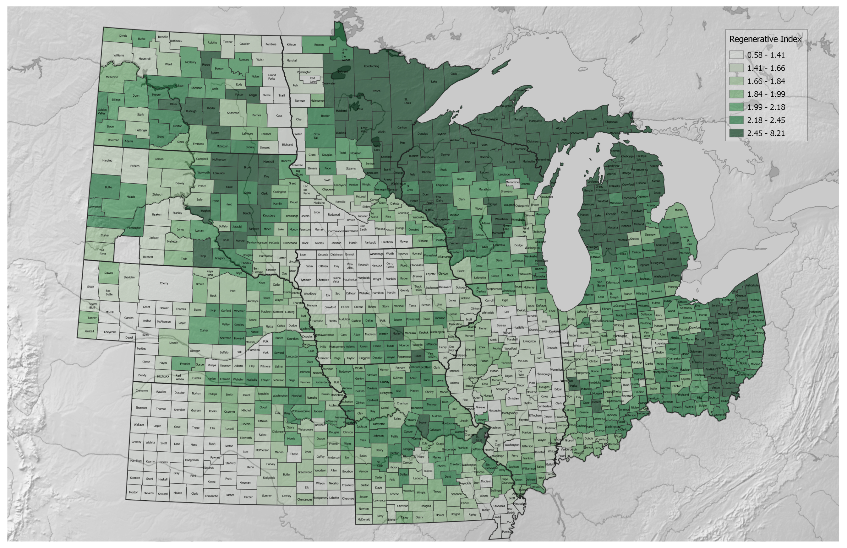
Figure 1. Regenerative–conventional agricultural index—a ratio between a ‘numerator’ composed of variables associated with regenerative agricultural lands and a ‘denominator’ composed of variables associated with conventional agricultural lands. Lower index values, thus, are associated with counties whose agricultural lands are more conventional. Higher index values are associated with counties whose agricultural lands are more regenerative.
Land 11 00437 g001
Figure 2. Regenerative–conventional agricultural index ratio denominator—the sum of variables we associated positively with conventional agricultural lands.
Land 11 00437 g002
Figure 3. Regenerative–conventional agricultural index ratio numerator—the sum of variables we associated positively with regenerative agricultural lands.
Land 11 00437 g003
Figure 4. Counties whose regenerative–conventional variable values are close to one another, as found using k-means clustering for k = 9.
Land 11 00437 g004
Figure 5. Histograms of index denominator variables broken out by county cluster membership. Each cluster’s counties have a row; each variable has a column. Although clusters are not calculated on the overall index, nor on the numerator or denominator, those three derived variables are presented here for reference in the leftmost three columns. Indeed, cluster rows are sorted by their overall regenerative index. A vertical black line indicates the mean value for the variables in its cluster. Note that, for efficient use of space on the visualization, the 7% highest and 7% lowest values for a given variable (regardless of which cluster they may be contained in) are not shown at their correct x-values; they are instead stacked in the histogram in the bins where the 7th and 93rd percentiles would be displayed, respectively. Vertical lines for mean values, however, are not constrained in this way but appear at their proper values, which on occasion leads to some of them seeming to appear outside of the distribution.
Land 11 00437 g005
Figure 6. Histograms of index numerator variables broken out by county cluster membership. Each cluster’s counties have a row; each variable has a column. Although clusters are not calculated on the overall index, nor on the numerator or denominator, those three derived variables are presented here for reference in the rightmost three columns. Indeed, cluster rows are sorted by their overall regenerative index. A vertical black line indicates the mean value for the variables in its cluster. Note that, for efficient use of space on the visualization, the 7% highest and 7% lowest values for a given variable (regardless of which cluster they may be contained in) are not shown at their correct x-values; they are instead stacked in the histogram in the bins where the 7th and 93rd percentiles would be displayed, respectively. Vertical lines for mean values, however, are not constrained in this way but appear at their proper values, which on occasion leads to some of them seeming to appear outside of the distribution.
Land 11 00437 g006
Publisher’s Note: MDPI stays neutral with regard to jurisdictional claims in published maps and institutional affiliations.