
Analysis of Land Use Change and the Role of Policy Dimensions in Ecologically Complex Areas: A Case Study in Chongqing

Abstract
:1. Introduction
2. Data and Methods
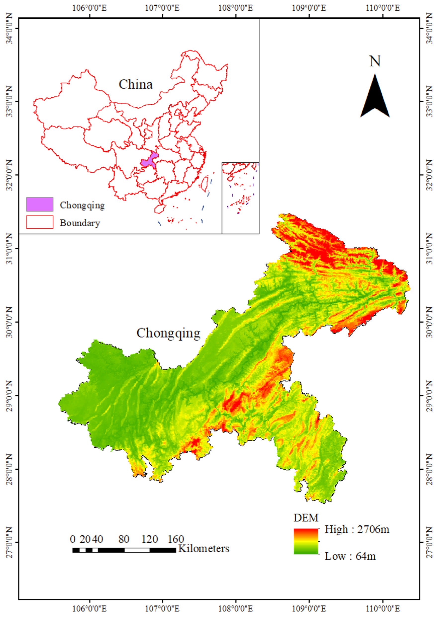
2.1. Study Area
2.2. Data Sources
2.3. Method
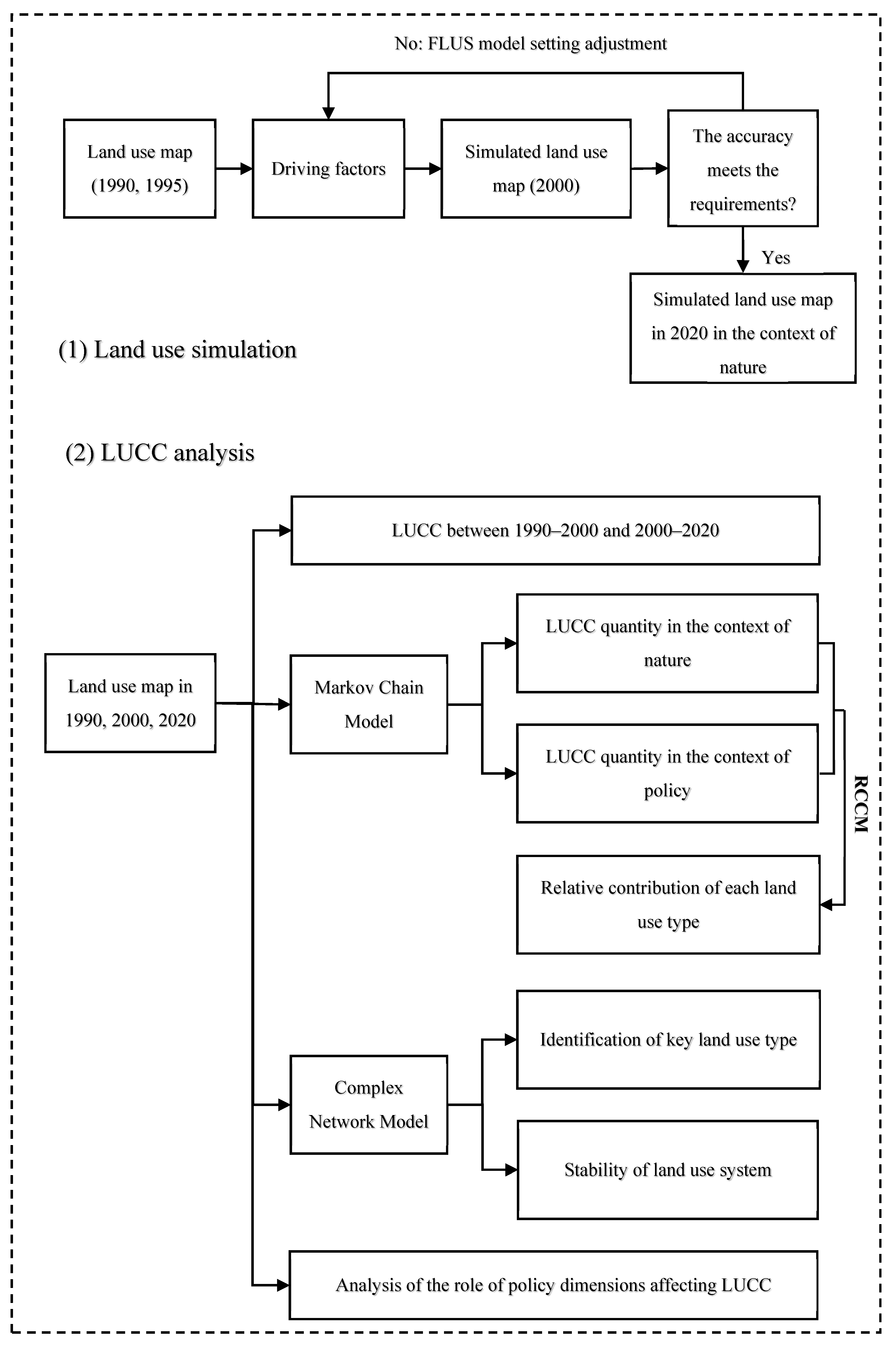
2.3.1. Research Framework
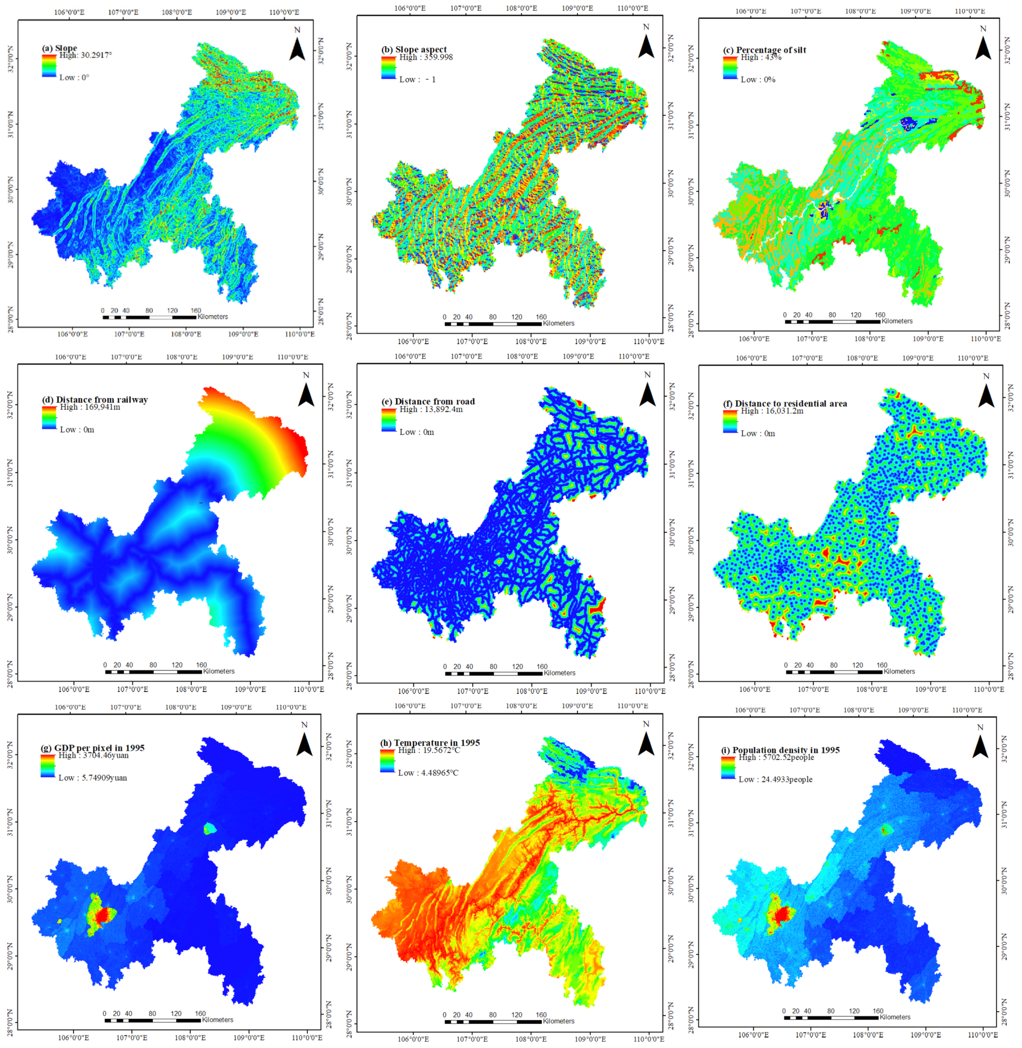
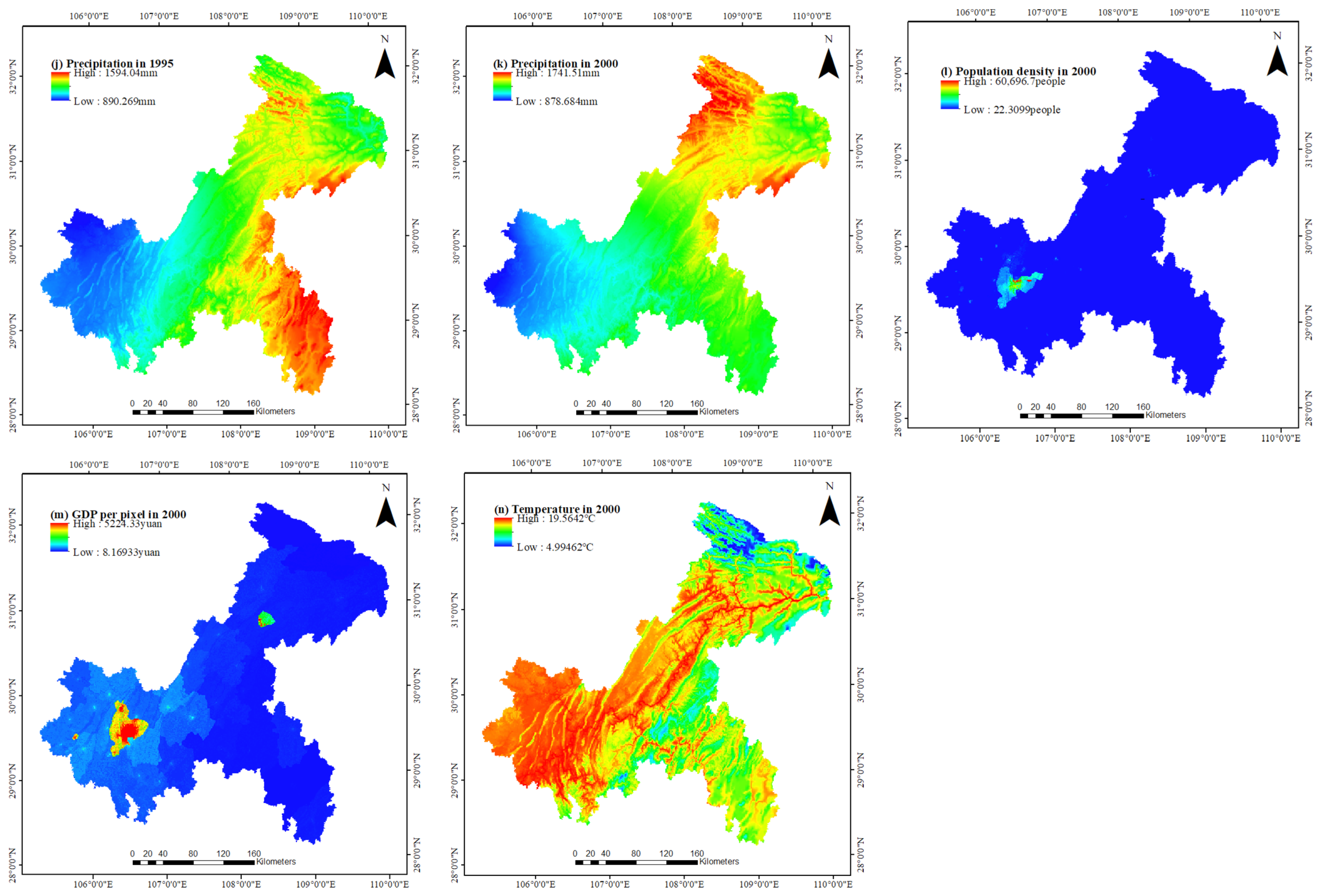
2.3.2. Scenario Definitions and Driving Factors
2.3.3. Markov Chain Model
2.3.4. FLUS Model
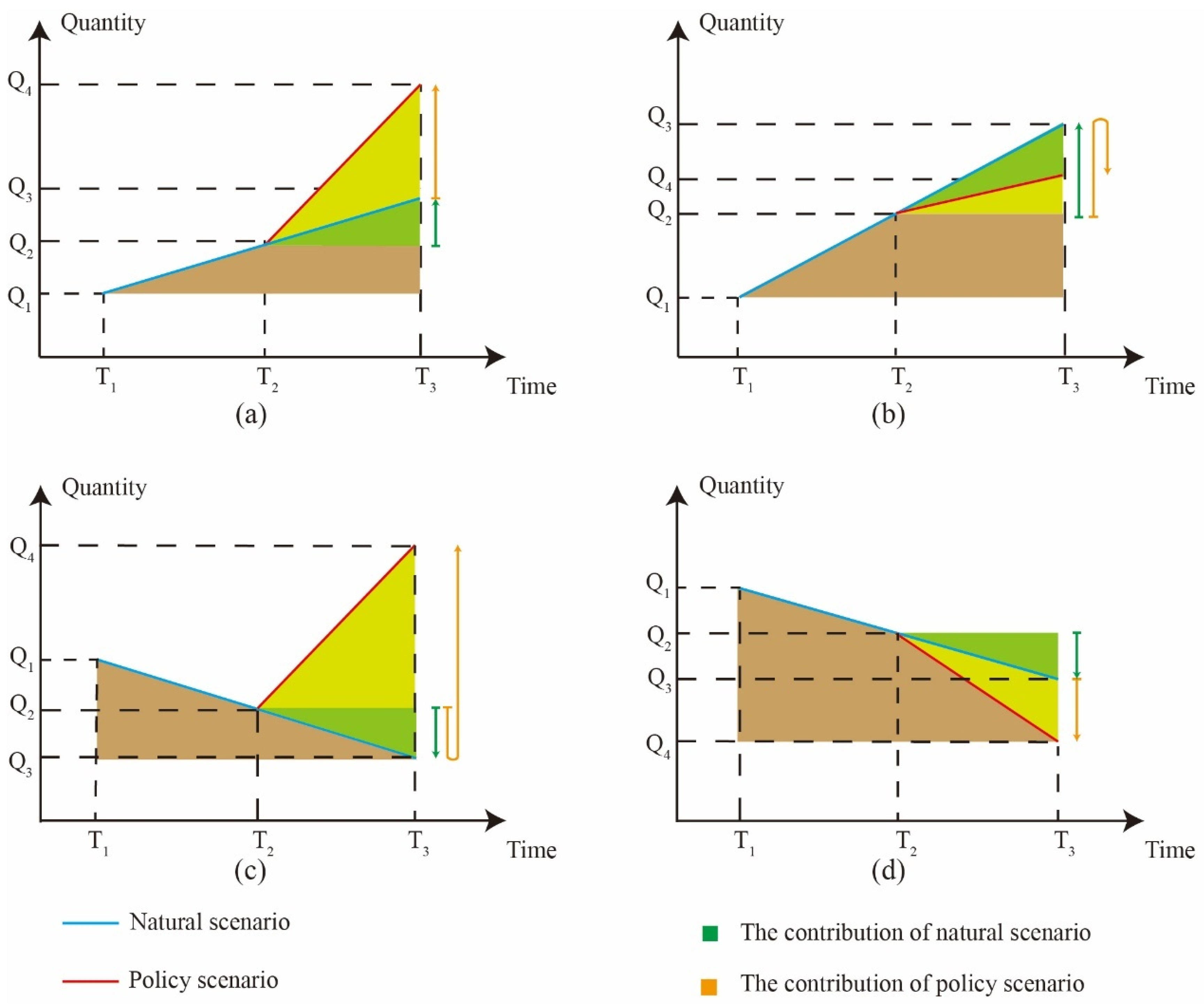
2.3.5. Relative Contribution Conceptual Model (RCCM)
2.3.6. Complex Network Model
- (1)
- Node degree
- (2)
- Betweenness centrality
- (3)
- Average shortest path length
2.3.7. Urban Expansion Elasticity Factor
3. Results
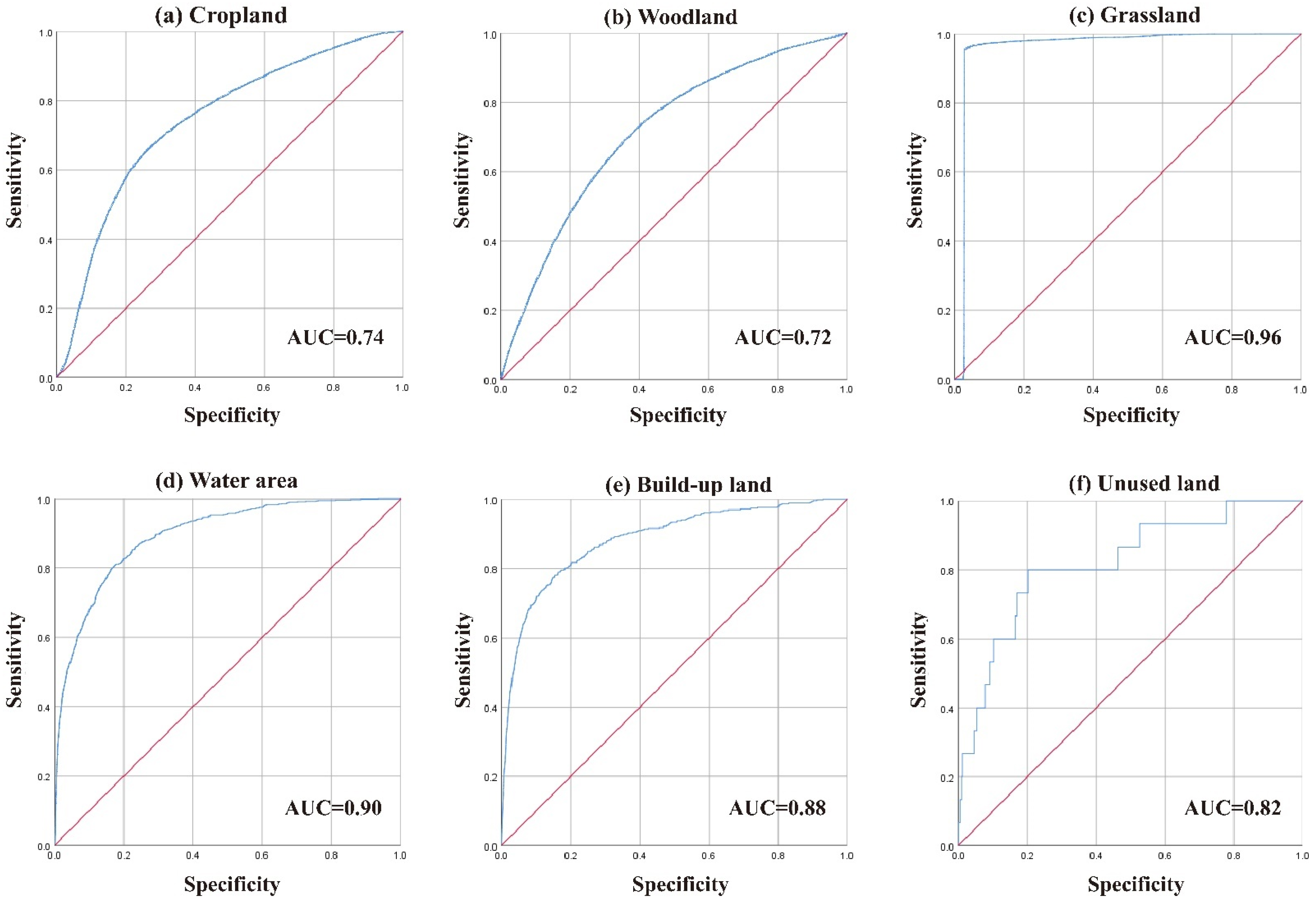
3.1. Simulation Accuracy Evaluation
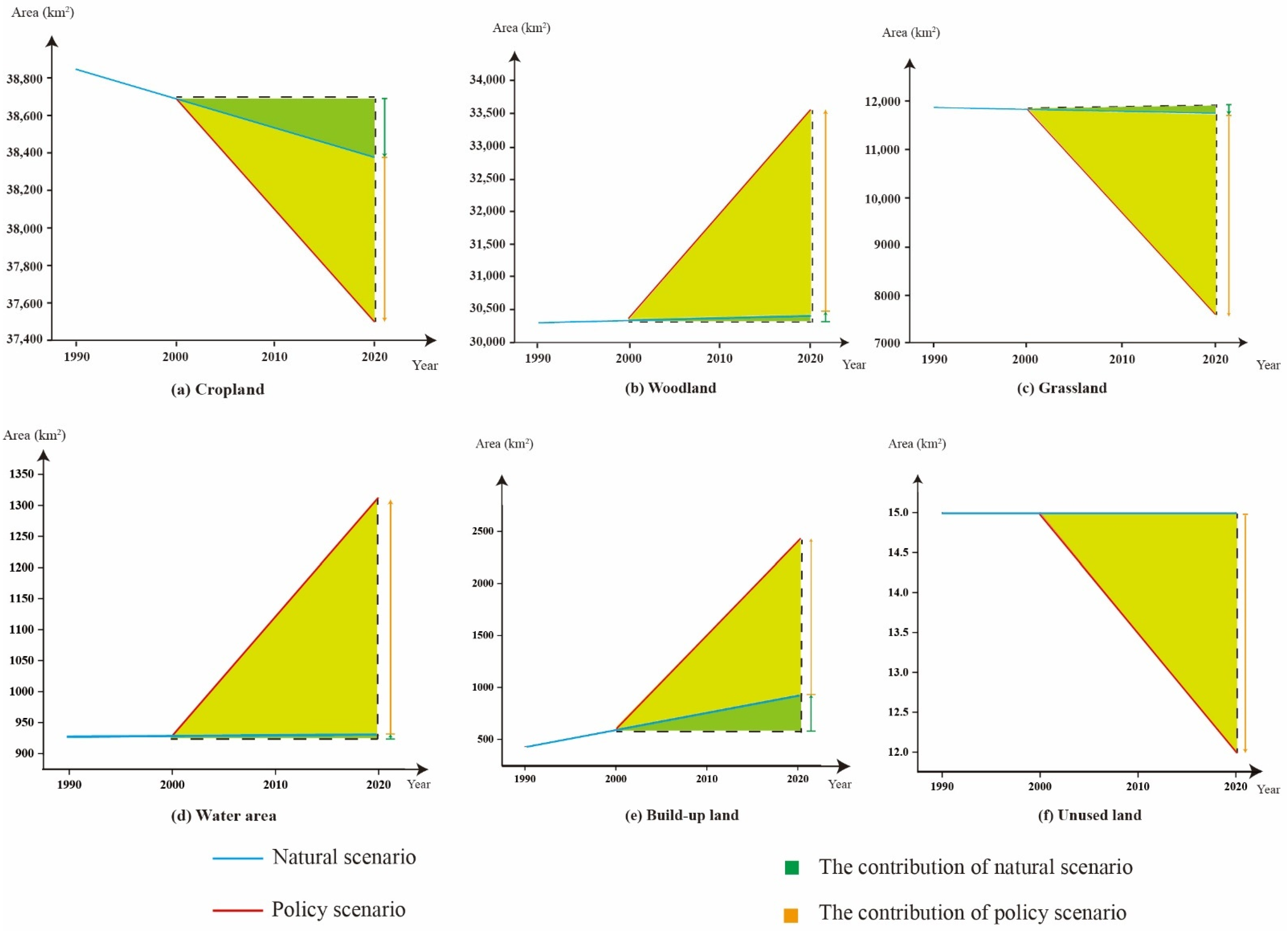
3.2. The Relative Contributions of Natural and Policy Contexts to LUCC
3.3. LUCC between 1990–2000 and 2000–2020
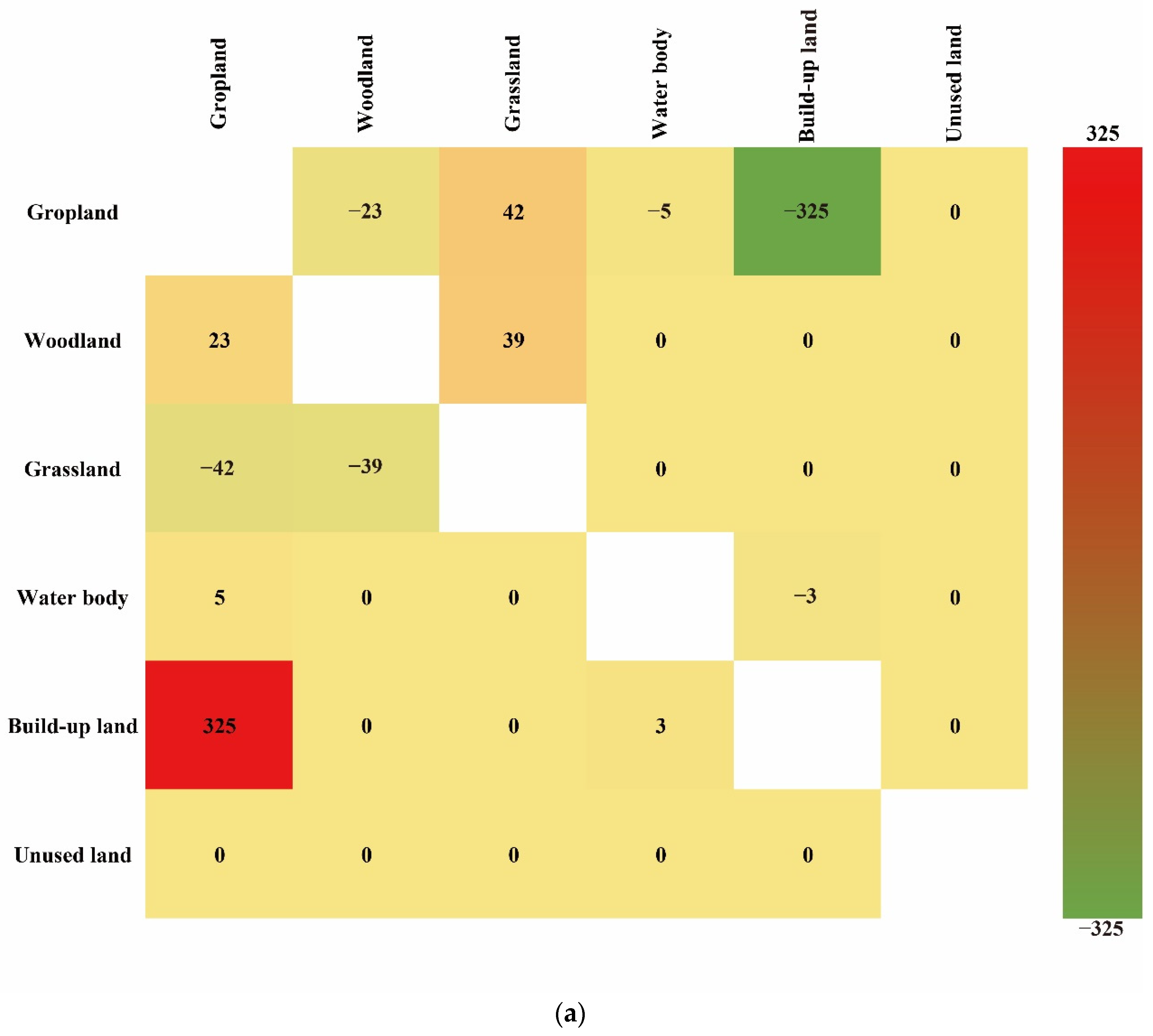
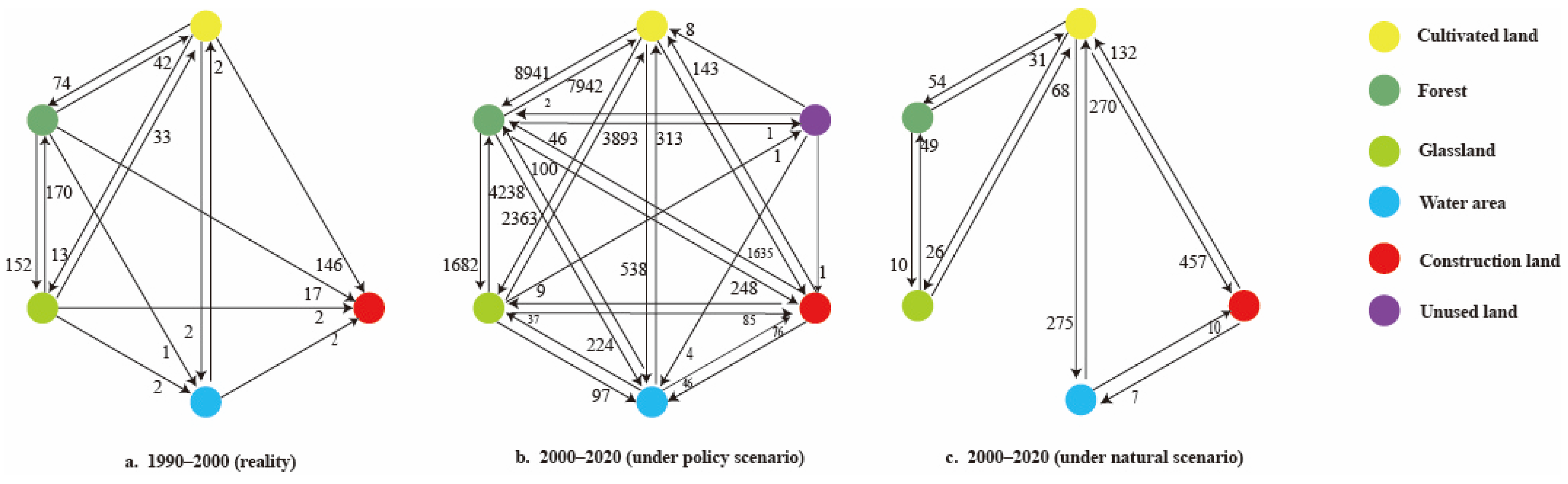
3.4. Analysis of Land Use Changes Based on Complex Network Models
3.5. Coordination Analysis of Urban Expansion and Population Development in Chongqing
4. Discussion
4.1. The Three Gorges Dam Project (TGDP)
4.2. China’s Western Development Strategy
4.3. Economical and Intensive Land Use
4.4. The Grain for Green Program (GFGP)
5. Policy Implications
5.1. Promotion of Natural Forest Restoration
5.2. Local Conditions Should Be Considered When Afforestation Occurs
5.3. Efficient Use of Construction Land and Protection of Agricultural Land
6. Conclusions
Author Contributions
Funding
Data Availability Statement
Conflicts of Interest
Appendix A
References
- Grimm, N.B.; Faeth, S.H.; Golubiewski, N.E.; Redman, C.L.; Wu, J.G.; Bai, X.M.; Briggs, J.M. Global change and the ecology of cities. Science 2008, 319, 756–760. [Google Scholar] [CrossRef] [PubMed] [Green Version]
- Gardner, A.S.; Moholdt, G.; Wouters, B.; Wolken, G.J.; Burgess, D.O.; Sharp, M.J.; Cogley, J.G.; Braun, C.; Labine, C. Sharply increased mass loss from glaciers and ice caps in the Canadian Arctic Archipelago. Nature 2011, 473, 357–360. [Google Scholar] [CrossRef] [PubMed]
- Khanna, J.; Medvigy, D.; Fueglistaler, S.; Walko, R. Regional dry-season climate changes due to three decades of Amazonian deforestation. Nat. Clim. Chang. 2017, 7, 200–204. [Google Scholar] [CrossRef]
- Sterling, S.M.; Ducharne, A.; Polcher, J. The impact of global land-cover change on the terrestrial water cycle. Nat. Clim. Chang. 2013, 3, 385–390. [Google Scholar] [CrossRef]
- Zhao, H.F.; He, H.M.; Wang, J.J.; Bai, C.Y.; Zhang, C.J. Vegetation Restoration and Its Environmental Effects on the Loess Plateau. Sustainability 2018, 10, 4676. [Google Scholar] [CrossRef] [Green Version]
- Wang, H.; Ni, J.; Prentice, I.C. Sensitivity of potential natural vegetation in China to projected changes in temperature, precipitation and atmospheric CO2. Reg. Environ. Chang. 2011, 11, 715–727. [Google Scholar] [CrossRef] [Green Version]
- Kirwan, M.L.; Guntenspergen, G.R.; D’Alpaos, A.; Morris, J.T.; Mudd, S.M.; Temmerman, S. Limits on the adaptability of coastal marshes to rising sea level. Geophys. Res. Lett. 2010, 37, L23401. [Google Scholar] [CrossRef] [Green Version]
- Vina, A.; McConnell, W.J.; Yang, H.B.; Xu, Z.C.; Liu, J.G. Effects of conservation policy on China’s forest recovery. Sci. Adv. 2016, 2, e1500965. [Google Scholar] [CrossRef] [Green Version]
- Meyer, W.B.; Turner, B.L. Human-Population Growth and Global Land-Use Cover Change. Annu. Rev. Ecol. Syst. 1992, 23, 39–61. [Google Scholar] [CrossRef]
- Liu, Y.S.; Li, J.T.; Yang, Y.Y. Strategic adjustment of land use policy under the economic transformation. Land Use Policy 2018, 74, 5–14. [Google Scholar] [CrossRef]
- Barsimantov, J.; Antezana, J.N. Forest cover change and land tenure change in Mexico’s avocado region: Is community forestry related to reduced deforestation for high value crops? Appl. Geogr. 2012, 32, 844–853. [Google Scholar] [CrossRef]
- Nesheim, I.; Reidsma, P.; Bezlepkina, I.; Verburg, R.; Abdeladhim, M.A.; Bursztyn, M.; Chen, L.; Cisse, Y.; Feng, S.Y.; Gicheru, P.; et al. Causal chains, policy trade offs and sustainability: Analysing land (mis)use in seven countries in the South. Land Use Policy 2014, 37, 60–70. [Google Scholar] [CrossRef]
- Liu, J.G.; Li, S.X.; Ouyang, Z.Y.; Tam, C.; Chen, X.D. Ecological and socioeconomic effects of China’s policies for ecosystem services. Proc. Natl. Acad. Sci. USA 2008, 105, 9477–9482. [Google Scholar] [CrossRef] [Green Version]
- Li, G.; Sun, S.B.; Han, J.C.; Yan, J.W.; Liu, W.B.; Wei, Y.; Lu, N.; Sun, Y.Y. Impacts of Chinese Grain for Green program and climate change on vegetation in the Loess Plateau during 1982–2015 (vol 660, pg 177, 2019). Sci. Total Environ. 2019, 665, 1190–1191. [Google Scholar] [CrossRef]
- Erjavec, E.; Lovec, M. Research of European Union’s Common Agricultural Policy: Disciplinary boundaries and beyond. Eur Rev. Agric. Econ. 2017, 44, 732–754. [Google Scholar] [CrossRef]
- Feng, X.M.; Fu, B.J.; Piao, S.; Wang, S.H.; Ciais, P.; Zeng, Z.Z.; Lu, Y.H.; Zeng, Y.; Li, Y.; Jiang, X.H.; et al. Revegetation in China’s Loess Plateau is approaching sustainable water resource limits. Nat. Clim Chang. 2016, 6, 1019–1022. [Google Scholar] [CrossRef]
- Tian, H.J.; Cao, C.X.; Chen, W.; Bao, S.N.; Yang, B.; Myneni, R.B. Response of vegetation activity dynamic to climatic change and ecological restoration programs in Inner Mongolia from 2000 to 2012. Ecol. Eng. 2015, 82, 276–289. [Google Scholar] [CrossRef]
- Van Den Hoek, J.; Ozdogan, M.; Burnicki, A.; Zhu, A.X. Evaluating forest policy implementation effectiveness with a cross-scale remote sensing analysis in a priority conservation area of Southwest China. Appl. Geogr. 2014, 47, 177–189. [Google Scholar] [CrossRef]
- Fu, Q.; Hou, Y.; Wang, B.; Bi, X.; Li, B.; Zhang, X.S. Scenario analysis of ecosystem service changes and interactions in a mountain-oasis-desert system: A case study in Altay Prefecture, China. Sci. Rep. 2018, 8, 12939. [Google Scholar] [CrossRef] [PubMed]
- Baker, W.L. A review of models of landscape change. Landsc. Ecol. 1989, 2, 112–134. [Google Scholar] [CrossRef]
- Overmars, K.P.; de Koning, G.H.J.; Veldkamp, A. Spatial autocorrelation in multi-scale land use models. Ecol. Model. 2003, 164, 257–270. [Google Scholar] [CrossRef]
- Yang, Y.Y.; Bao, W.K.; Liu, Y.S. Scenario simulation of land system change in the Beijing-Tianjin-Hebei region. Land Use Policy 2020, 96, 12. [Google Scholar] [CrossRef]
- Zhou, L.; Dang, X.W.; Sun, Q.K.; Wang, S.H. Multi-scenario simulation of urban land change in Shanghai by random forest and CA-Markov model. Sust. Cities Soc. 2020, 55, 10. [Google Scholar] [CrossRef]
- Chen, Y.M.; Li, X.; Wang, S.J.; Liu, X.P. Defining agents’ behaviour based on urban economic theory to simulate complex urban residential dynamics. Int. J. Geogr. Inf. Sci. 2012, 26, 1155–1172. [Google Scholar] [CrossRef]
- Tang, F.; Fu, M.C.; Wang, L.; Zhang, P.T. Land-use change in Changli County, China: Predicting its spatio-temporal evolution in habitat quality. Ecol. Indic. 2020, 117, 8. [Google Scholar] [CrossRef]
- Liu, X.P.; Liang, X.; Li, X.; Xu, X.C.; Ou, J.P.; Chen, Y.M.; Li, S.Y.; Wang, S.J.; Pei, F.S. A future land use simulation model (FLUS) for simulating multiple land use scenarios by coupling human and natural effects. Landsc. Urban Plan. 2017, 168, 94–116. [Google Scholar] [CrossRef]
- Du, X.Z.; Zhao, X.; Liang, S.L.; Zhao, J.C.; Xu, P.P.; Wu, D.H. Quantitatively Assessing and Attributing Land Use and Land Cover Changes on China’s Loess Plateau. Remote Sens. 2020, 12, 353. [Google Scholar] [CrossRef] [Green Version]
- Liu, X.P.; Wang, S.J.; Wu, P.J.; Feng, K.S.; Hubacek, K.; Li, X.; Sun, L.X. Impacts of Urban Expansion on Terrestrial Carbon Storage in China. Environ. Sci. Technol. 2019, 53, 6834–6844. [Google Scholar] [CrossRef]
- Liang, X.; Liu, X.P.; Li, X.; Chen, Y.M.; Tian, H.; Yao, Y. Delineating multi-scenario urban growth boundaries with a CA-based FLUS model and morphological method. Landsc. Urban Plan. 2018, 177, 47–63. [Google Scholar] [CrossRef]
- Zhou, R.; Zhang, H.; Ye, X.Y.; Wang, X.J.; Su, H.L. The Delimitation of Urban Growth Boundaries Using the CLUE-S Land-Use Change Model: Study on Xinzhuang Town, Changshu City, China. Sustainability 2016, 8, 1182. [Google Scholar] [CrossRef] [Green Version]
- Xu, H.T.; Song, Y.C.; Tian, Y. Simulation of land-use pattern evolution in hilly mountainous areas of North China: A case study in Jincheng. Land Use Policy 2022, 112, 14. [Google Scholar] [CrossRef]
- Deng, Y.; Yao, S.; Hou, M.; Zhang, T.; Lu, Y.; Gong, Z.; Wang, Y. Assessing the effects of the Green for Grain Program on ecosystem carbon storage service by linking the InVEST and FLUS models: A case study of Zichang county in hilly and gully region of Loess Plateau. J. Nat. Resour. 2020, 35, 826–844. [Google Scholar]
- Dan, W.; Wei, H.; Zhang, S.W.; Kun, B.; Bao, X.; Yi, W.; Yue, L. Processes and prediction of land use/land cover changes (LUCC) driven by farm construction: The case of Naoli River Basin in Sanjiang Plain. Environ. Earth Sci. 2015, 73, 4841–4851. [Google Scholar] [CrossRef]
- Wang, S.Y.; Cheng, W.Y.; Mei, G. Efficient Method for Improving the Spreading Efficiency in Small-World Networks and Assortative Scale-Free Networks. IEEE Access 2019, 7, 46122–46134. [Google Scholar] [CrossRef]
- Wang, L.S.; Song, R.; Qu, Z.; Zhao, H.; Zhai, C.M. Study of China’s Publicity Translations Based on Complex Network Theory. IEEE Access 2018, 6, 35753–35763. [Google Scholar] [CrossRef]
- Li, X.; Chen, G.Z.; Liu, X.P.; Liang, X.; Wang, S.J.; Chen, Y.M.; Pei, F.S.; Xu, X.C. A New Global Land-Use and Land-Cover Change Product at a 1-km Resolution for 2010 to 2100 Based on Human-Environment Interactions. Ann. Am. Assoc. Geogr. 2017, 107, 1040–1059. [Google Scholar] [CrossRef]
- Hanley, J.A.; McNeil, B.J. The meaning and use of the area under a receiver operating characteristic (ROC) curve. Radiology 1982, 143, 29–36. [Google Scholar] [CrossRef] [Green Version]
- Moghadam, H.S.; Helbich, M. Spatiotemporal urbanization processes in the megacity of Mumbai, India: A Markov chains-cellular automata urban growth model. Appl. Geogr. 2013, 40, 140–149. [Google Scholar] [CrossRef]
- Veldkamp, A.; Lambin, E.F. Predicting land-use change. Agric. Ecosyst. Environ. 2001, 85, 1–6. [Google Scholar] [CrossRef]
- Fischer, G.; Sun, L.X. Model based analysis of future land-use development in China. Agric. Ecosyst. Environ. 2001, 85, 163–176. [Google Scholar] [CrossRef]
- Hu, Y.F.; Batunacun; Zhen, L.; Zhuang, D.F. Assessment of Land-Use and Land-Cover Change in Guangxi, China. Sci. Rep. 2019, 9, 2189. [Google Scholar] [CrossRef] [PubMed] [Green Version]
- Al-sharif, A.A.A.; Pradhan, B. Monitoring and predicting land use change in Tripoli Metropolitan City using an integrated Markov chain and cellular automata models in GIS. Arab. J. Geosci. 2014, 7, 4291–4301. [Google Scholar] [CrossRef]
- Yang, W.T.; Long, D.; Bai, P. Impacts of future land cover and climate changes on runoff in the mostly afforested river basin in North China. J. Hydrol. 2019, 570, 201–219. [Google Scholar] [CrossRef]
- Yang, X.; Zheng, X.Q.; Chen, R. A land use change model: Integrating landscape pattern indexes and Markov-CA. Ecol. Model. 2014, 283, 1–7. [Google Scholar] [CrossRef]
- Guan, D.J.; Li, H.F.; Inohae, T.; Su, W.C.; Nagaie, T.; Hokao, K. Modeling urban land use change by the integration of cellular automaton and Markov model. Ecol. Model. 2011, 222, 3761–3772. [Google Scholar] [CrossRef]
- Dong, N.; You, L.; Cai, W.J.; Li, G.; Lin, H. Land use projections in China under global socioeconomic and emission scenarios: Utilizing a scenario-based land-use change assessment framework. Glob. Environ. Chang. 2018, 50, 164–177. [Google Scholar] [CrossRef]
- Feng, D.R.; Bao, W.K.; Fu, M.C.; Zhang, M.; Sun, Y.Y. Current and Future Land Use Characters of a National Central City in Eco-Fragile Region-A Case Study in Xi’an City Based on FLUS Model. Land 2021, 10, 286. [Google Scholar] [CrossRef]
- Newman, M.E.J. The structure and function of complex networks. SIAM Rev. 2003, 45, 167–256. [Google Scholar] [CrossRef] [Green Version]
- Dorogovtsev, S.N.; Mendes, J.F.F. Evolution of networks. Adv. Phys. 2002, 51, 1079–1187. [Google Scholar] [CrossRef] [Green Version]
- Poisot, T.; Gravel, D. When is an ecological network complex? Connectance drives degree distribution and emerging network properties. PeerJ 2014, 2, e251. [Google Scholar] [CrossRef] [PubMed] [Green Version]
- Purbosari, K. Exploring the Roles of Social Networks Centrality in Indonesian Public Employees: Degree, Betweenness and Closeness. In Proceedings of the Third International Conference on Asian Studies 2015, Niigata, Japan, 20–21 June 2015; p. 20. [Google Scholar]
- Zhang, Z.T.; Wang, J.M.; Li, B. Determining the influence factors of soil organic carbon stock in opencast coal-mine dumps based on complex network theory. Catena 2019, 173, 433–444. [Google Scholar] [CrossRef]
- Newman, M.E.J. A measure of betweenness centrality based on random walks. Soc. Netw. 2005, 27, 39–54. [Google Scholar] [CrossRef] [Green Version]
- Brandes, U. A faster algorithm for betweenness centrality. J. Math. Sociol. 2001, 25, 163–177. [Google Scholar] [CrossRef]
- Wang, Y.; Li, X.M.; Li, J.F.; Huang, Z.D.; Xiao, R.B. Impact of Rapid Urbanization on Vulnerability of Land System from Complex Networks View: A Methodological Approach. Complexity 2018, 2018, 8561675. [Google Scholar] [CrossRef] [Green Version]
- Qian, W.; Zengxiang, Z.; Ling, Y.I.; Wenbin, T.A.N.; Changyou, W. Research on Urban Expansion in Nanjing, China Using RS and GIS. Resour. Environ. Yangtze Basin 2007, 16, 554–559. [Google Scholar]
- Liu, Y.; Deng, X.; Gan, H. The State and Optimization Countermeasures of Urban Land- use in China. J. Chongqing Jianzhu Univ. 2005, 27, 1–4. [Google Scholar]
- Zhang, M.; Wang, J.M.; Feng, Y. Temporal and spatial change of land use in a large-scale opencast coal mine area: A complex network approach. Land Use Policy 2019, 86, 375–386. [Google Scholar] [CrossRef]
- Liu, Y.S.; Fang, F.; Li, Y.H. Key issues of land use in China and implications for policy making. Land Use Policy 2014, 40, 6–12. [Google Scholar] [CrossRef]
- New, T.; Xie, Z. Impacts of large dams on riparian vegetation: Applying global experience to the case of China’s Three Gorges Dam. Biodivers. Conserv. 2008, 17, 3149–3163. [Google Scholar] [CrossRef]
- Ponseti, M.; Pujol, J.L. The Three Gorges Dam Project in China: History and consequences. HMiC Història Mod. Contemp. 2006, 4, 151–188. [Google Scholar]
- Liu, J.Y.; Kuang, W.H.; Zhang, Z.X.; Xu, X.L.; Qin, Y.W.; Ning, J.; Zhou, W.C.; Zhang, S.W.; Li, R.D.; Yan, C.Z.; et al. Spatiotemporal characteristics, patterns, and causes of land-use changes in China since the late 1980s. J. Geogr. Sci. 2014, 24, 195–210. [Google Scholar] [CrossRef]
- Long, H.; Wu, X.; Wang, W.; Dong, G. Analysis of urban-rural land-use change during 1995–2006 and its policy dimensional driving forces in Chongqing, China. Sensors 2008, 8, 681–699. [Google Scholar] [CrossRef] [PubMed] [Green Version]
- Lamb, D.; Erskine, P.D.; Parrotta, J.A. Restoration of degraded tropical forest landscapes. Science 2005, 310, 1628–1632. [Google Scholar] [CrossRef] [Green Version]
- Lu, Q.S.; Xu, B.; Liang, F.Y.; Gao, Z.Q.; Ning, J.C. Influences of the Grain-for-Green project on grain security in southern China. Ecol. Indic. 2013, 34, 616–622. [Google Scholar] [CrossRef] [Green Version]
- Feng, D.R.; Bao, W.K.; Yang, Y.Y.; Fu, M.C. How do government policies promote greening? Evidence from China. Land Use Policy 2021, 104, 105389. [Google Scholar] [CrossRef]
- Chazdon, R.L. Beyond deforestation: Restoring forests and ecosystem services on degraded lands. Science 2008, 320, 1458–1460. [Google Scholar] [CrossRef] [Green Version]
- McVicar, T.R.; Van Niel, T.G.; Li, L.T.; Wen, Z.M.; Yang, Q.K.; Li, R.; Jiao, F. Parsimoniously modelling perennial vegetation suitability and identifying priority areas to support China’s re-vegetation program in the Loess Plateau: Matching model complexity to data availability. Forest Ecol. Manag. 2010, 259, 1277–1290. [Google Scholar] [CrossRef]
- Normile, D. Ecology-Getting at the roots of killer dust storms. Science 2007, 317, 314–316. [Google Scholar] [CrossRef]
- Asner, G.P.; Hughes, R.F.; Vitousek, P.M.; Knapp, D.E.; Kennedy-Bowdoin, T.; Boardman, J.; Martin, R.E.; Eastwood, M.; Green, R.O. Invasive plants transform the three-dimensional structure of rain forests. Proc. Natl. Acad. Sci. USA 2008, 105, 4519–4523. [Google Scholar] [CrossRef] [Green Version]
- Cao, S.X.; Wang, G.S.; Chen, L. Questionable value of planting thirsty trees in dry regions. Nature 2010, 465, 31. [Google Scholar] [CrossRef] [PubMed] [Green Version]
- Cao, S.X.; Chen, L.; Shankman, D.; Wang, C.M.; Wang, X.B.; Zhang, H. Excessive reliance on afforestation in China’s arid and semi-arid regions: Lessons in ecological restoration. Earth-Sci. Rev. 2011, 104, 240–245. [Google Scholar] [CrossRef]
- Song, X.P.; Hansen, M.C.; Stehman, S.V.; Potapov, P.V.; Tyukavina, A.; Vermote, E.F.; Townshend, J.R. Global land change from 1982 to 2016 (vol 560, pg 639, 2018). Nature 2018, 563, E26. [Google Scholar] [CrossRef] [Green Version]
- Chen, M.X.; Liu, W.D.; Lu, D.D. Challenges and the way forward in China’s new-type urbanization. Land Use Policy 2016, 55, 334–339. [Google Scholar] [CrossRef]
- Long, H.L.; Li, Y.R.; Liu, Y.S.; Woods, M.; Zou, J. Accelerated restructuring in rural China fueled by ‘increasing vs. decreasing balance’ land-use policy for dealing with hollowed villages. Land Use Policy 2012, 29, 11–22. [Google Scholar] [CrossRef]


| Category | Data | Spatial Resolution | Data Resource |
|---|---|---|---|
| Terrain | Aspect | 1000 m | Calculated according to DEM |
| Slope | 1000 m | Calculated according to DEM | |
| Soil | Silt | CAS (http://www.resdc.cn (accessed on 10 January 2022)) | |
| Temperature | Annual average temperature | 1000 m | CAS (http://www.resdc.cn (accessed on 10 January 2022)) |
| Precipitation | Annual precipitation | 1000 m | CAS (http://www.resdc.cn (accessed on 10 January 2022)) |
| Human influence | Population density | 1000 m | CAS (http://www.resdc.cn (accessed on 10 January 2022)) |
| GDP | 1000 m | CAS (http://www.resdc.cn (accessed on 10 January 2022)) | |
| Distance to railway | Vector | GDEMDEM (http://www.gscloud.cn/ (accessed on 10 January 2022)) | |
| Distance to road | Vector | GDEMDEM (http://www.gscloud.cn/ (accessed on 10 January 2022)) | |
| Distance to residential area | Vector | GDEMDEM (http://www.gscloud.cn/ (accessed on 10 January 2022)) |
| Producer Accuracy | User Accuracy | Kappa Coefficient | Overall Accuracy | |
|---|---|---|---|---|
| Cultivated land | 0.990254 | 0.993056 | 0.978426 | 0.986650 |
| Forest | 0.991205 | 0.987987 | ||
| Grassland | 0.980322 | 0.974222 | ||
| Water area | 0.988095 | 1 | ||
| Construction land | 0.726471 | 0.730159 | ||
| Unused land | 1 | 1 |
| Cultivated Land | Forest | Grassland | Water Area | Construction Land | Unused Land | |
|---|---|---|---|---|---|---|
| Policy background | 37,504 | 33,575 | 7608 | 1312 | 2399 | 12 |
| Natural background | 38,381 | 30,407 | 11,747 | 929 | 925 | 15 |
| Scenario | Cultivated Land | Forest | Grassland | Water Area | Construction Land | Unused Land | Losses * | |
|---|---|---|---|---|---|---|---|---|
| 1990–2000 (reality) | Cultivated land | 38,615 | 74 | 13 | 2 | 146 | 0 | 235 |
| Forest | 42 | 30,101 | 152 | 1 | 17 | 0 | 212 | |
| Grassland | 33 | 170 | 11,663 | 2 | 2 | 0 | 207 | |
| Water area | 2 | 0 | 0 | 922 | 2 | 0 | 4 | |
| Construction land | 0 | 0 | 0 | 0 | 430 | 0 | 0 | |
| Unused land | 0 | 0 | 0 | 0 | 0 | 15 | 0 | |
| Gains * | 77 | 244 | 165 | 5 | 167 | 0 | ||
| 2000–2020 (under policy scenarios) | Cultivated land | 25,172 | 8941 | 2363 | 538 | 1635 | 10 | 13,487 |
| Forest | 7942 | 20,207 | 1682 | 224 | 248 | 1 | 10,097 | |
| Grassland | 3893 | 4238 | 3501 | 97 | 85 | 1 | 8314 | |
| Water area | 313 | 100 | 37 | 400 | 76 | 0 | 526 | |
| Construction land | 143 | 46 | 9 | 46 | 353 | 0 | 244 | |
| Unused land | 8 | 2 | 0 | 4 | 1 | 0 | 15 | |
| Gains * | 12,299 | 13,327 | 4091 | 909 | 2045 | 12 | ||
| 2000–2020 (under natural scenarios) | Cultivated land | 37,880 | 54 | 26 | 275 | 457 | 0 | 812 |
| Forest | 31 | 30,304 | 10 | 0 | 0 | 0 | 41 | |
| Grassland | 68 | 49 | 11,711 | 0 | 0 | 0 | 117 | |
| Water area | 270 | 0 | 0 | 647 | 10 | 0 | 280 | |
| Construction land | 132 | 0 | 0 | 7 | 458 | 0 | 139 | |
| Unused land | 0 | 0 | 0 | 0 | 0 | 15 | 0 | |
| Gains * | 501 | 103 | 36 | 282 | 467 | 0 |
| Cultivated Land | Forest | Grassland | Water Area | Construction Land | Unused Land | |
|---|---|---|---|---|---|---|
| Policy background | 36,861 | 34,000 | 6548 | 1557 | 3427 | 12 |
| Scenario | Land Use Types | Output Degree | Input Degree | Output Degree/Input Degree |
|---|---|---|---|---|
| 1990–2000 (reality) | Cultivated land | 38,850 | 38,692 | 1.004 |
| Forest | 30,313 | 30,345 | 0.999 | |
| Grassland | 11,870 | 11,828 | 1.004 | |
| Water area | 926 | 927 | 0.999 | |
| Construction land | 430 | 597 | 0.720 | |
| Unused land | 15 | 15 | 1.000 | |
| 2000–2020 (under policy scenarios) | Cultivated land | 38,659 | 37,464 | 1.032 |
| Forest | 30,304 | 33,534 | 0.904 | |
| Grassland | 11,815 | 7592 | 1.556 | |
| Water area | 926 | 1309 | 0.707 | |
| Construction land | 597 | 2398 | 0.249 | |
| Unused land | 8 | 12 | 0.667 | |
| 2000–2020 (under natural scenarios) | Cultivated land | 38,692 | 38,381 | 1.008 |
| Forest | 30,345 | 30,407 | 0.998 | |
| Grassland | 11,828 | 11,747 | 1.007 | |
| Water area | 927 | 929 | 0.998 | |
| Construction land | 597 | 925 | 0.645 | |
| Unused land | 15 | 15 | 1.000 |
| Land Use Type | 1990–2000 | 2000–2020 (Policy Background) | 2000–2020 (Natural Background) |
|---|---|---|---|
| Cultivated land | 2.00 | 0.92 | 8.0 |
| Forest | 0.00 | 0.92 | 0.0 |
| Grassland | 0.00 | 0.67 | 0.0 |
| Water area | 0.00 | 0.25 | 0.0 |
| Construction land | 0.00 | 0.25 | 0.0 |
| Unused land | 0.00 | 0.00 | 0.0 |
| Land Use Type | 1990–2000 | 2000–2020 (Policy Background) | 2000–2020 (Natural Background) |
|---|---|---|---|
| Cultivated land | 9 | 12 | 10 |
| Forest | 8 | 12 | 6 |
| Grassland | 8 | 11 | 6 |
| Water area | 7 | 11 | 6 |
| Construction land | 6 | 11 | 6 |
| Unused land | 2 | 7 | 2 |
| Average node degree | 3.333 | 5.33 | 3 |
| Period | Average Shortest Path |
|---|---|
| 1990–2000 | 1.125 |
| 2000–2020 (Policy background) | 1.1 |
| 2000–2020 (Natural background) | 1.4 |
| 2006 | 2010 | 2015 | 2020 | |
|---|---|---|---|---|
| Built-up area | 631.35 | 870.23 | 1329.45 | 1565.61 |
| City population | 747.02 | 831.69 | 1032.63 | 1213.56 |
| Average Annual Growth Rate of Urban Built-Up Area (%) | Average Annual Urban Population Growth Rate (%) | Elasticity Factor | |
|---|---|---|---|
| 2006–2010 | 9.46 | 2.83 | 3.34 |
| 2010–2015 | 10.55 | 4.83 | 2.18 |
| 2015–2020 | 3.55 | 3.50 | 1.01 |
| 2006–2020 | 10.57 | 4.46 | 2.37 |
Publisher’s Note: MDPI stays neutral with regard to jurisdictional claims in published maps and institutional affiliations. |
© 2022 by the authors. Licensee MDPI, Basel, Switzerland. This article is an open access article distributed under the terms and conditions of the Creative Commons Attribution (CC BY) license (https://creativecommons.org/licenses/by/4.0/).
Share and Cite
Zuo, Y.; Cheng, J.; Fu, M. Analysis of Land Use Change and the Role of Policy Dimensions in Ecologically Complex Areas: A Case Study in Chongqing. Land 2022, 11, 627. https://doi.org/10.3390/land11050627
Zuo Y, Cheng J, Fu M. Analysis of Land Use Change and the Role of Policy Dimensions in Ecologically Complex Areas: A Case Study in Chongqing. Land. 2022; 11(5):627. https://doi.org/10.3390/land11050627
Chicago/Turabian StyleZuo, Yiting, Jie Cheng, and Meichen Fu. 2022. "Analysis of Land Use Change and the Role of Policy Dimensions in Ecologically Complex Areas: A Case Study in Chongqing" Land 11, no. 5: 627. https://doi.org/10.3390/land11050627