1. Introduction
“If the nation is to be revitalized, the countryside must be revitalized”, the explanation of General Secretary Xi Jinping about China’s agriculture and rural areas shows the importance of agricultural and rural work to China’s development [
1]. Judging from the global development experience, agriculture is an important cornerstone of national security and stability [
2]. Agricultural ecological efficiency (AEE) refers to the exchange of less natural resource consumption and environmental costs for more quantities and higher quality of agricultural products or agricultural services within the affordability of the ecosystem [
3,
4]. Since the reform and opening-up in 1978, based on the production model of petroleum agriculture, the agricultural output level in China has witnessed a continuous growth [
5], but it has also paid a high price for resources and the environment [
6]. Since 1978, China has made great achievements in agricultural development [
7]. In 2021, the total grain output of China reached 683 million tons, increasing by 2% over the previous year. The annual grain output reached a new high level, maintaining more than 0.665 trillion kg for seven consecutive years. In 2015, the Ministry of Agriculture and Rural Affairs organized a zero-growth action for the use of chemical fertilizers and pesticides, and by the end of 2020, the reduction and efficiency improvement of chemical fertilizers and pesticides in China had successfully achieved the expected goals [
8]. The use of chemical fertilizers and pesticides has been significantly reduced [
9], while their utilization rate has been significantly improved, and the effect of promoting high-quality development of the planting industry was obvious [
10]. In 2020, formula fertilizer accounted for more than 60% of the total application of the three major grain crops, the area of mechanical fertilization exceeded 46.66 million hectares, and the integration of water and fertilizer exceeded 9.33 million hectares. In addition, the green prevention and control area covered nearly 66.66 million hectares, and the green prevention and control rate of major crop diseases and insect pests was 41.5% in 2020, 18.5% higher than that in 2015. However, the green development of agriculture is still the main theme of the current agricultural development [
11]. In the context of tightening resource and environmental constraints, the balance between economic and ecological benefits of agricultural development has become a major challenge facing China [
12].
The green development of agriculture needs to clarify the relationship between agricultural input and output [
13] and resource consumption and environmental protection [
14], so it is necessary to consider the ecological externalities generated by agriculture in the measurement of input-output processes [
15] and use key indicators of ecological efficiency to measure the production efficiency of agriculture [
16]. The concept of eco-efficiency was proposed by German scholars [
17], promoted by the World Business Council for Sustainable Development and the OECD, and recognized by scholars and governments [
18]. The specific embodiment of the concept of agricultural ecological efficiency is to obtain as much agricultural output as possible with the smallest possible resource consumption and environmental pollution [
19] and to ensure the quality of agricultural products [
20]. Based on the concept of agricultural production efficiency, it not only needs to pay attention to maximizing agricultural economic benefits (desirable output) [
21], but also minimizing resource consumption and environmental damage (undesirable output) to conform to the concept of low-carbon green agricultural development [
22].
Scholars have conducted in-depth research on agricultural production efficiency and agricultural ecological efficiency from the micro [
23], meso, and macro levels [
24], involving index construction [
25], influencing factor methods [
26], and other aspects [
27]. The concept of embedded input-output has been constructed. The input side of the agricultural eco-efficiency measurement index system includes labor, land, capital, fertilizers, pesticides, machinery, etc. [
14,
15,
16,
17]. The output side is different due to research. Specifically, the agricultural eco-efficiency with undesirable output includes the desirable output of total agricultural output value, total agricultural output, agricultural ecosystem service functions, etc. The undesirable output includes agricultural carbon emissions, agricultural pollution residues, and agricultural greenhouse gas emissions [
4,
11]. The measurement methods mainly include Stochastic Frontier Analysis (SFA) [
28], Data Envelopment Analysis (DEA) [
29], Super-efficiency DEA [
30], Three-stage DEA [
31], Undesirable SBM [
32], etc. [
33], of which DEA is the basic evaluation method. In addition, the undesirable SBM incorporates negative externalities into the model, which has effectively solved the problem of input-output relaxation and has gradually become the main model for measuring eco-efficiency [
34]. Considering that the efficiency measurement method has gradually matured, the undesirable SBM is used in this paper to measure agricultural ecological efficiency. In addition, for the study of the spatial-temporal evolution characteristics of ecological efficiency, most of the literature adopts the method of combining DEA and exploratory spatial data analysis (ESDA) [
35], but the ESDA focuses more on the comparative analysis of cross-sectional data in different years.
Therefore, the study of existing literature can be expanded in the following aspects. On the one hand, the SBM model that incorporates undesirable outputs such as agricultural environmental pollution has gradually matured, but the literature using the undesirable SBM model has less consideration for the further comparison of the decision-making unit with an efficiency of 1 [
12,
13,
14], and the super-efficient SBM model can effectively solve this problem. On the other hand, considering the limitations of the existing ESDA method for spatial panel data research, there is little literature focusing on predicting the evolution of agricultural ecological efficiency, which is the problem that the spatial Markov Chain (MC) can solve. Based on this, the provincial panel data of China from 2000 to 2019 is chosen as the research unit, the agriculture in the narrow sense (planting industry) is regarded as the research object, the agricultural carbon emissions are considered the undesirable output, the super-efficient SBM is used to analyze the agricultural ecological efficiency, and the traditional and spatial Markov probability transfer matrix based on time series analysis and spatial correlation analysis are constructed. Through the comparison of the transfer matrix, the spatial-temporal dynamic evolution characteristics of agricultural ecological efficiency can be analyzed, and the long-term evolution trend can be predicted, which aims to provide support for narrowing the agricultural ecological efficiency between various provinces.
2. Methods and Data
2.1. Super-Efficient SBM Model Based on the Undesirable Output
In the process of agricultural production, it is generally expected that the environmental pollution caused by the excessive use of chemical products such as fertilizers, pesticides, and agricultural films should be as small as possible [
36]. The SBM model based on undesirable output is the model firstly proposed by Tone in 2001 to measure eco-efficiency. The SBM model can effectively solve the “crowding” or “relaxation” phenomenon of input elements caused by the radial and angled traditional data envelopment model (DEA) model [
37], but the SBM has the same problem as the traditional DEA, that is, for DMU with an efficiency of 1, it is difficult to further distinguish the difference between these efficient DMUs. Based on the SBM model, Tone further defined the super-efficient SBM. It is a model combining the super-efficiency of the DEA and SBM models, which integrates the advantages of the two models. The super-efficiency SBM model can further compare and distinguish the efficient DMU in the forefront compared to the general SBM model, and the model is constructed as follows.
where it is assumed that there are
n decision units, each decision unit has input
m, desirable output
, and undesirable output
.
x,
,
, respectively represent the corresponding elements of the input matrix, desirable output matrix, and undesirable output matrix and
is the ecological efficiency values.
Agricultural ecological efficiency refers to obtaining the greatest possible agricultural economic output and ecological protection with as little agricultural resource input and low environmental cost as possible, which comprehensively reflects the coordinated and win-win relationship between the agricultural economy, resource utilization, and environmental protection. An indicator system of agricultural ecological efficiency in China is constructed in this paper; land, labor, mechanical power, irrigation, fertilizer, pesticide, etc. are regarded as the input index of regional agricultural resources, while the total agricultural output value is taken as the desirable output index, and the agricultural carbon emission is chosen as the undesirable output (
Table 1).
2.2. Nonparametric Kernel Density Estimation
Kernel density estimation is a kind of density mapping. In essence, it is a process of surface interpolation through discrete sampling points; that is, through the smoothing method, the histogram is replaced by continuous density curves to better describe the distribution pattern of the variables, which has excellent statistical characteristics and is more accurate and smoother than the histogram estimation. As a nonparametric estimation method, Kernel density estimation can use a continuous density curve to describe the distribution pattern of random variables. The density function of random variables is set to
, for the random variable
y, there are
n independent observations of the same distribution, with
, respectively. The Kernel density function is as follows.
where
n is the number of study areas,
h is the window width, and
is a random Kernel function, which is a weighted function or smoothing function, including Gaussian (Normal) Kernel, Epanechnikov Kernel, Triangular Kernel, Quartic Kernel, etc. The window width determines the degree of smoothness of the estimated density function. To be specific, the larger the window width, the smaller the variance of the kernel estimation, the smoother the density function curve, but the greater the estimated deviation. Therefore, the choice of the best window width must be weighed between the variance and deviation of the kernel estimation so that the mean squared error can be minimized. The kernel density function of the Gaussian Kernel distribution is used in this paper, with the window width set to
.
2.3. Spatial Correlation Analysis
According to the first law of geography, each thing or phenomenon in the spatial unit is not isolated, but related. The degree of connection between neighboring things or phenomena is closer, and the agricultural production activities in adjacent areas may affect each other more. Spatial autocorrelation can indicate the impact of neighboring areas, while differences in regional spatial distribution may have spatial autocorrelations; that is, the geographical location of a region affects not only its own agricultural ecological efficiency, but also affects the efficiency of its neighbors. In this case, it is necessary to measure the spatial autocorrelation of regional agricultural ecological efficiency. Spatial autocorrelation analysis includes global spatial autocorrelation and local spatial autocorrelation. Global spatial autocorrelation is used in this study to clarify the spatial correlation and spatial difference of regional agricultural ecological efficiency. In spatial statistics, the commonly used statistical indicator to measure the degree of spatial autocorrelation is Moran’s I index, and its calculation formula is as follows.
where
n is the sample size,
xi and
xj are the observations of the spatial positions
i and
j.
represents the proximity of spatial positions
i and
j when
i and
j are adjacent,
; otherwise, it is 0. The global Moran’s I index has a range of values with [−1,1], greater than 0 means spatial positive correlation, less than 0 means negative correlation, and equal to 0 means uncorrelation.
2.4. Space Markov Chains
The traditional Markov Chain is derived from the Russian mathematician Markov’s theory of stochastic processes, which measures the state of occurrence of events and their development trend by constructing a state transition probability matrix. In which, given current knowledge or information, the past (i.e., the historical state before the current period) is irrelevant to predicting the future (i.e., the future state after the current period); that is, “no after-effect”, also known as “Markovity”. The evolution of many economic phenomena has the characteristic of “no after-effect”, and the evolution process of agricultural ecological efficiency also has no exception. Assuming that
Pij is the transfer probability of agricultural ecological efficiency in a certain area from state
i in year
t to state
j in year
t + 1, the transfer probability can be estimated by the frequency of transfer
. Where
nij represents the number of provinces that have shifted from state
i in year
t to state
j in year
t + 1 during the sample investigation period and satisfies the formula (
). If the agricultural ecological efficiency is divided into
N types, that is,
N states, the state transition probability matrix
can be constructed. In addition, the transfer direction can be defined according to the upward (increasing), constant, and downward (decreasing) changes of agricultural ecological efficiency types (
Table 2).
Spatial Markov Chain analysis introduces the concept of spatial lag into the transfer probability matrix because the evolution of regional economic growth and other economic phenomena is not geographically isolated and random, but closely related to and interacts with neighboring regions. Spatial MC compensates for the neglect of the spatial correlation effects of traditional MC analysis on the study area and is used to reveal the intrinsic relationship between the spatial-temporal evolution of an economic phenomenon and the spatial background of the region. Taking the spatial lag type of a region in the initial year as the condition, the traditional state of the transition probability matrix is decomposed into an N transfer condition probability matrix (). It enables the analysis of the possibility of improving or decreasing the agricultural ecological efficiency of a certain region under different geographical background conditions. Taking the N condition matrix as an example, indicates the spatial lag type N of a certain region in year t, and the one-step spatial transfer probability of the year is transferred from state i in year t to state j in year t + 1. The spatial lag type of a region is classified by the spatial lag value of its ecological efficiency value in the initial year, and the spatial lag value is the spatially weighted average of the agricultural ecological efficiency value in the adjacent area of the region, which is calculated by the product of the regional agricultural ecological efficiency value and the spatial weight matrix, that is . represents the ecological efficiency value of a certain region and represents the element of the spatial weight matrix W. The principle of common boundaries is used in this paper to determine the spatial weights matrix. If the regions are adjacent, ; otherwise, . Due to the special geographical location of Hainan Province, the calculation of the weight matrix assumes that Hainan is adjacent to Guangdong.
By comparing the corresponding elements of the traditional Markov transfer matrix and the spatial Markov transfer matrix (
Table 3), the relationship between the magnitude of the probability of upward or downward transfer of agricultural ecological efficiency in a certain area and the surrounding neighborhood can be understood, so as to explore the differences and the spatial spillover effects between spatial contexts and the transfer of agricultural ecological efficiency. If
, it means that the probability of a province’s ecological efficiency shifting from state 1 to state 2 without considering that the neighborhood is greater than the probability of transferring from state 1 to state 2 when considering the neighborhood and the province is adjacent to the province in state 1. If the spatial background has no effect on the state transfer, there is
.
The Markov process occurs after a long transition. If the system has an equilibrium state, i.e., the probability that the system is in the same state when it is balanced, it does not depend on the initial state and no longer changes over time. The probability distribution at this time is a stationary distribution. Based on the Markov probability transfer matrix, a smooth distribution of the stochastic process can be obtained, which can predict the dynamic evolution trend of an economic phenomenon (agricultural ecological efficiency). It is assumed that the traditional Markov chain is , is a one-step transfer probability, is a smooth distribution of the traditional Markov chain. Extended to spatial Markov chains, according to the similarity principle, the spatial stationary distribution under each spatial lag type is obtained, and the maximum transition probability is taken as the possible evolution trend of the corresponding state.
2.5. Research Data
Agriculture in the broad sense includes agriculture, animal husbandry, and fishery, and in the narrow sense refers to the planting industry. This paper measured the agricultural ecological efficiency in the narrow sense, and the research objects were 31 provinces, autonomous regions, and municipalities directly under the central government (excluding Hong Kong, Macao, and Taiwan). Starting from 2000, a total of 20 years was used as the study interval to 2019. The agriculture-related data used in this paper were derived from the “China Rural Statistical Yearbook”, the statistical yearbook of various provinces, and the carbon emission data was used in the calculation.
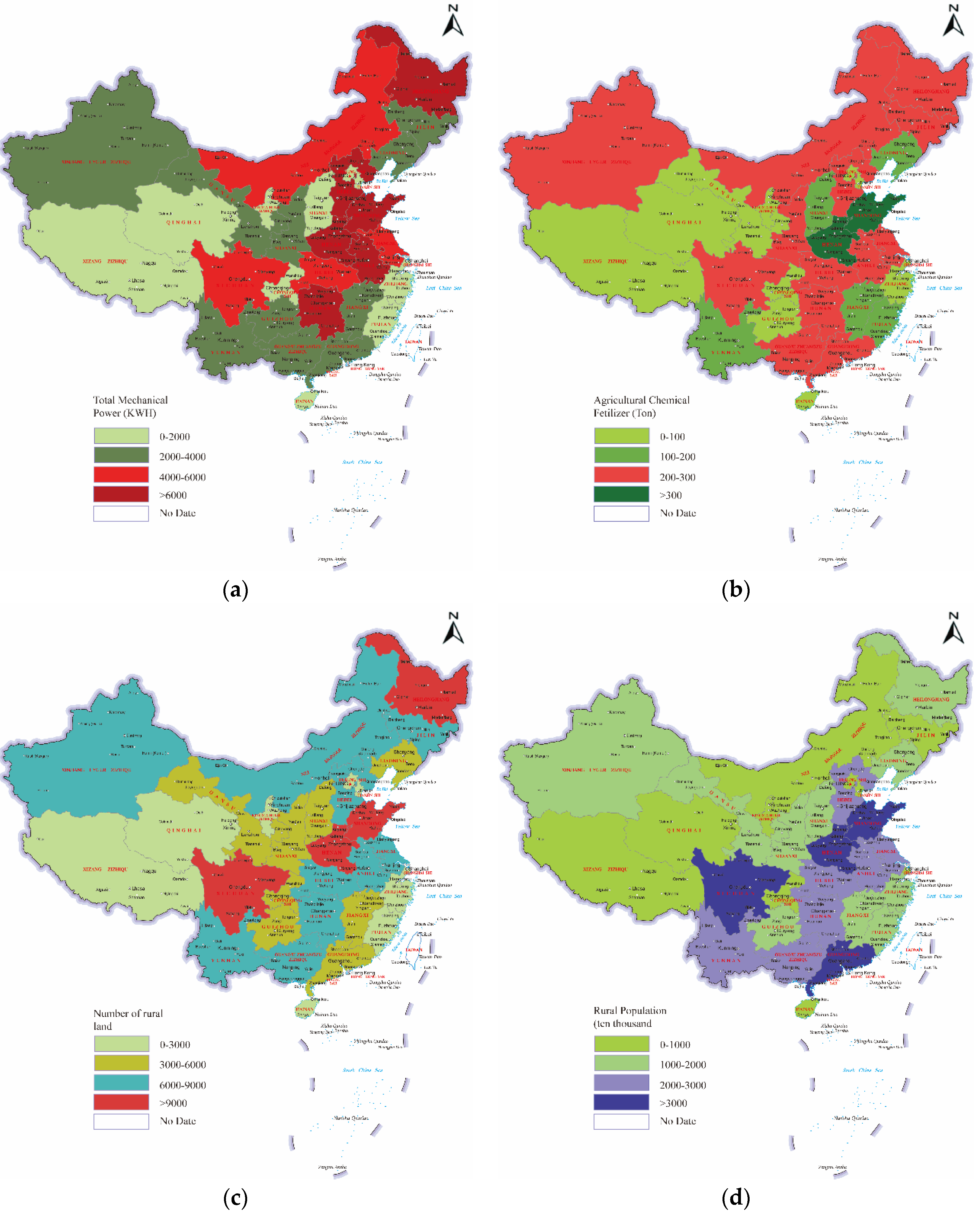
Through the spatialization analysis of the total power of agricultural machinery, fertilizer input, land input, and labor input, there was spatial heterogeneity between the inputs in different provinces. Specifically, in 2020 (
Figure 1), the provinces with a total mechanical power greater than 6000 KWH were mainly clustered in the main grain-producing areas, of which Heilongjiang, Henan, Shandong, and other provinces were representatives. The provinces with fertilizer inputs greater than 300 tons were Henan and Shandong; the provinces with larger agricultural land inputs were Henan, Shandong, Sichuan, and Heilongjiang; the provinces with large population inputs were Shandong, Henan, Guangxi, and Sichuan.
4. Conclusions
This paper takes the provincial panel data of China from 2001 to 2019 as the research unit, regards the narrow agriculture (planting industry) as the research object, uses the super efficiency SBM model to measure the inter-provincial agricultural ecological efficiency, and constructs the traditional and spatial Markov probability transfer matrix based on the time analysis of Kernel density estimation and the spatial correlation analysis of global Moran’s I index. Through the comparative analysis of the matrix, the temporal and spatial dynamic evolution characteristics of agricultural ecological efficiency are analyzed, and the influence of geospatial patterns on the temporal and spatial evolution of agricultural ecological efficiency is concluded. The main conclusions are as follows.
From the perspective of the difference in temporal evolution, the agricultural ecological efficiency of China based on line charts and Kernel density estimation shows a steady upward trend in fluctuations, and the volatility was mainly clustered around 2001–2019. From 2011 to 2019, there was still much space to improve agricultural ecological efficiency. The Kernel density estimation chart shows that the crest of the evolution of agricultural ecological efficiency in China has the distribution characteristics of a “double peak” from high to low, and the gap in wave crest height has narrowed. A “club convergence” pattern of “low agglomeration and high agglomeration” is gradually formed. This result is the same as Wang (2022) [
4].
From the perspective of spatial evolution, the results of the global Moran’s I index show that there was a significant positive correlation between the agricultural ecological efficiency of China and spatial distribution, and there was spatial dependence between interprovincial agricultural ecological efficiency. The traditional Markov probability transfer matrix presents that the overall trend of agricultural ecological efficiency shifting to a high level is significant, the evolution of agricultural ecological efficiency has the stability of maintaining the original state, and it is difficult to achieve leapfrog transfer. The probability of the type at both ends of the matrix remaining unchanged is the largest, and there is a possibility of “low agglomeration and high agglomeration”. The comparison between the spatial Markov probability transfer matrix and the traditional transfer matrix shows that, in addition to common characteristics, the geospatial pattern plays an important role in the spatial-temporal evolution of agricultural ecological efficiency and the spatial spillover effect is obvious. In different spatial contexts, the probability of the transfer of agricultural ecological efficiency types in different provinces has differences. If a province is adjacent to a province with a high agricultural ecological efficiency, the probability of upward transfer increases, while if it is adjacent to a province with low agricultural ecological efficiency, the probability of downward transfer increases. It means that provinces with high agricultural ecological efficiency enjoy positive spillover effects, while provinces with low agricultural ecological efficiency have negative spillover effects, so as to gradually form a “club convergence” of “high agglomeration, low agglomeration, high radiation and low inhibition” in the spatial pattern, which can echo the characteristics of time evolution. This result is the same as Guo (2020) [
14] and Liu (2020) [
15].
5. Discussion
Based on the super-efficiency SBM model and the spatial Markov probability transfer matrix, the spatial and temporal evolution characteristics of agricultural ecological efficiency in China are summarized as follows.
The super-efficient SBM model based on undesirable output can fully consider the impact of the resource environment on agricultural ecological efficiency and can further compare DMU with an efficiency of 1, but this paper does not discuss the various socio-economic factors that lead to the loss of agricultural ecological efficiency, because the loss of agricultural ecological efficiency is the result of the joint influence of various factors [
38]. Future research can consider structural changes, policy changes, technological changes, urbanization [
39], foreign direct investment (FDI), and other factors, as well as profoundly discussing the influencing factors of agricultural ecological efficiency loss.
The long-term evolution trend of China’s agricultural ecological efficiency shows that there is a huge potential for improvement in provinces with low agricultural ecological efficiency. The agricultural modernization of China is still facing the arduous task of resource conservation and environmental protection [
40]. In accordance with the requirements of green and low-carbon development, it is necessary to continue to deeply change the mode of agricultural economic development, pay attention to resource conservation and protection and the control of agricultural pollution emissions, learn from the experience of ecological agriculture management in neighboring provinces with high agricultural ecological efficiency, and reduce the provincial gap of agricultural ecological efficiency.


