Article

Carbon Emission Intensity Characteristics and Spatial Spillover Effects in Counties in Northeast China: Based on a Spatial Econometric Model

College of Earth Sciences, Jilin University, Changchun 130061, China
*
Author to whom correspondence should be addressed.
Land 2022, 11(5), 753; https://doi.org/10.3390/land11050753
Submission received: 29 April 2022 / Revised: 17 May 2022 / Accepted: 18 May 2022 / Published: 20 May 2022

Abstract

:
Under the “double carbon” target, it is important to reduce carbon emissions in each region. Using exploratory spatial data analysis (ESDA), the center of gravity method, and spatial econometric models, we analyzed the characteristics and spatial spillover effects of carbon emission intensity in counties in Northeast China from 2000 to 2020 and made recommendations to the government for more reasonable carbon reduction strategies in order to achieve sustainable development. The results were as follows: (1) Since 2000, the carbon emission intensity in Northeast China has increased after first declining, and the carbon emission intensity in the western and northern regions of Northeast China has increased faster than Northeast China’s average. (2) After 2000, the spatial aggregation of carbon emission intensity has improved in Northeast China. (3) Northeast China’s carbon emission intensity has a positive spatial spillover effect. Through the feedback mechanism, the growth in population size, the rise in economic development level, the level of industrialization as well as the rise in living standard, the land use structure dominated by arable land and construction land, and the increase in urbanization level in the region will cause the carbon emission intensity in the surrounding areas to increase. An increase in public expenditures leads to a decrease in carbon emission intensity in the adjacent area. (4) When the vegetation cover exceeds its threshold value, it can have a larger inhibitory influence on carbon emission intensity. To summarize, each county in Northeast China is a carbon emission reduction community, and policymakers must consider the spatial spillover effect of carbon emission intensity when developing policies.

1. Introduction

Global warming is a worldwide environmental issue. Global surface warming caused by humans is proportional to cumulative carbon emissions [1]. In response, the Chinese government clearly defined the “independent action target” at the 2015 Paris Climate Change Conference, namely, to achieve the peak of domestic carbon emissions around 2030 and strive to reach it as soon as possible, and to reduce carbon emission intensity by 60% to 65% in 2030 compared to 2005, to increase its independent national contribution to the issue. At the United Nations General Assembly’s 75th session in September 2020, the Chinese government expanded on its previous aims and ambitions by aiming for carbon neutrality by 2060.
Carbon intensity (the ratio of carbon emissions to GDP) can reflect a country’s or region’s level of carbon emissions in the process of economic development, and it’s also a key indicator for assessing regional carbon emissions performance [2,3]. Carbon emission intensity has been studied by several academics. The main focus is on the measurement of carbon emissions [4], the spatial correlation of carbon emission intensity [5], spatial and temporal evolution [6], spatial spillover effects [7], and influencing factors [8,9], etc. Agriculture [10], industry [11], service [12], tourism [13], and other industries are all involved.
In terms of research scale, existing research has primarily concentrated on national [14], provincial [15], and city levels [7], with only a few studies undertaken at the county level. According to the study’s findings, China’s carbon emission intensity is typically decreasing at both the province and city levels, and the spatial aggregation of carbon emission intensity appears to be optimized [7,16]. These studies, however, at both the provincial and municipal levels, look at the research region as a whole, which means it is homogeneous within it. In lower administrative regions, this is not necessarily appropriate for analyzing carbon intensity and formulating carbon reduction programs. This is because, even if it is the same city, the counties to which it belongs may be different. This is why county scales were used in this research. The formulation of policies to reduce carbon emissions requires an understanding of the elements that influence carbon intensity.
For the decomposition of influencing factors, researchers and policymakers have utilized a range of decomposition approaches, but no consensus exists on which method is the best. Other common methods such as LMDI (Logarithmic Mean Divisia Index) [17], STIRPAT [5], GWR (Geographically weighted regression model) [18], and the geographical detector method [19] are employed. For instance, using the LDMI model, Li et al. deconstructed the influencing variables of industrial carbon emissions in Northeast China, concluding that population, economy, and rate of industrialization are the pull factors for increasing industrial carbon emissions [20]. This study uses the STRIPAT model to investigate the influencing elements of carbon emission intensity because of its high scalability and validity. Several studies have revealed that population size [21], economic development level [5], industrialization level [22], public expenditure, and standard of living [23] all have a significant impact on carbon emission intensity. All of these variables are incorporated into the STRIPAT model. Furthermore, the level of urbanization is a significant contributing element. Based on Bai et al. [24], we utilize the nighttime light index to describe the level of urbanization at the county level. According to researchers [25], cultivated land and construction land are carbon sources. The more arable and construction land there is, the more human activities take place there and the more carbon emissions are produced. Vegetation’s photosynthesis can absorb a significant amount of carbon dioxide, making it one of nature’s most important carbon sinks. As a result, unlike earlier research, we took into account both the land use structure and the fractional vegetation cover to determine the amount of their impact on carbon intensity. In the Northeast China region, we hypothesize that land use structure contributes to carbon emission intensity while fractional vegetation cover suppresses it. To investigate these impacts, we employ the STIRPAT model and a spatial econometric model. Meanwhile, we focus on partial vegetation cover. We postulate that when fractional vegetation cover crosses a specific threshold, its suppressive effect becomes more prominent.
The northeast region of China has long been a heavy industrial base, with plentiful natural resources and high energy consumption, and it is also a critical area for reducing carbon emissions [26]. In this study, we examine the carbon emission intensity of Northeast China from the standpoint of counties. To begin with, we employ the gravity analysis approach to uncover the characteristics of carbon intensity in Northeast China since 2000. Then, we investigate the spatial correlation of carbon intensity in counties using exploratory spatial data analysis. Finally, we utilize a spatial econometric model to investigate the factors that influence county carbon emission intensity in Northeast China as well as the spatial spillover effects of each variable. A panel threshold model was used to investigate the threshold effects of fractional vegetation cover in the hopes of providing useful recommendations for achieving the “double carbon” target in Northeast China. The research design has three advantages. (1) The research scale has been decreased even further to the county level, which is more in line with the reality of spatial spillover effects. (2) The nighttime lighting index is used to determine the county’s level of urbanization, and it is more accessible than the complex evaluation. We also include land use structure and vegetation cover, which allows us to evaluate more influencing elements in terms of carbon sources and sinks. (3) We investigated the threshold value of vegetation, using a panel threshold model, which is useful in policymaking for quantifying some of the carbon reduction.

2. Materials and Methods

2.1. Study Area

Northeast China (Figure 1), consisting of Heilongjiang, Jilin, and Liaoning provinces, as well as Hulunbeier, Chifeng, Tongliao, and Xing’an League in the Inner Mongolia Autonomous Region, is the study area of this paper. Northeast China is located in the northeast of China and is a major industrial and agricultural center.
During the First Five-Year Plan period, Northeast China became the largest industrial base because it had a lot of natural resources and a unique history of growth [27]. Northeast China was formerly the cradle of Chinese industry, making significant contributions to the country’s economic development. Northeast China, however, saw a major economic decline in the 1990s due to resource depletion and environmental pollution. The revitalization of Northeast China’s old industrial bases, proposed in 2003, provided a strong opportunity for the region’s development. However, China’s previous economic development had relatively limited technology and equipment, and Northeast China’s economic recovery relied significantly on fossil energy use, which contributed to the release of large amounts of carbon dioxide [26,28]. Therefore, the selection of the Northeast China region for this study is typical and representative.
The study is on a county-by-county basis. To make the study feasible, the districts under the administration of each prefecture-level city were consolidated into one whole. Following the processing of missing data from several counties due to administrative division adjustments and missing data, there are 208 county study units left.

2.2. Variable Selection and Data Source

2.2.1. Variable Selection

Based on the previous work, this paper aims to analyze carbon emission intensity by using population size, economic development level, industrial structure, public expenditure, living standard, land use structure, nighttime light index, and fractional vegetation cover together as independent variables.
Among these independent variables, the land use structure data are the proportions of cropland and construction land to the administrative area. The nighttime light index, which uses the product of average light intensity and light area ratio to reflect the level of urbanization, is based on Bai et al. [24]. The average light intensity is calculated using the average DN value (DN value, that is, the pixel value of the night lighting raster data image element. Its value range is 0–63. The larger the value, the brighter the area) of the area’s nighttime light data. The light area ratio is the ratio of the area of the region with a DN value greater than zero to the area of the administrative region. One of nature’s most important carbon sinks is vegetation. Fractional vegetation cover is one of the influencing factors in this research. It is calculated by referring to the approach of the research method of Wei et al. [29].

2.2.2. Data Source

The carbon emission data in this paper is based on the research results of Chen et al. [30]. We utilized linear interpolation to extend the data to 2020 because this carbon emission data is only accessible for the years 2000–2017. The carbon emission intensity of the counties in Northeast China is calculated using the ratio of these carbon emissions to the GDP of the corresponding area. The study’s final carbon emission intensity data includes county carbon intensity data from 2000 to 2020, a period of 21 years. The China Statistical Yearbook, China City Statistical Yearbook, China Population, and Employment Statistical Yearbook, and statistical yearbooks of each city provide data on population size, economic development level, industrial structure, public expenditure, and living standards from 2000 to 2020. The land use data is obtained from the research results of Yang et al. [31]. The resolution is 30m and the time range is 2000–2020. The nighttime lighting data in this article comes from Zhang et al.’s [32] study results. The resolution is 1 km and the time range is 2000–2020. Fractional vegetation cover data is calculated using Landsat 7, with better quality images in the growing seasons (April–October) from 2000–2020 after de-clouding and other processing.

2.3. Research Methodology

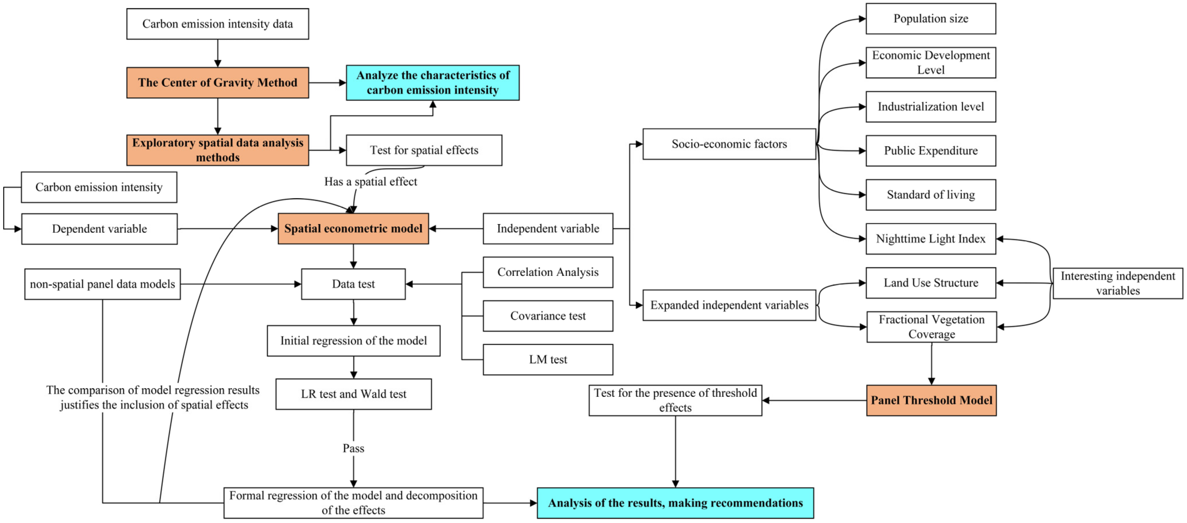
The research in this paper adheres to the following framework (Figure 2). We calculate the center of gravity of carbon emission intensity in Northeast China and analyze its characteristics. Exploratory spatial data analysis methods are used to examine the spatial correlation of carbon emission intensity data, and a spatial econometric model based on the STIRPAT model is introduced on the premise that it has spatial impacts. After a series of tests, the model’s final form is defined, the findings are assessed, and recommendations are given. We are more concerned with the nighttime light index, land use structure, and fractional vegetation cover when choosing independent variables. We also explored the threshold effect of the fraction of vegetation cover using a panel threshold model.

2.3.1. Exploratory Spatial Data Analysis Methods

Exploratory spatial data analysis methods (ESDA) are a set of approaches for characterization and visualization of geographical distributions, identifying atypical locations (spatial outliers), uncovering spatial connection patterns (spatial clusters), and so on [33]. It is one of the most commonly used models for analyzing spatial autocorrelation. Global spatial autocorrelation analysis and local spatial autocorrelation analysis are the two basic types of analysis. The global Moran’s I index is used to accomplish global spatial autocorrelation analysis. The global Moran’s I index is used to examine the spatial distribution of a worthy attribute of a spatial object throughout the whole research region, representing the general trend or spatial dependency of data grouped in the area. The formula for the computation is:
I = n i = 1 n j = 1 n W ( ( y i y ¯ ) ( y j y ¯ ) ) i = 1 n j = 1 n W i = 1 n ( y i y ¯ ) 2
In Equation (1), I is the global Moran’s I index, n is the number of study units, y i represents the carbon emission intensity of i county, and W represents the spatial weight matrix.
However, global spatial autocorrelation analysis assumes that the space is homogeneous and that the entire study region has only one spatial trend. For determining the spatial agglomeration of a single region, local spatial autocorrelation analysis can be used. The formula for the computation is:
L o c a l   M o r a n s   I = ( y i y t ¯ ) j = 1 n W ( y j y ¯ t ) i = 1 n ( y i y ¯ t ) 2
In Equation (2), y i represents the carbon emission intensity of i county and W represents the spatial weight matrix. The type of carbon emission intensity clustering among local surrounding regions in the counties of Northeast China can be analyzed using the Moran scatter diagram.
According to the first law of geography, all things are related to other things, but nearby things are more related than farther away ones. A spatial weight matrix is a type of matrix that describes the spatial relationship between things [4]. The influence of carbon emission intensity between nearby counties is measured in this article using the Queen type of geographic adjacency spatial weight matrix. The value of an element W i j in the spatial weight matrix is set as follows:
W i j = 1 , c i t y   i   a n d   j   s h a r e   c o m m o n   e d g e   o r   v e r t i c e s 0 , c i t y   i   a n d   j   h a v e   n o   c o m m o n   e d g e   o r   v e r t i c e s       o r   i = j

2.3.2. The Center of Gravity Method

The existence of a location in the region where the contrast of forces in all directions is generally balanced is referred to as the center of gravity in geography. We estimated the carbon emission intensity center of gravity in order to examine the characteristics of the change in carbon emission intensity in Northeast China since 2000. Quah [34], too, uses the center of gravity to highlight the shifting dynamics of the global economy. Its formula is as follows:
X = i = 1 n M X i i = 1 n M
Y = i = 1 n M Y i i = 1 n M
In Equations (4) and (5), X and Y represent the latitude and longitude of the center of gravity of carbon emission intensity in Northeast China, X i and Y i represent the coordinates of counties in Northeast China, M represents the carbon emission intensity.

2.3.3. Spatial Econometric Model

Dietz and Rosa [35] created the STIRPAT model, a stochastic version of the IPAT model, to find drivers with environmental impact in the empirical study [4]. The fundamental formula is as follows:
I i t = α P i t β A i t δ T i t λ e i t
In Equation (6), I represents environmental impact, P represents demographic factors, A represents economic factors, and T represents technological factors; i represents the region, t represents the year, α , β , δ and λ represents the coefficient, and e i t is the random error.
The STIRPAT model [36] has high extensibility and can determine the coefficients of each influencing element of carbon emission intensity. The model has already been utilized by some researchers [5,21] to investigate the factors that influence carbon emissions. The STIRPAT model’s logarithmic form can assist in avoiding some endogeneity issues while also making calculation easier. It is set as follows:
ln ( I i t ) = β ln ( P i t ) + δ ln ( A i t ) + λ ln ( T i t ) + a + e i t
where a represents the constant term and the rest is the same as in Equation (6).
The observed values of each variable in surrounding locations are correlated to some extent in our dataset. Any county’s carbon emission intensity is not independent, and it is always interacting with its surroundings. At the same time, the level of economic development in nearby regions is also related. There is a spatial effect, in other words. We investigate this issue by combining a spatial econometric model that can account for spatial impacts with the STIRPAT model. The spatial lag model (SLM), spatial error model (SEM), and spatial Durbin model (SDM) are the most common spatial econometric models. SLM and SEM are particular cases of SDM among them. Based on the suggestion in [37], we derive them from the general form of the spatial econometric model. The spatial econometric model’s general form is as follows:
φ i t = δ i = 1 n W i j φ i t + ε i t ln ( Y i t ) = ρ i = 1 n W i j ln ( Y i t ) + ln ( X k , i t ) β k + i = 1 n W i j ln ( X k , i t ) η k + μ i + λ t + φ i t
In Equation (7), Y i t denotes carbon emission intensity in counties i at year t , ρ , η and δ are the spatial autoregressive coefficients, X K , i t is the independent variable (Table 1), β is the coefficient of the independent variable, μ i and λ t are the spatial-specific effect and the time-specific effect, respectively, φ i t is the error term matrix, ε i t is the random error term, and W i j is the spatial weight matrix. Stata [38] and Matlab software are used to pick the models as well as carry out the modeling.
If η = δ = 0, there is a strong spatial dependence among the dependent variables, and the dependent variables in neighboring places affect the local dependent variables through a spatial transmission mechanism. This is called a spatial lag model (SLM). If η = ρ = 0 and δ ≠ 0, error terms in surrounding areas affect the local dependent variables through a spatial transmission mechanism. This is called a spatial error model (SEM). If ρ ≠ 0, η ≠ 0 and δ ≠ 0, changes in the dependent variable in a region are influenced not only by the independent variable in the region but also by changes in the independent and dependent variables in neighboring places, as well as the error term in the surrounding region. With spatial lags and errors, this is the most comprehensive spatial Durbin model (SDM) [39].
However, according to the results of James et al. [40], there are some mistakes in applying the coefficients calculated from the spatial Durbin model directly to explain the spatial spillover effects for the spatial lag term. The spatial Durbin model’s spatial lag coefficients and indirect effects are different. Due to the presence of feedback effects in the spatial Durbin model, the spatial lagged terms of the independent variables do not accurately reflect their spatial spillover effects. A partial differential is used to decompose it into direct and indirect effects. First, in matrix form, we write the equations of the spatial Durbin model generated from the previous equation.
Y t = ρ W Y t + X t β + W X t η + μ + λ t l n + φ t
where Y t is a vector of n × 1 dependent variables; X t is an n × k matrix of all independent variables; l n is an n × 1 matrix whose elements are all 1, and the remaining variables have the same meaning as above. At a given time t , the partial differential matrix of the dependent variable Y with regard to the k th independent variable can be expressed as:
[ Y X 1 k Y X n k ] = Y 1 X 1 k Y 1 X n k Y n X 1 k Y n X n k = ( I ρ W ) 1 β k w 12 η k w 1 n η k w 21 η k β k w 2 n η k w n 1 η k w n 2 η k β k
where the direct effect is the mean value on the main diagonal of the matrix at the right end. The indirect effect is the mean of the elements of the matrix at the right end other than on the main diagonal. The total effect is the sum of the direct and indirect effects.

2.3.4. Panel Threshold Model

To test our hypothesis that there may be a threshold effect between fractional vegetation cover and carbon emission intensity, we used a panel threshold model based on the STIRPAT model. This independent variable is known as the threshold variable, and when its values are in various ranges, the independent variables have different action relationships with the dependent variable. It is set up like this:
ln ( Y i t ) = β k ln ( X k , i t ) + α 1 ln ( F V C ) ( ln ( F V C ) λ ) + α 2 ln ( F V C ) ( ln ( F V C ) > λ ) + μ i + ε i t
where β k , α 1 and α 2 represent coefficients, X k , i t represents the remaining independent variables, λ represents the threshold value, μ i represents individual fixed effects, ε i t is the random error term.

3. Results

3.1. The Overall State of Carbon Emission Intensity in Northeast China’s Counties

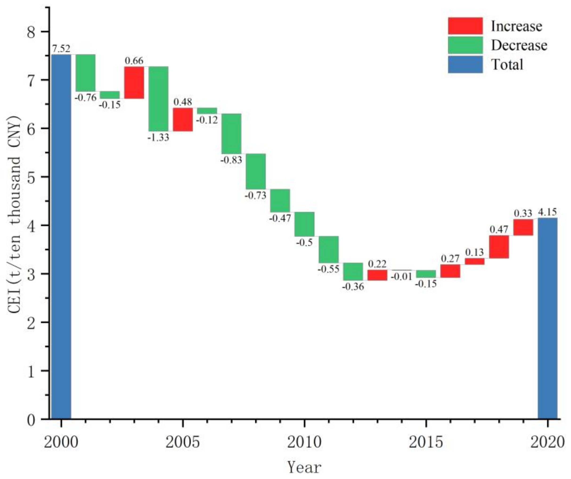
Overall, the intensity of carbon emissions in Northeast China has been falling and then increasing (Figure 3). Between 2000 and 2012, it fell by 61.97 percent, from 7.52 to 2.86 tons per ten thousand yuan, then rising between 2013 and 2020. The two years with the greatest year-on-year reductions were 2004 and 2007. They were 1.33 tons per 10,000 yuan and 0.83 tons per 10,000 yuan, respectively. With rises of 0.66 t/ten thousand yuan and 0.48 t/ten thousand yuan, respectively, 2003 and 2005 had the biggest year-on-year gains. Historical data reveals that the carbon emission intensity of Northeast China remains relatively high when compared to the carbon emission intensity of all Chinese counties [41], indicating that Northeast China still has a lot of room to cut carbon emissions.

3.2. Analysis of the Carbon Emission Intensity Center of Gravity Shift in Northeast China’s Counties

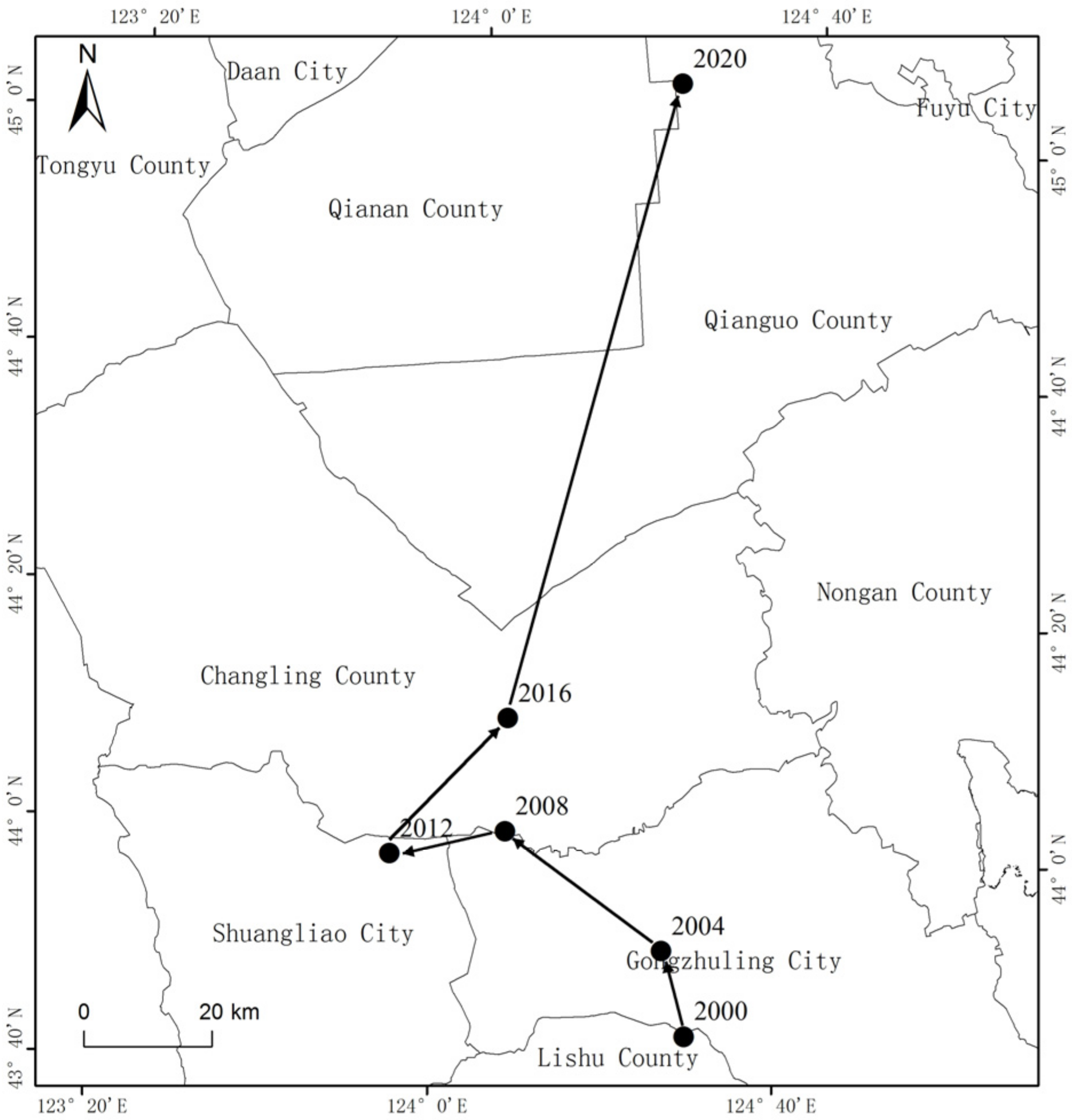
Using ArcGIS 10.2 software, the center of gravity of carbon emission intensity in the counties of Northeast China was investigated, and the findings are given in Figure 4. According to the dispersion of the center of gravity, the center of gravity of carbon emission intensity in Northeast China shifted between 123.8620°~124.4933°E and 43.7397°~45.0817°N, compared to the geometric center of Northeast China (125.0565°E, 44.4139°N). Since 2000, the center of gravity of carbon emission intensity in Northeast China has shown a trend of moving from south to north. It moves from Lishu County to the northwest to Gongzhuling City, then to the northwest toward Changling County, and finally to the north to Qianguo County. The carbon emission intensity in Northeast China gradually shifts to the northwest as well as to the north, indicating that the growth rate of carbon emission intensity in the western and northern regions of Northeast China is higher than the average level in Northeast China.

3.3. Carbon Emission Intensity in Northeast China: A Spatial Correlation Study

We combined the global Moran’s I index and the Local Moran’s I index to reflect the spatial correlation of carbon emission intensity in Northeast China. The global Moran’s I index of carbon emission intensity in counties in Northeast China is positive and passed the 1% significance test with positive spatial correlation, indicating that the spatial distribution of carbon emission intensity in counties in Northeast China has significant spatial aggregation characteristics and is not random, according to the findings (Table 2).
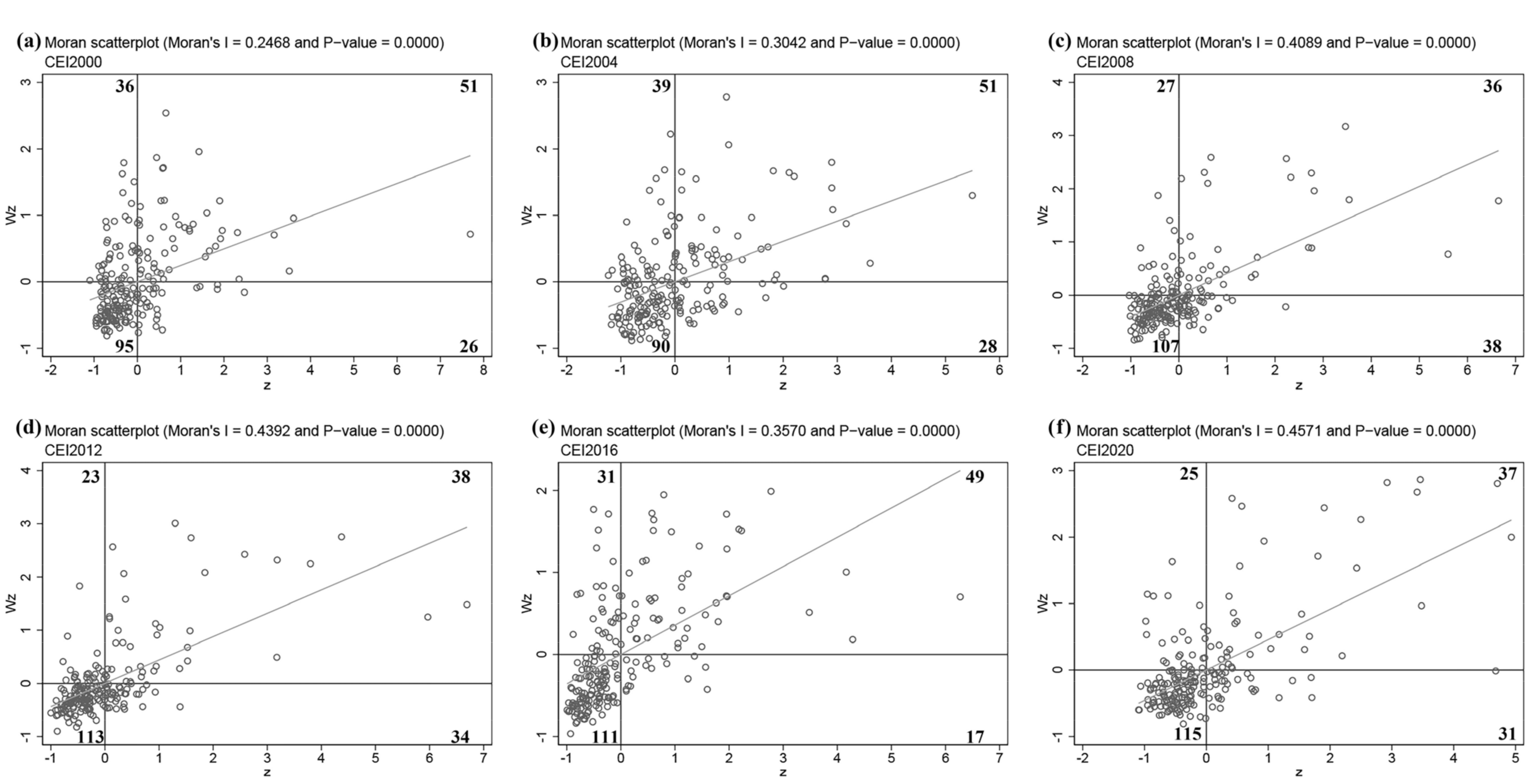
From a macroscopic perspective, global Moran’s I index can only show the overall spatial dependence characteristics of carbon emission intensity in the counties of Northeast China, namely, positive spatial correlations and aggregations, but the specific forms of aggregations should be shown using local spatial autocorrelation analysis. The local spatial autocorrelation analysis (Moran scatter plot (Figure 5); the numbers in the chart below show how many counties are in each quadrant) could illustrate the local spatial dependency features of each county. The results show that (1) the spatial and temporal distribution patterns of both agglomeration and divergence may be seen in the local autocorrelation of carbon emission intensity in counties in northeast China. However, counties in Northeast China have a high concentration of carbon emission intensity in the first and third quadrants, indicating that the carbon emission intensity distribution has strong spatial clustering features. During the research period, the number of counties in Northeast China that showed aggregation (high–high or low–low) surpassed 140, accounting for more than 67 percent, with the greatest number of 163 in 2014. The number of counties in the third quadrant (low–low aggregate) greatly outnumbers those in the high–high aggregate, suggesting the efficiency of industrial structure optimization and emission reduction in Northeast China; (2) After 2000, the spatial aggregation of carbon emission intensity in Northeast China’s counties exhibited a general optimization trend, with the number of counties with high–high aggregation somewhat reduced and those with low–low aggregation increasing.

3.4. A Study into the Spatial Spillover Effect of Carbon Emission Intensity in Northeast China

The results of the exploratory spatial data analysis (ESDA) approach demonstrate that the spatial distribution of carbon emission intensity in the counties of northeast China has considerable spatial clustering characteristics. Spatial econometric models are required to reflect the spatial impacts more completely and to investigate the spatial heterogeneity of the influencing variables of carbon emission intensity in various counties, as well as the spatial spillover effects.
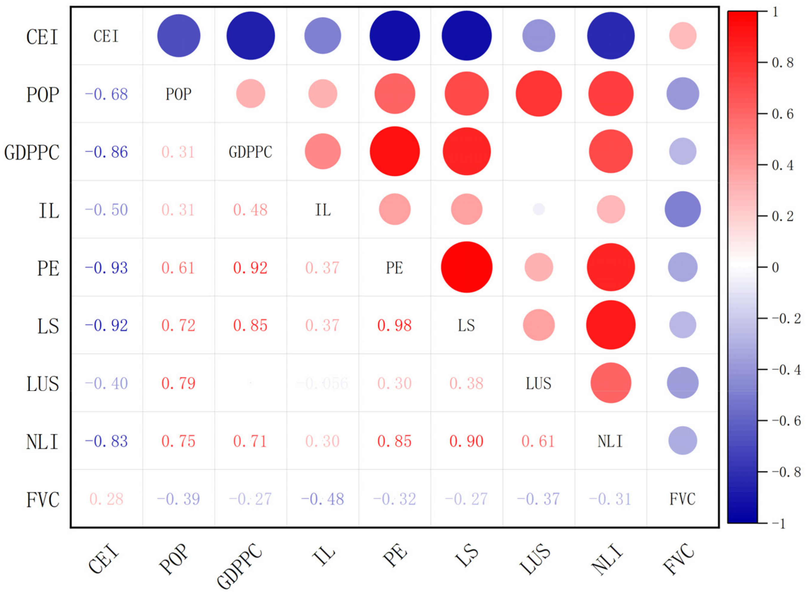
We ran a correlation analysis between the variables before running spatial regression (Figure 6). Positive correlations are shown by red circles, negative correlations are indicated by blue circles, and greater correlations are indicated by deeper hues and larger circles. This is performed to see whether there are any correlations between each independent variable and carbon emission intensity, which is required before spatial regression. The results reveal that each independent variable’s association with carbon intensity passed the 1% significance test, demonstrating that they are linked to carbon intensity. We then ran a colinearity test to see whether there was any serious collinearity between the variables, and the results revealed that the variance inflation factor had a mean value of 3.90 and a maximum value of 7.59, indicating that there was no serious colinearity.
We utilized Stata software to do a Hausman test to determine whether fixed or random effects should be employed, and the findings (124.33 with 8 degrees of freedom, p < 0.01) revealed that the original hypothesis of a random effect was rejected, and a fixed effect should be used instead. To figure out what kind of fixed effects existed in the data, we utilized a likelihood ratio test. At the 1% level, we found that the original hypothesis of joint insignificance of spatial fixed effects was rejected (1346.83, with 20 degrees of freedom, p < 0.01), as was the original hypothesis of joint insignificance of time-period fixed effects (11,378.64, with 207 degrees of freedom, p < 0.01). These test findings indicate that our data contains spatial and temporal dual fixed effects.
The estimation results for the non-spatial panel data models are reported in Table 3. The Lagrange multiplier test is Anselin’s [42] simple test diagnostic based on ordinary least squares (OLS) residuals to identify whether spatial lags or spatial error effects are present in our data. The results of the LM test are reported in the latter part of Table 3. Matlab software was used to generate the LM test.
According to the Lagrange multiplier test results, the p-values for the LM test for spatial errors as well as the robust LM test are less than 1%, rejecting the original hypothesis of no spatial errors and showing the presence of a spatial autocorrelation error term. Except for the spatial fixed effects model, which has a p-value of less than 10%, the LM test for spatial lags and the robust LM test have p-values of less than 1%, suggesting that the hypothesis of no spatial lag term is rejected. In conclusion, the spatial Durbin model (SDE) should be chosen for the regression of the model. Afterwards, the LR test and Wald test are used to determine whether the SDM will degenerate into SEM or SLM.
The results show that the initial hypothesis was rejected by both the LR and Wald tests (Table 4), demonstrating that SDE does not degenerate into SLM or SEM. As a result, for the regression, a spatial Durbin model with dual fixed effects in space and time-period should be used. The model’s regression results are reported in Table 4.
The coefficients of the independent variables in the spatial Durbin model are largely compatible with our theoretical assumptions, according to the regression results. Using the last column of Table 3 to compare with the coefficients of the spatial Durbin model, the coefficients of land use structure and nighttime light index were clearly exaggerated in the regressions without spatial effects. Only the spatial Durbin model with spatial effects passed the 1% significance test for fractional vegetation cover variables. This shows that including spatial effects in this research is reasonable.
The influence of each influencing factor on carbon emission intensity in Northeast China is revealed using a spatial Durbin model with the natural logarithm of carbon emission intensity as the dependent variable. The estimated coefficients of population size and economic development level are negative and much larger than those of other factors, passing the one-percent significance level test, indicating that population size and GDP per capita have a strong inhibitory effect on the change in carbon emission intensity. The estimated coefficient of industrialization level is positive and passes the one-percent significance level test, implying that failing to improve energy efficiency at higher levels of industrialization will increase carbon emission intensity. The negative coefficient of public expenditure passes the 1% significance level test, suggesting that a rise in local finance’s general budget expenditure has a dampening impact on the change in carbon emission intensity. The living standard coefficient is positive and passes the 1% significance level test, showing that an increase in living standard has a catalytic influence on changes in carbon emission intensity. The land use structure coefficient is positive and passes the 1% significance level test, demonstrating that the increase in farming and building land would increase carbon emission intensity. The nighttime light index coefficient is positive and passes the 1% significance level test, showing that the level of urbanization will enhance carbon emission intensity emission change. The fractional vegetation cover coefficient was negative and passed the 1% significance level test, showing that the variance in carbon emission intensity may be controlled by increasing the quantity of vegetation.
The direct effect is the magnitude of the effect of a county’s independent variable on carbon emission intensity, which includes the feedback effect; namely, the effect of a county’s independent variable on the carbon emission intensity of neighboring counties, which in turn affects the carbon emission intensity of that county. The sum of the spatial Durbin model coefficients and the feedback effect is the direct effect. The indirect effect, also known as the spatial spillover effect, is the impact of an adjacent county’s independent variable on the carbon emission intensity of this county. The total effect is the sum of the direct and indirect effects of an independent variable on the carbon emission intensity of all counties, given as the average effect of an independent variable on the carbon emission intensity of all counties. The findings of the effect decomposition are shown in Table 5.
The direct effects of population size and economic development level are negative, and the indirect effects are positive. It shows that while local carbon emission intensity is suppressed by population size and economic development, there is a strong positive spatial spillover effect that promotes carbon emission intensity increases in neighboring counties. Population growth has contributed to increased consumption of non-clean energy, building energy, and other forms of energy, resulting in increased CO2 emissions. However, population growth has also continued to inject new vitality into economic development and technological innovation, resulting in a decrease in carbon emission intensity. The negative direct effect of economic development implies that the good impact of economic growth overcomes the rise in CO2 emissions it causes, implying that a high rate of quality economic development is always a key influencing factor for green and low-carbon social development. However, as the region’s population and economy grow, it will attract population and economic migration from surrounding areas, resulting in inefficient resource use in the surrounding counties and thus increasing carbon emission intensity.
The level of industrialization has both direct and indirect positive effects. This shows that the accelerated speed of industrialization and the resources are not all being used rationally, resulting in irrational energy usage in the surrounding counties, which has a negative influence on carbon emissions in the surrounding counties, thereby increasing carbon emissions intensity.
Public expenditure has both direct and indirect negative effects. It indicates that the government’s investment in infrastructures such as roads and bridges, social services, and scientific research has, to some extent, promoted the rational use of the region’s resources and stimulated economic development and that the rational use of resources has caused carbon emissions to grow at a slower rate than the economy, resulting in a reduction in the region’s carbon emission intensity. Simultaneously, the flow of resources attracts the spatial migration of economic activities from nearby areas, resulting in more efficient use of resources and a commensurate reduction in carbon emission intensity.
The direct and indirect effects of the living standard were both positive, passing the 1% significance level test. It demonstrates that rising living standard has boosted consumer carbon emissions, owing to the market’s creation of a regional draw. Some manufacturing and service industries from neighboring regions will relocate to the region, while more manufacturing industries from neighboring regions will increase production to meet their own demand, resulting in unreasonable resource use and an increase in carbon emission intensity in the region and neighboring regions.
Land use structure had both direct and indirect positive and significant effects. This shows that increasing the area of tilled land and construction land can result in an increase in carbon emission intensity, either directly or indirectly. As a result, stringent land and space use regulations are required, with the present arable land acreage and quality being constant. Limit the conversion of arable land to construction land, keep the overall amount of construction land under control, and keep the total amount of construction land steady or decreasing.
The nighttime lighting index has both direct and indirect positive and significant effects. The nighttime lighting index might be a reliable predictor of overall urbanization levels [24]. This means that, as a result of urbanization, there will be a phenomenon of population and industrial agglomeration that will cause irrational resource use to some extent, resulting in an increase in carbon emission intensity in the region, and such a phenomenon will also affect the change in carbon emission intensity in neighboring regions.
Fractional vegetation cover had a negative direct effect and had no significant indirect effect. It means that the vegetation in this area exclusively helps to reduce carbon emission intensity in this area and has no effect on carbon emission intensity in nearby places. The vegetation’s spatial spillover effect was not significant. In addition, according to Wang et al. [43], we used Stata software to run a panel threshold model for fractional vegetation cover. The results revealed that fractional vegetation cover had a single threshold effect (p < 0.01), with a threshold value of −0.7662. It had a coefficient of −0.0531 when the fractional vegetation cover was less than or equal to −0.7662 (FVC less than or equal to 46.48 percent). It had a coefficient of −0.1294 when the fractional vegetation cover was greater than −0.7662 (FVC greater than 46.48 percent). This finding suggests that when the county’s vegetation cover is larger than 46.48 percent, the factor’s inhibitory effect on carbon emission intensity is increased by more than twofold.

4. Discussion

4.1. Comparative Analysis of the Results

Previous studies have looked at population size, economic development level, industrial structure, living standard, and public expenditure as independent variables of carbon emission intensity, with similar results [7,23,44]. Carbon emission intensity is suppressed by population size, economic development, and government expenditures, whereas carbon emission intensity is promoted by industrialization and living standard. All of the aforementioned parameters have a positive spatial spillover impact on the intensity of carbon emissions. The positive direct and indirect impacts of the nighttime lighting index are also as expected. However, unlike earlier research, we show that public expenditure has a large negative spatial spillover effect on carbon emission intensity. This might be due to the fact that government expenditure is driven by the public interest, which is more justifiable for energy usage. This might potentially be a viable proposal for lowering carbon emissions.
Chen et al. [30] obtained the carbon emission statistics of the county in this research by downscaling the province’s energy carbon emissions. Carbon emissions from various fossil fuels, such as raw coal and gasoline, are included in the statistics. To put it another way, it is energy-related carbon emissions. Because land use carries a substantial quantity of human production and living activities, we believe that land use (arable land and building land are considered in this research) has an impact on carbon emission intensity. Other than that, cropland and building land have been recognized as the main carbon sources in several studies [25,45]. As a result, we included land use structure (the ratio of cultivated and built land) as a factor that influences carbon emission intensity. The results show that there is a contributing influence of land use structure on carbon emission intensity as well as a spatial spillover effect, i.e., a contributing effect that also exists in the surrounding regions, which helps us make policies, which is consistent with our hypothesis.
Vegetation can absorb a considerable quantity of carbon dioxide through photosynthesis, making it an important carbon sink in nature. As a result, one of the determining elements is vegetation cover. The findings support our hypothesis that plant cover has a considerable inhibitory influence on carbon intensity. However, the conclusion that interests us is that vegetation cover has no spatial spillover effect, i.e., vegetation in our region has no influence on carbon intensity in the adjacent areas. As a result, rather than depending on the neighboring areas, regions with poor vegetation cover must grow a lot of vegetation in their own regions to absorb carbon emissions. In the meantime, we applied a panel threshold model to it. The findings demonstrate that when plant cover exceeds 46.48 percent, carbon intensity is inhibited by more than twice as much as previously. This enlightens us to concentrate on greening for counties that fall short of this standard.

4.2. Policy Implications

For the future growth of Northeast China, the following suggestions are offered:
(1)
Attaching great importance to the spatial correlation of carbon emission intensity and spatial spillover effects, creating carbon-cutting policies tailored to the needs of each location. As a carbon reduction community, to jointly accomplish the “double carbon” goal, all regions should work together to design carbon reduction policies and embrace a collaborative governance model of integrated planning, resource and information sharing, and industrial integration and development. Locations where carbon emission intensity is relatively high, and agglomeration occurs would drive the carbon emission intensity of their surrounding areas to increase as well. This necessitates an increase in public finance spending, the gradual reduction of coal-based high-consumption, high-emission development methods, industrial transformation and upgrading, and the maintenance of a high-quality level of economic development. Lower carbon-intensity regions should continue to use their spatial spillover effects to encourage nearby regions to pursue low-carbon green growth.
(2)
Determine the major directions for designing carbon reduction programs by grasping the dominant factors of high carbon emission intensity. The role of population size and level of economic development in curbing carbon emission intensity is highly valued. The population decrease in the northeast is alarming, and governments should take proactive measures to address it. They should improve social security policies and address employment issues, as well as change the industrial structure, elevate the status of tertiary industry in economic development, and capitalize on the “Belt and Road” development opportunity to resuscitate Northeast China’s traditional industrial bases.
(3)
Insist in land and space use regulation system. Keep the present arable land acreage and quality constant. Limit the conversion of arable land to construction land, keep the overall amount of construction land under control, and keep the total amount of construction land steady or decreasing.
(4)
Continue to focus on afforestation and urban greening to maintain a high level of vegetation cover and stabilize vegetation’s ability to sequester and reduce carbon. Greening activities should be prioritized in counties with poor vegetation cover, such as Tumen City and Yushu City. Northeast China should continue to excavate the potential of forest carbon sinks and engage in carbon market activities.

4.3. Uncertainties and Prospects

On the one hand, due to the partial absence of raw data on carbon emissions in some counties (including the absence of carbon emission data in some counties and the fact that data for the most recent years are not available), this paper may have an impact on the spatial correlation of carbon emission intensity in the Northeast China region as a whole, which may be analyzed for the entire region in the future when the data is expanded. On the other hand, because of administrative changes and a lack of data, county data indicators and data quality are still in need of improvement. Therefore, more optimal data can be used in the future to examine the influencing variables of carbon emission intensity in Northeast China counties.
In addition to that, the impact on the carbon emission intensity of the entire region can be assessed in the future in terms of the kind and volume of vegetation with various carbon sequestration levels. Meanwhile, more influencing factors in terms of carbon sources (e.g., energy consumption, which is not counted or data is difficult to obtain in Chinese counties) and carbon sinks (e.g., area of ecological land, etc.) could be added in the future to analyze the carbon emission intensity of counties in Northeast China.

5. Conclusions

The research timeframe for this research is 2000–2020. We investigated the characteristics of carbon emission intensity as well as spatial correlation in the counties of Northeast China using exploratory spatial analysis methods and the center of gravity approach. We investigated the influence elements of carbon emission intensity and the spatial spillover effect using a spatial econometric model, as well as the threshold effect of vegetation cover using a panel threshold model. We intend to offer practical suggestions for reducing carbon emissions in Northeast China. The following are the conclusions:
(1)
Since 2000, the carbon emission intensity in the Northeast has increased after first declining, and the growth rate of carbon emission intensity in the western and northern regions of Northeast China is higher than the average level in Northeast China. Carbon emission intensity has a spatial correlation in northeast China. Since 2000, the spatial aggregation of carbon emission intensity has improved.
(2)
The results of the spatial econometric model show that in the counties of Northeast China, population size, economic development level, public expenditure, and fractional vegetation cover have a suppressive effect on carbon emission intensity. When the vegetation cover exceeds its threshold value, it can have a larger inhibitory influence on carbon emission intensity. The level of industrialization, living standard, land use structure dominated by arable land and construction land, and urbanization level all promote the increase of carbon emission intensity. The population size and level of economic development are significant driving forces among them.
(3)
Northeast China’s carbon emission intensity has a positive spatial spillover effect. Through the feedback mechanism, the increase in population size, the rise in economic development level, the level of industrialization as well as the improvement of living standard, the land use structure dominated by arable land and construction land, and the increase in urbanization level in the region will increase the carbon emission intensity in the surrounding areas. An increase in public expenditures leads to a decrease in carbon emission intensity in the surrounding area. The change in vegetation cover in this area does not affect the surrounding areas.

Author Contributions

Conceptualization, S.L. and Y.L.; methodology, Z.G. and X.C.; software, Z.G. and X.C.; validation, S.L.; formal analysis, Z.G., X.C. and S.L.; investigation, Z.G.; resources, Z.G. and X.C.; data curation, Z.G. and X.C.; writing—original draft preparation, Z.G.; writing—review and editing, S.L. and Y.L.; visualization, Z.G.; supervision, S.L.; project administration, S.L.; funding acquisition, S.L. and Y.L.; All authors have read and agreed to the published version of the manuscript.

Funding

This work was supported by the National Natural Science Foundation of China (Grant No. 42177447), the Science and Technology Development Plan Project of Jilin Province (Grant No. 20210203010SF), and the Natural Science Foundation of Jilin Province, China (Grant No. 20210101395JC).

Institutional Review Board Statement

Not applicable.

Informed Consent Statement

Not applicable.

Data Availability Statement

Not applicable.

Acknowledgments

The nighttime lighting data is provided by the National Tibetan Plateau Data Center (http://data.tpdc.ac.cn) (accessed on 3 March 2022). Many thanks to the reviewers and the editors for their insightful and constructive comments and suggestions.

Conflicts of Interest

The authors declare no conflict of interest.

References

  1. Bronselaer, B.; Zanna, L. Heat and carbon coupling reveals ocean warming due to circulation changes. Nature 2020, 584, 227–233. [Google Scholar] [CrossRef] [PubMed]
  2. Chen, H.; Qi, S.Z.; Tan, X.J. Decomposition and prediction of China’s carbon emission intensity towards carbon neutrality: From perspectives of national, regional and sectoral level. Sci Total Environ. 2022, 825, 14. [Google Scholar] [CrossRef] [PubMed]
  3. Dong, F.; Yu, B.L.; Hadachin, T.; Dai, Y.J.; Wang, Y.; Zhang, S.N.; Long, R.Y. Drivers of carbon emission intensity change in China. Resour. Conserv. Recycl. 2018, 129, 187–201. [Google Scholar] [CrossRef]
  4. Lv, T.; Hu, H.; Zhang, X.M.; Xie, H.L.; Wang, L.; Fu, S.F. Spatial spillover effects of urbanization on carbon emissions in the Yangtze River Delta urban agglomeration, China. Environ. Sci. Pollut. Res. 2022, 29, 33920–33934. [Google Scholar] [CrossRef]
  5. Wang, Y.; Zheng, Y. Spatial effects of carbon emission intensity and regional development in China. Environ. Sci. Pollut. Res. 2021, 28, 14131–14143. [Google Scholar] [CrossRef]
  6. Zeyang, C.; Jingang, Y.; Jian, S. An analysis of regional carbon intensity space—Time evolution and its influence factors in China. Sci. Technol. Manag. Res. 2017, 37, 260–266. [Google Scholar]
  7. Wang, S.; Huang, Y.; Zhou, Y. Spatial spillover effect and driving forces of carbon emission intensity at the city level in China. J. Geogr. Sci. 2019, 29, 231–252. [Google Scholar] [CrossRef] [Green Version]
  8. Song, M.; Wu, J.; Song, M.; Zhang, L.; Zhu, Y. Spatiotemporal regularity and spillover effects of carbon emission intensity in China’s Bohai Economic Rim. Sci. Total Environ. 2020, 740, 140184. [Google Scholar] [CrossRef]
  9. Bhattacharyya, S.C.; Matsumura, W. Changes in the GHG emission intensity in EU-15: Lessons from a decomposition analysis. Energy 2010, 35, 3315–3322. [Google Scholar] [CrossRef]
  10. Pang, J.X.; Li, H.J.; Lu, C.P.; Lu, C.Y.; Chen, X.P. Regional differences and dynamic evolution of carbon emission intensity of agriculture production in China. Int. J. Environ. Res. Public Health 2020, 17, 7541. [Google Scholar] [CrossRef]
  11. Yu, S.W.; Hu, X.; Fan, J.L.; Cheng, J.H. Convergence of carbon emissions intensity across Chinese industrial sectors. J. Clean. Prod. 2018, 194, 179–192. [Google Scholar] [CrossRef]
  12. Yu, J.H.; Yu, Y.; Jiang, T.Y. Structural factors influencing energy carbon emissions in China’s service industry: An input-output perspective. Environ. Sci. Pollut. Res. 2022. [Google Scholar] [CrossRef] [PubMed]
  13. Tong, Y.; Zhang, R.; He, B. The carbon emission reduction effect of tourism economy and its formation mechanism: An empirical study of China’s 92 tourism-dependent cities. Int. J. Environ. Res. Public Health 2022, 19, 1824. [Google Scholar] [CrossRef] [PubMed]
  14. Xianzhao, L.; Zhangchun, G.; Yong, Z.; Dongshui, Z.; Jinning, X.; Yan, S.; Zhiqiang, W. Spatial dependence pattern of carbon emission intensity in China’s provinces and spatial heterogeneity of its influencing factors. Sci. Geogr. Sin. 2018, 38, 681–690. [Google Scholar]
  15. Zheng, Y.M.; Lv, Q.; Wang, Y.D. Economic development, technological progress, and provincial carbon emissions intensity: Empirical research based on the threshold panel model. Appl. Econ. 2021, 54, 3495–3504. [Google Scholar] [CrossRef]
  16. Zhou, Y.Y.; Xu, Y.R.; Liu, C.Z.; Fang, Z.Q.; Guo, J.Y. Spatial effects of technological progress and financial support on China’s provincial carbon emissions. Int. J. Environ. Res. Public Health 2019, 16, 1743. [Google Scholar] [CrossRef] [Green Version]
  17. Li, H.; Wu, L. Analysis of Hubei province industry’s carbon emissions based on the LMDI. In Proceedings of the 2nd International Conference on Renewable Energy and Environmental Technology (REET), Dalian, China, 19–20 August 2014; pp. 1865–1868. [Google Scholar]
  18. Li, W.; Sun, W.; Li, G.M.; Jin, B.H.; Wu, W.; Cui, P.F.; Zhao, G.H. Transmission mechanism between energy prices and carbon emissions using geographically weighted regression. Energy Policy 2018, 115, 434–442. [Google Scholar] [CrossRef]
  19. Zhang, W.; Feng, P.F. Differentiation research of CO2 emissions from energy consumption and their influencing mechanism on the industrial enterprises above designated size in Chinese industrial cities: Based on geographical detector method. Nat. Hazards 2020, 102, 645–658. [Google Scholar] [CrossRef] [Green Version]
  20. Li, S.P.; Wang, Q.; Meng, Y. Analysis on the status and influencing factors of industrial carbon emissions in Northeast China. In Proceedings of the 3rd International Conference on Energy, Environment and Sustainable Development (EESD 2013), Shanghai, China, 12–13 November 2013; pp. 866–869. [Google Scholar]
  21. Gong, W.-F.; Fan, Z.-Y.; Wang, C.-H.; Wang, L.-P.; Li, W.-W. Spatial spillover effect of carbon emissions and its influencing factors in the Yellow River basin. Sustainability 2022, 14, 3608. [Google Scholar] [CrossRef]
  22. Qin, J.C.; Tao, H.; Zhan, M.J.; Munir, Q.; Brindha, K.; Mu, G.J. Scenario analysis of carbon emissions in the energy base, Xinjiang autonomous region, China. Sustainability 2019, 11, 4220. [Google Scholar] [CrossRef] [Green Version]
  23. Huibin, M.; Shaojian, W. Spatio-temporal evolution and spatial effect mechanism of carbon emission at county level in the Yellow River basin. Sci. Geogr. Sin. 2021, 41, 1324–1335. [Google Scholar]
  24. Heting, B.; Mingguo, M.; Ran, Y.; Kangning, L.; Chuhan, J. Evaluation of urban expansion in Chongqing city based on the nighttime light data. Remote Sens. Technol. Appl. 2019, 34, 216–224. [Google Scholar]
  25. Lin, Q.W.; Zhang, L.; Qiu, B.K.; Zhao, Y.; Wei, C. Spatiotemporal analysis of land use patterns on carbon emissions in China. Land 2021, 10, 141. [Google Scholar] [CrossRef]
  26. Liu, X.Y.; Duan, Z.Y.; Shan, Y.L.; Duan, H.Y.; Wang, S.; Song, J.N.; Wang, X.E. Low-carbon developments in Northeast China: Evidence from cities. Appl. Energy 2019, 236, 1019–1033. [Google Scholar] [CrossRef] [Green Version]
  27. Zhang, P.Y. Revitalizing old industrial base of Northeast China: Process, policy and challenge. Chin. Geogr. Sci. 2008, 18, 109–118. [Google Scholar] [CrossRef]
  28. Liu, S.B. Energy consumption and structural reformation in Chinese northeast old industrial base. In Proceedings of the International Conference on Renewable Energy and Environmental Technology (REET 2013), Jilin, China, 21–22 September 2013; pp. 4281–4284. [Google Scholar]
  29. Wei, X.D.; Wang, S.N.; Wang, Y.K. Spatial and temporal change of fractional vegetation cover in North-western China from 2000 to 2010. Geol. J. 2018, 53, 427–434. [Google Scholar] [CrossRef] [Green Version]
  30. Chen, J.; Gao, M.; Cheng, S.; Hou, W.; Song, M.; Liu, X.; Liu, Y.; Shan, Y. County-level CO2 emissions and sequestration in China during 1997–2017. Sci. Data 2020, 7, 391. [Google Scholar] [CrossRef] [PubMed]
  31. Yang, J.; Huang, X. The 30 m annual land cover dataset and its dynamics in China from 1990 to 2019. Earth Syst. Sci. Data 2021, 13, 3907–3925. [Google Scholar] [CrossRef]
  32. Lixian, Z.; Zhehao, R.; Bin, C.; Peng, G.; Haohuan, F.; Bing, X. A Prolonged Artificial Nighttime-Light Dataset of China (1984–2020); National Tibetan Plateau Data Center: Beijing, China, 2021. [Google Scholar] [CrossRef]
  33. Anselin, L. Interactive techniques and exploratory spatial data analysis. Geogr. Inf. Syst. Princ. Tech. Manag. Appl. 1999, 47, 415–421. [Google Scholar] [CrossRef]
  34. Quah, D. The global economy’s shifting centre of gravity. Glob. Policy 2011, 2, 3–9. [Google Scholar] [CrossRef]
  35. Dietz, T.; Rosa, E.A. Effects of population and affluence on CO2 emissions. Proc. Natl. Acad. Sci. USA 1997, 94, 175–179. [Google Scholar] [CrossRef] [PubMed] [Green Version]
  36. Li, W.; Du, L. Assessment framework of provincial carbon emission peak prediction in China: An empirical analysis of Hebei province. Pol. J. Environ. Stud. 2019, 28, 3753–3765. [Google Scholar] [CrossRef]
  37. Elhorst, J.P. Matlab software for spatial panels. Int. Reg. Sci. Rev. 2014, 37, 389–405. [Google Scholar] [CrossRef] [Green Version]
  38. Belotti, F.; Hughes, G.; Mortari, A.P. Spatial panel-data models using Stata. Stata J. 2017, 17, 139–180. [Google Scholar] [CrossRef] [Green Version]
  39. Repkine, A.; Min, D. Foreign-funded enterprises and pollution halo hypothesis: A spatial econometric analysis of thirty Chinese regions. Sustainability 2020, 12, 5048. [Google Scholar] [CrossRef]
  40. James, L.; Robert, K.P. Introduction to Spatial Econometrics; CRC Press: Boca Raton, FL, USA, 2009. [Google Scholar]
  41. Wenmeng, Y.; Tingting, Z.; Dajun, S. County-level spatial pattern and influencing factors evolution of carbon emission intensity in China: A random forest model analysis. China Environ. Sci. 2022, 1–10. Available online: https://kns.cnki.net/kcms/detail/11.2201.X.20220219.1311.002.html (accessed on 3 March 2022).
  42. Anselin, L.; Bera, A.K.; Florax, R.; Yoon, M.J. Simple diagnostic tests for spatial dependence. Reg. Sci. Urban Econ. 1996, 26, 77–104. [Google Scholar] [CrossRef]
  43. Wang, Q.Y. Fixed-effect panel threshold model using Stata. Stata J. 2015, 15, 121–134. [Google Scholar] [CrossRef] [Green Version]
  44. Han, X.; Cao, T.; Sun, T. Analysis on the variation rule and influencing factors of energy consumption carbon emission intensity in China’s urbanization construction. J. Clean. Prod. 2019, 238, 117958. [Google Scholar] [CrossRef]
  45. Zhao, R.Q.; Huang, X.J.; Liu, Y.; Zhong, T.Y.; Ding, M.L.; Chuai, X.W. Carbon emission of regional land use and its decomposition analysis: Case study of Nanjing city, China. Chin. Geogr. Sci. 2015, 25, 198–212. [Google Scholar] [CrossRef]
Figure 1. The spatial location of the study area.
Land 11 00753 g001
Figure 2. The research framework of this study. The orange represents the research methodology and the blue filled represents the part where the main conclusions were obtained.
Land 11 00753 g002
Figure 3. Changes in the average carbon emission intensity of counties in Northeast China.
Land 11 00753 g003
Figure 4. Analysis of the center of gravity shift of carbon emission intensity in Northeast China.
Land 11 00753 g004
Figure 5. Moran scatter plot of carbon emission intensity at the county level in Northeast China. (a) 2000; (b) 2004; (c) 2008; (d) 2012; (e) 2016; (f) 2020.
Land 11 00753 g005
Figure 6. Results of the correlation test.
Land 11 00753 g006
Table 1. Variable definitions.
VariableAbbreviationNameDefinitionNumber of Observations
Dependent variableCEICarbon emission intensityCO2 emissions/GDP (t/ten thousand CNY)4368
Independent variablesPOPPopulation sizePopulation (ten thousand people)4368
GDPPCEconomic Development LevelGDP/Population (ten thousand CNY/per person)4368
ILIndustrialization levelValue added by the secondary industry/GDP4368
PEPublic ExpenditureExpenditures from the general public budget of local governments (ten thousand CNY)4368
LSStandard of livingSavings account balance for residents (ten thousand CNY)4368
LUSLand Use StructurePercentage of cropland and construction land4368
NLINighttime Light IndexThe product of average light intensity and light area ratio4368
FVCFractional Vegetation CoveragePercentage of vegetation area4368
Table 2. Moran’s I index test results from 2000 to 2020.
YearIZP
20000.2468 ***5.92710.0000
20010.2936 ***6.78960.0000
20020.3018 ***7.00660.0000
20030.2334 ***5.74860.0000
20040.3042 ***7.05680.0000
20050.3298 ***7.72910.0000
20060.3597 ***8.43080.0000
20070.3698 ***8.77360.0000
20080.4089 ***9.67350.0000
20090.4258 ***10.04420.0000
20100.4586 ***10.86320.0000
20110.4489 ***10.77450.0000
20120.4392 ***10.46010.0000
20130.3869 ***9.12000.0000
20140.3844 ***9.05990.0000
20150.4238 ***9.95710.0000
20160.357 ***8.35540.0000
20170.4218 ***9.79920.0000
20180.4786 ***11.06020.0000
20190.4363 ***10.14790.0000
20200.4571 ***10.61990.0000
Note: *** means significant within 1%.
Table 3. Estimation results of non-spatial panel data models.
Pooled OLSSpatial Fixed
Effects
Time-Period
Fixed Effects
Spatial and Time-
Period Fixed Effect
ln (POP)−0.4247 ***−0.8335 ***−0.4246 ***−0.8449 ***
(0.0167)(0.0178)(0.0195)(0.0159)
ln (GDPPC)−0.6870 ***−0.8636 ***−0.6623 ***−0.8987 ***
(0.0162)(0.0083)(0.0165)(0.0079)
ln (IL)−0.01840.0154 **0.01020.0673 ***
(0.0146)(0.0071)(0.0156)(0.0068)
ln (PE)0.0218 *0.0496 ***0.0415 **−0.0632 ***
(0.0131)(0.0071)(0.0183)(0.0078)
ln (LS)0.0838 ***0.1399 ***0.0603 ***0.0839 ***
(0.0129)(0.0067)(0.0144)(0.0075)
ln (LUS)−0.2016 ***0.1092 **−0.1926 ***0.2166 ***
(0.0100)(0.0349)(0.0105)(0.0309)
ln (NLI)0.1421 ***0.1749 ***0.1406 ***0.1668 ***
(0.0062)(0.0031)(0.0068)(0.0032)
ln (FVC)−0.3295 ***−0.0574 ***−0.2865 ***0.0010
(0.0267)(0.0155)(0.0277)(0.0139)
constant0.9209 ***2.2196 ***1.0599 ***4.5484 ***
(0.1173)(0.1089)(0.1470)(0.1392)
Adjusted. R20.5960.9580.6030.969
No. Obs.4368436843684368
LM Spatial Lag1080.5710 ***159.0936 ***41.2029 ***58.0721 ***
Robust LM Spatial Lag30.0360 ***3.3772 *13.0061 ***8.9961 ***
LM Spatial Error1552.9960 ***348.8960 ***327.2038 ***373.7763 ***
Robust LM Spatial Error502.4610 ***193.1796 ***299.0071 ***324.7002 ***
Note: *** means significant within 1%, ** means significant within 5%, and * means significant within 10%.
Table 4. Spatial Durbin model estimation results.
VariablesSpatial Durbin Model EstimationVariablesSpatial Durbin Model Lag Estimation
ln (POP)−0.925 ***W × ln (POP)0.729 ***
(−81.346) (28.381)
ln (GDPPC)−0.962 ***W × ln (GDPPC)0.709 ***
(−154.686) (45.343)
ln (IL)0.027 ***W × ln (IL)0.030 ***
(5.267) (3.431)
ln (PE)−0.054 ***W × ln (PE)−0.005
(−9.318) (−0.452)
ln (LS)0.042 ***W × ln (LS)0.037 ***
(7.707) (3.738)
ln (LUS)0.123 ***W × ln (LUS)−0.006
(4.213) (−0.145)
ln (NLI)0.124 ***W × ln (NLI)−0.053 ***
(39.352) (−11.672)
ln (FVC)−0.044 ***W × ln (FVC)0.047 **
(−2.753) (2.143)
ρ 0.681 *** σ 2 0.007 ***
(53.109) (45.220)
LR test spatial lag2105.50 ***Wald test spatial lag1044.54 ***
LR test spatial error396.86 ***Wald test spatial error100.00 ***
Note: *** means significant within 1%, and ** means significant within 5%.
Table 5. Direct and indirect effects result.
VariablesDirectIndirectTotal
ln (POP)−0.904 ***0.288 ***−0.616 ***
(−70.904)(4.759)(−9.141)
ln (GDPPC)−0.951 ***0.154 ***−0.797 ***
(−171.981)(5.614)(−27.191)
ln (IL)0.038 ***0.143 ***0.181 ***
(6.685)(5.512)(6.418)
ln (PE)−0.062 ***−0.121 ***−0.183 ***
(−9.517)(−3.639)(−5.111)
ln (LS)0.054 ***0.188 ***0.243 ***
(7.827)(6.987)(7.911)
ln (LUS)0.142 ***0.236 ***0.378 ***
(5.309)(2.631)(4.093)
ln (NLI)0.131 ***0.093 ***0.224 ***
(44.274)(10.449)(24.266)
ln (FVC)−0.042 ***0.0560.014
(−3.086)(1.329)(0.325)
Note: *** means significant within 1%.
Publisher’s Note: MDPI stays neutral with regard to jurisdictional claims in published maps and institutional affiliations.