The Spatiotemporal Evolution of Ecological Security in Border Areas: A Case Study of Southwest China

Abstract

Fewer studies on ecological security (ES) in border areas limit the synergistic development of border areas in the context of rapid globalization. The study of ES in border areas of southwest China can enrich the evaluation methods, summarize the knowledge related to ES in border areas, and provide references for similar areas in the world. Therefore, twenty-five international border counties in Yunnan Province were selected to establish a system to evaluate ES; an entropy weight TOPSIS model was used to evaluate the changes in ES from 2004 to 2019. Then, an obstacle degree model was used to diagnose the factors affecting ES. The state of ES was predicted by a gray prediction model (GM) (1,1) in 2025 and 2030. The results show that an improving ES situation presented a spatial distribution pattern of high to low from the southwest to the west and east. Various factors, including fixed assets investment, per-capita fiscal revenue, per-capita GDP, food production, and water regulation, created obstacles to a desirable ES in the study area. Although the ES of border areas will maintain an upward trend under the existing development model, the number of counties that will reach a secure state of ES in 2025 and 2030 is predicted to only be 1 and 2, respectively.

1. Introduction

Rapid globalization has strengthened the political and economic ties between countries [1], which has largely changed the previous disadvantage experienced by border areas of a country [2]. For example, the border areas of the European Union (EU) account for 40% of EU territory, 30% of the EU population, and 30% of the EU gross domestic product (GDP) [3]. The resources and environmental factors of border areas have a more important impact on national security and international economic cooperation than in the past [4,5,6,7], and ecologists also pay more attention to the resource management in these regions [8]. Although natural ecosystems are often spatially continuous, the boundary lines indicating the boundaries between the territories of different sovereign states will objectively lead to competition between countries for resources and environmental conditions in border areas [9,10]. As a result, the ecological security (ES) of border areas not only becomes an important part of a country’s comprehensive national security system but also becomes the most sensitive part of that system. Because border areas involve political boundaries where environmental changes are complex and uncertain, the ES of border areas not only includes the security of development and the environment but also includes the rational use of resources, border management, ecological maintenance of the area, and geographical cooperation between countries [11]. In this context, studying the ES of border areas is of great significance to promote the cooperation between neighboring countries in the ecological field and maintain the stability of border areas.

The idea of ES first appeared in the land function and land health evaluation in the 1940s. Its concept is based on the theory of environmental security [12]. In 1989, the International Institute for Applied Systems Analysis first proposed the concept of ES when explaining global ecological and environmental problems. With the maturity of the theoretical framework of ES, the concept of ES has better clarity, that is, ES refers to maintaining the health and integrity of an ecosystem, ensuring that the human living environment does not change with the changes in external conditions and states, and keeping the environment in a stable and sustainable state [13]. In recent years, with the continuous and increasing change in the global environment and climate [14,15], regional ES has attracted significant attention and has become an important scientific problem that countries urgently need to solve [16]. Researchers have carried out much research on ES assessment in multiple scale areas and achieved many valuable results. By using a Pressure–State–Response model [17,18], the gray comprehensive evaluation method [19], and an ecological footprint model [20], researchers have evaluated ES at the national [21], provincial [22,23], urban agglomeration [24,25], watershed [18,26], and urban scales [27].

Although these studies provide a theoretical basis for ES analysis, some problems remain. First, existing studies have paid more attention to the ES of inland areas, but little attention has been paid to the field of ES in international border areas. Moreover, scholars often study large-scale administrative units such as countries and provinces, while these studies may not meet the needs of more detailed actual environmental management. Second, these existing studies have mainly focused on the retrospective evaluation of ES, which enriches the current situation and phenomena of ES but lacks the ability to predict the future of ES. Third, most of the existing studies ignore the analysis of the mechanisms that promote ES and lack a discussion of measures designed to improve the level of ES.

Since the 1990s, China has promoted a series of “geo-cooperation initiatives,” namely transboundary infrastructure projects such as highways, railways, and oil and gas pipelines [10], which has effectively promoted the sustainable development of border areas. However, these projects can also lead to ecological problems such as land use-cover change [28], landscape fragmentation, and a loss of biodiversity [29] in border areas. To this end, the Chinese government has adopted a series of ecological restoration projects, such as a natural forest protection plan [30], designated ecological red lines [31], and mandated transboundary water resource management [32] and biodiversity conservation [33] to protect the environment of border areas. There are 110 international rivers and lakes in the southwest, northwest, and northeast borders of China. These regions are the birthplace of most Asian rivers, making China the most important upstream country for ES in Asia [34]. In 2015, the United Nations adopted the 2030 Agenda for Sustainable Development and formulated 17 Sustainable Development Goals (SDGs) [15], in which SDG 6 calls for sustainable management of water resources and SDG 15 calls for curbing the loss of biodiversity. Yunnan Province, located in the southwest border of China, is the upstream of Nujiang, Lancang, Honghe, and Daying rivers [35]. It is also one of the hotspots of biodiversity in the world [36]. Studying the ES of border areas in Yunnan Province can promote international cooperation on ES and the sustainable management of water resources, so as to effectively reduce border conflicts and ensure the safety and stability of border areas. However, the existing literature has paid little attention to this field. Considering that counties are the basic administrative unit in China [37] and that they can fully reflect the characteristics of border areas, this study selected the 25 counties in Yunnan Province as the case study area.

The security of international borders is becoming more and more complicated. Therefore, how to reposition the functions of the border areas needs more attention from the academic community. Based on the above literature review and an analysis of existing research gaps, the purpose of this study is as follows: (1) Analyze the temporal and spatial change characteristics of ES in the border areas of Yunnan Province under the background of increasingly close international cooperation. (2) Probe into the main obstacles and factors and factors affecting the ES in border areas. (3) Predict the status of ES in border areas in 2025 and 2030. In addition, policy suggestions on improving the level of ES in border areas are also put forward.

2. Study Area and Data Sources

2.1. Study Area

The border areas analyzed in this paper are located in Yunnan, China (21°08′–29°15′ N, 97°31′–106°11′ E) (Figure 1), with a total area of 9.03 × 104 km². This region borders Myanmar, Laos, and Vietnam and includes the upstream regions of the Nujiang, Lancang, Honghe, and Daying rivers [35], as well as plateau wetland and tropical forest ecosystems. This area has a complex terrain as part of the Qinghai–Tibet Plateau, Hengduan Mountains, and the Yunnan–Guizhou Plateau where the elevation gradually decreases from northwest to southeast; the maximum relative elevational difference is approximately 4751 m across the region. The climate is dominated by plateau mountain climate, subtropical monsoon climate, and tropical monsoon climate conditions. The average temperature is 15–23.7 °C, and the annual precipitation falls between 1020 and 3388 mm. The combination of climate and complex terrain makes the border areas one of the global biodiversity hotspots [36,38].

The study area included the following 25 counties (cities): Cangyuan, Fugong, Funing, Gengma, Gongshan, Hekou, Jiangcheng, Jinping, Jinghong, Lancang, Longling, Longchuan, Lushui, Lvchun, Malipo, Maguan, Mangshi, Menghai, Mengla, Menglian, Ruili, Tengchong, Ximeng, Yingjiang, and Zhenkang. This part of China is relatively less developed than other areas of China and includes areas inhabited by people of various ethnic minorities. The traditional culture of ethnic minorities and rich tourism resources make tourism the main industry in border areas [39]. By 2016, the study area had a permanent population of 6.92 million, and a GDP of 158.48 billion yuan, of which income from tourism comprised 85.99 billion, accounting for 54% of the total GDP. In a word, as the border areas of Yunnan Province are rich in biodiversity and located in the upstream of many international rivers, it is representative to select these regions to study ES.

2.2. Data Sources

We used a digital elevation model (DEM) and multiple datasets, including land use, meteorological, normalized difference vegetation index (NDVI), PM 2.5, and socio-economic data and statistics. The basic data used in this study and the data sources are listed in

Table 1. Data information and sources.

Data Type	Time	Data Sources
Land use data	2004–2019	Land use type was classified into cropland, forest, shrub, grassland, water, snow and ice, barren, impervious, and wetland, with a spatial resolution of 30 m based on Yang and Huang [40]. The data were obtained from https://doi.org/10.5281/zenodo.4417810 (accessed on 4 June 2021).
Meteorological data	2004–2019	Derived from the National Science and Technology Infrastructure dataset (http://www.cma.gov.cn/, accessed on 17 July 2021).
Administrative boundary	2015	Obtained from the National Basic Geographic Information Center (http://www.ngcc.cn/, accessed on 6 January 2022); described basic geographic information at a scale of 1:4,000,000.
Digital Elevation Model (DEM)	/	A DEM with a spatial resolution 90 m was provided by the Resources and Environment Data Center of the Chinese Academy of Sciences (https://www.resdc.cn/, accessed on 4 January 2022).
Normalized Difference Vegetation Index (NDVI)	2004–2019	NDVI data were provided by the Resources and Environment Data Center of the Chinese Academy of Sciences (https://www.resdc.cn/, accessed on 14 July 2021).
Atmospheric Particulate Matter content with a diameter of <2.5 µm (PM 2.5)	2004–2019	Data were publicly available as vers. V4.GL.03 via the Atmospheric Composition Analysis Group website at Dalhousie University [41].
Socio-economic data	2004–2019	Data obtained from the Yunnan Statistical Yearbook, county-level socioeconomic statistical yearbooks (China), Chinese agency government work reports, and social development statistical bulletins of each county.

.

3. Material and Methods

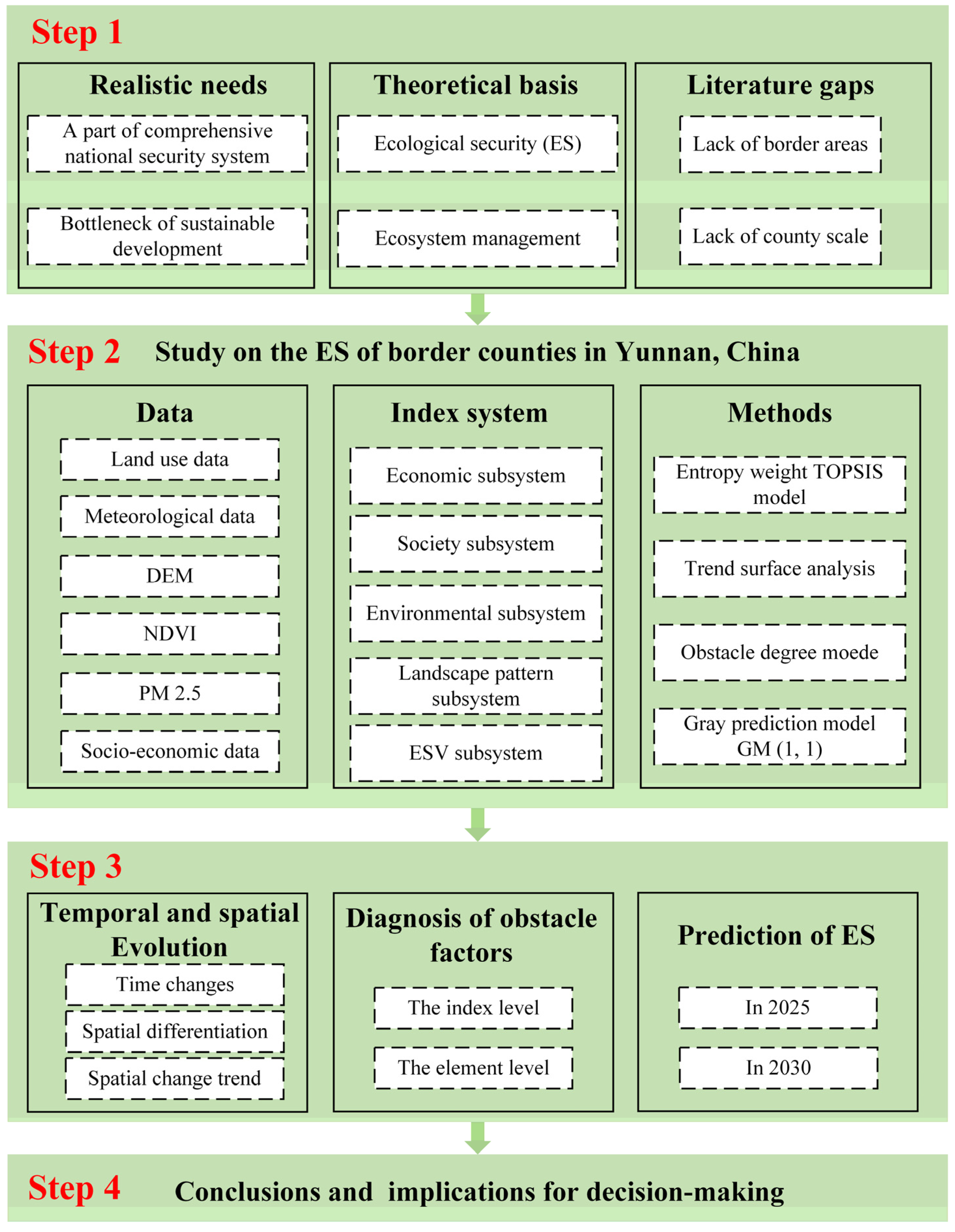
3.1. Research Framework

This study was conducted within a framework of four steps (Figure 2): the first step introduces the realistic needs, theoretical basis, and literature gaps related to ES. Then, the paper describes the study area and data sources, constructs an evaluation index system for ES, and introduces the methods. The third step analyzes the results. The last step expounds the conclusions and policy implications.

3.2. Construction of the Index System

Ecological security is a complex system involving nature, the economy, and human society [20,42]; the level of ES in any area is constantly changing [30,43]. In the past, the assessment of ES generally involved the construction of an index system from the perspective of ecosystem structure and function [12], but it did not consider human beings as external factors. In reality, human beings have already become an indispensable part of the Earth’s ES system. Supporting the sustainable development of the economy and society is an important reason to study ES [43]. Therefore, the present study evaluates the state of ES in border areas from five subsystems: economy, society, environment, landscape pattern, and ecosystem service value (ESV). The process of calculating the landscape patterns and ESVs is as follows:

(1) Selection and calculation of landscape metrics.

The evolution of landscape pattern leads to spatial changes in the landscape results, which directly reflect the changes in ecosystem structure and composition and finally affect ES [18]. A landscape index can describe the change in landscape pattern. Landscape indices are used to determine the relationship between landscape pattern and the process of landscape change [36]. In this study, the number of patches (NP), patch density (PD), largest patch index (LPI), edge density (ED), landscape shape index (LSI), splitting index (SPLIT), Shannon’s diversity index (SHDI), and aggregation index (AI) were selected to reflect the level of landscape pattern subsystem [44,45]. The selected landscape index was calculated using FRAGSTATS 4.2 software.

(2) Calculation of ESV.

Ecological security depends on the level of ecosystem services provided by an ecosystem to human beings [46]. At present, ES has become an important research topic designed to bring ecosystem services into the evaluation of ES systems [46,47]. In 1997, Costanza et al. [48] put forward the method of evaluating global scale ecosystem services with ESV, and Xie, a Chinese scholar [49], summarized an equivalent factor of ESV per unit area according to the actual situation of China. In this study, we referred to their methods and modified the above-mentioned equivalent factor. For the border areas analyzed here, the following standards were used: cropland corresponds to dry land; the equivalent factor for forest is taken as the average value of coniferous, mixed, and broad-leaved forests; grassland corresponds to prairie; snow/ice corresponds to glacier and snow [50]; and impervious areas were assigned “0” [51] (Table S1).

The economic value of one ecological service equivalence factor is 1/7 the grain output value per unit area [49], and the economic value of the equivalent factor in border areas was calculated according to Equation (1). To eliminate the impact of crop price fluctuation on the total value, the area, yield, and average price of the three main crops (rice, corn, and wheat) were selected as the basic data. The calculation process is as follows:

$$V{C}_0=\frac{1}{7}{\displaystyle \sum _{i=1}^n\frac{m_i{p}_i{q}_i}{M}}\left(n=1,2,3\right)$$

(1)

According to Equation (1), the economic value of one equivalent factor of ESV in border areas is 1817.76 yuan/ha, and the ESV coefficient per unit area of land use type was obtained (Table S2). Referring to the method of Hu et al. [36], the sensitivity index of the ESV coefficient for all land use types was obtained (Table S3). The sensitivity index of the ESV coefficient was all less than 1, which indicates that the estimated total ESV in the study area is not elastic to the equivalent factor.

The index system of ES is shown in

Table 2. The index system of ecological security evaluation in border areas.

Target Layer	Elements Layer	Index Layer	References
ES	Economic subsystem	X1: Annual GDP growth rate (%)	[52]
		X2: Per-capita GDP (yuan)	[22]
		X3: Secondary industry as percentage of GDP (%)	[53]
		X4: Tertiary industry as percentage of GDP (%)	[25]
		X5: Fixed assets investment (104 yuan)	[18]
		X6: Per-capita fiscal revenue (yuan)	[25]
	Society subsystem	X7: Population growth rate (%)	[24]
		X8: Population density (person/square kilometer)	[24,52]
		X9: Per-capita food production (tons/person)	[22]
		X10: Number of medical beds per 10,000 persons (pieces/ten thousand people)	[25]
		X11: Urbanization level (%)	[43]
	Environment subsystem	X12: Annual average temperature (°C)	[43]
		X13: Annual precipitation (mm)	[43]
		X14: PM2.5 (μg/m3)	[24]
		X15: NDVI (/)	[18]
		X16: Forest cover (%)	[25]
		X17: Proportion of construction land (%)	[26]
		X18: Proportion of cultivated land (%)	[25]
	Landscape pattern subsystem	X19: NP (/)	[54]
		X20: PD (/)	[12,43]
		X21: LPI (/)	[43]
		X22: ED (/)	[12]
		X23: LSI (/)	[54,55]
		X24: SPLIT (/)	[12,43]
		X25: SHDI (/)	[12,43]
		X26: AI (/)	[54,55]
	ESV subsystem	X27: Food production (104 yuan)	[24,50]
		X28: Raw material (104 yuan)	[24,50]
		X29: Water supply (104 yuan)	[24,50]
		X30: Air quality regulation (104 yuan)	[24,50]
		X31: Climate regulation (104 yuan)	[24,50]
		X32: Waste treatment (104 yuan)	[24,50]
		X33: Water regulation (104 yuan)	[24,50]
		X34: Erosion prevention (104 yuan)	[24,50]
		X35: Soil fertility maintenance (104 yuan)	[24,50]
		X36: Habitat services (104 yuan)	[24,50]
		X37: Cultural services (104 yuan)	[24,50]

.

3.3. Entropy Weight TOPSIS Model

The entropy weight method is an objective weighting method, which uses entropy to indicate the information’s size. Generally, the larger the gap between feature values, the larger the size of information it possesses [56]. The technique for order preference by similarity to ideal solution (TOPSIS) is a multi-objective decision-making method. The principle is to rank the evaluation objects according to the closeness of positive and negative ideal solutions. At present, the combination of entropy weight method and TOPSIS method has been widely used in land use planning, sustainable development assessment, and other fields [57,58]. This study selected entropy weight TOPSIS model to evaluate the level of the ES in border areas. The calculation process is as follows:

(1) Data standardization was completed using the following equation:

$$\{\begin{array}{l}{g}_{ij}=\frac{y_{ij}-y_{min}}{y_{max}-y_{min}}, where{g}_{ij}isapositiveindicator\\ g_{ij}=\frac{y_{max}-y_{ij}}{y_{max}-y_{min}},where{g}_{ij}isanegativeindicator\end{array}$$

(2)

where g_ij is the normalized value; and y_max and y_min represent the maximum and minimum values of the j^th index, respectively.

(2) The information entropy of each index was calculated using the following equation:

$$H_j=-\frac{1}{\ln n}\left({\displaystyle \sum _{i=1}^n{f}_{ij}\ln f_{ij}}\right)$$

(3)

where $f_{ij}=\left(1+g_{ij}\right)/\left[{\displaystyle \sum _{i=1}^n\left(1+g_{ij}\right)}\right]$.

(3) The index weights were determined using the following equation:

$$w_j=\frac{1-H_j}{m-{\displaystyle \sum _{j=1}^m{H}_j}}$$

(4)

(4) The weight normalization matrix was constructed using the following equation:

$$c_{ij}=g_{ij}\ast w_j$$

(5)

where c_ij is the weighted normalized decision matrix; and w_j is the weight value of the j^th index.

(5) The positive and negative ideal solutions, C⁺ and C⁻, respectively, were calculated using the following equation:

$$\{\begin{array}{l}{C}^{+}=\left\{\underset{1\le i\le m}{\max c_{ij}|i=1,2,\cdots ,m}\right\}=\left\{c_1{}^{+},c_2{}^{+},\cdots ,c_j{}^{+}\right\}\\ C^{-}=\left\{\underset{1\le i\le m}{\min c_{ij}|i=1,2,\cdots ,m}\right\}=\left\{c_1{}^{-},c_2{}^{-},\cdots ,c_j{}^{-}\right\}\end{array}$$

(6)

where C⁺ and C⁻ refer to the optimal and the least considered decision schemes, respectively.

(6) The distance from the index value of each evaluation object to C⁺ and C⁻ was calculated using the following equations:

$$\{\begin{array}{l}{S}_j{}^{+}=\sqrt{{\displaystyle \sum _{j=1}^n{\left(c_j{}^{+}-c_{ij}\right)}^2}},i=1,2,\cdots ,m\\ S_j{}^{-}=\sqrt{{\displaystyle \sum _{j=1}^n{\left(c_j{}^{-}-c_{ij}\right)}^2}},i=1,2,\cdots ,m\end{array}$$

(7)

where S_j⁺ and S_j⁻ refer to the distance of the assessment vector to the positive and negative ideal solutions, respectively.

(7) The closeness of each evaluation object to the ideal solution was calculated using the following equation:

$$R_i=\frac{S_j{}^{-}}{S_i{}^{+}+S_i{}^{-}}$$

(8)

where R_i is the closeness of the evaluation object to the optimal solution, and the range of R_i is 0–1. The greater the value of R_i, the higher the ES level. Referring to the research of Cui et al. [59], we divided the level of ES into five levels (

Table 3. Evaluation criteria of ecological security.

Range	Status	Characteristics
[0, 0.25)	Critical	The pressure on the ecosystem is very large, the ecosystem structure is very imperfect, and the ecosystem has a very large risk of collapse.
[0.25, 0.45)	Unstable	The pressure on the ecosystem is large; the ecosystem structure has defects and is in an unstable state.
[0.45, 0.55)	Sensitive	The pressure on the ecosystem is large and close to the threshold; the ecosystem structure is relatively complete and can play the basic function of the ecosystem.
[0.55, 0.75)	Good	The ecosystem has relatively little pressure and perfect functions, and the ecosystem is in a relatively stable state.
[0.75, 1]	Secure	The pressure on the ecosystem is very small, the ecological function and structure are in excellent condition, and the ecosystem is in a very stable state.

).

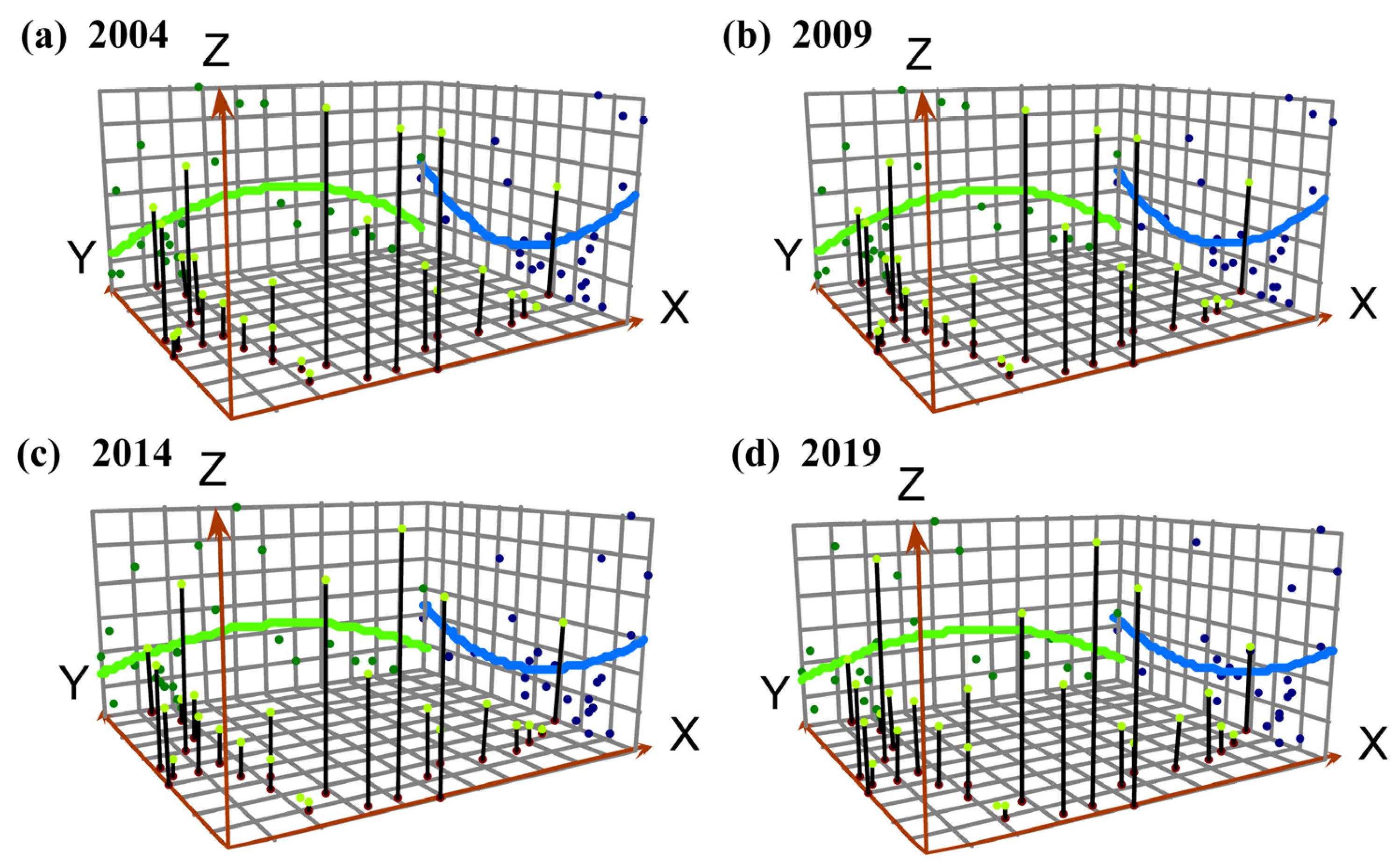
3.4. Trend Surface Analysis

Trend surface analysis is a method that can be used to simulate the spatial distribution law and change trend in geographical elements with a smooth mathematical surface [60]. The actual surface is divided into two components: a regional trend and residual values. The regional trend is calculated by using a polynomial surface with continuous power, and the residual values are the arithmetic difference between the original data and the trend surface, indicating local fluctuations. This study used this method to analyze the spatial differentiation trend in ES [61], as follows:

$$Z_i\left(x_i,y_i\right)=T_i\left(x_i,y_i\right)+{\epsilon }_i$$

(9)

where Z_i(x_i, y_i), T_i(x_i, y_i), and ε_i represent the observed, trend, and residual values of variable Z at location (x_i, y_i), respectively.

3.5. Obstacle Degree Model

Based on the ES evaluation of border areas, identifying the key factors that directly influence the ES can help to present adaptation measures designed to help land managers preferably maintain the ES in border areas and promote sustainable regional development. Therefore, our study used an obstacle degree model to analyze the factors creating obstacles and influencing ES. The calculation process is as follows [62]:

$$P_{ij}=1-g_{ij}$$

(10)

$$M_{ij}=\frac{R_{ij}{P}_{ij}}{{\displaystyle \sum _{i,j=1}^m{R}_{ij}{P}_{ij}}}\times 100\%$$

(11)

where M_ij represents the obstacle degree of the i^th indicator in year j, and P_ij is the degree of deviation for indicator i in year j.

3.6. GM (1,1) Gray Prediction Model

The gray system theory was first put forward by Deng [63]. A gray prediction model (GM) (1,1) adopts the basic concept of the gray system theory and has been widely used in the fields of ecology and social economics [64,65]. It has unique advantages in predicting and analyzing objects and process systems with small amounts of data, no obvious change law of data, has an unclear structural relationship, and has an operation mechanism. The prediction calculation process is simple and accurate. Considering that the change in ES has fuzzy and uncertain characteristics [43], and predicting its change is a typical gray evaluation process, GM (1,1) is selected to predict the ES level of border areas in 2025 and 2030. The calculation process is as follows:

(1) Preprocess the data. The original sequence $Y_i{}^{\left(0\right)}$ of all data from 2004 to 2019 is set as follows:

$$Y_i{}^{\left(0\right)}=\left[Y_i{}^{\left(0\right)}\left(1\right),Y_i{}^{\left(0\right)}\left(2\right),\cdots ,Y_i{}^{\left(0\right)}\left(16\right)\right]$$

(12)

Use Equation (13) to obtain a new sequence $Y_{\mathrm{i}}{}^{\left(1\right)}\left(k\right)$:

$$Y_i{}^{\left(1\right)}\left(k\right)={\displaystyle \sum _{i=1}^k{Y}_i{}^{\left(0\right)}=Y_i{}^{\left(1\right)}\left(k-1\right)}+Y_i{}^{\left(0\right)}\left(k\right)$$

(13)

$$Y_i{}^{\left(1\right)}=\left[Y_i{}^{\left(1\right)}\left(1\right),Y_i{}^{\left(1\right)}\left(2\right),\cdots ,Y_i{}^{\left(1\right)}\left(16\right)\right]$$

(14)

(2) Set up the gray differential equation:

$$Y_i{}^{\left(1\right)}\left(k+1\right)=\left[Y_i{}^{\left(0\right)}-\frac{b}{a}\right]e^{-ak}+\frac{b}{a}$$

(15)

where the values of parameters a and b are calculated by the least squares method [66].

(3) Predict the data. Based on Equation (16), the ES level of border areas in 2025 and 2030 is predicted as follows:

$${\stackrel{\wedge }{Y}}_i{}^{\left(0\right)}\left(k+1\right)={\stackrel{\wedge }{Y}}_i{}^{\left(1\right)}\left(k+1\right)-{\stackrel{\wedge }{Y_i}}^{\left(1\right)}\left(k\right)$$

(16)

(4) Test the accuracy of the prediction data. After the fitting value ${\stackrel{\wedge }{Y}}_i{}^{\left(0\right)}$ of ES is obtained using Equation (16), the correctness of the model needs to be tested according to the original $Y_i{}^{\left(0\right)}$ and fitting ${\stackrel{\wedge }{Y}}_i{}^{\left(0\right)}$ sequences. The mean absolute percent error (MAPE) is usually used to test the accuracy of the model:

$$MAPE=\frac{1}{n}{\displaystyle \sum _{k=1}^n\left|\frac{Y_i{}^{\left(0\right)}\left(k\right)-{\stackrel{\wedge }{Y_i}}^{\left(0\right)}\left(k\right)}{Y_i{}^{\left(0\right)}\left(k\right)}\right|}$$

(17)

We referred to the studies of Wang et al. [66] and Wang and Li [67]; when the MAPE is less than 10%, the forecasting is highly accurate. After calculation, the MAPE of all the data that were predicted in this paper was less than 10% (

Table 4. Mean absolute percent error (MAPE) for each county, which was used to test the accuracy of the model; a MAPE > 10% indicates that the predicted results are highly accurate.

County	Mape	County	Mape	County	Mape
Cangyuan	3.47%	Lancang	0.52%	Mengla	2.26%
Fugong	1.51%	Longling	4.47%	Menglian	1.91%
Funing	0.80%	Longchuan	1.41%	Ruili	4.25%
Gengma	3.28%	Lushui	2.03%	Tengchong	2.23%
Gongshan	1.43%	Lvchun	2.81%	Ximeng	1.59%
Hekou	5.93%	Malipo	1.69%	Yingjiang	0.80%
Jiangcheng	0.74%	Maguan	3.14%	Zhenkang	2.98%
Jinping	1.87%	Mangshi	1.45%
Jinghong	2.71%	Menghai	1.46%

), which meets the requirement needed to verify prediction accuracy.

4. Results

4.1. Temporal Changes in ES

Based on an entropy weight TOPSIS model, we calculated the ES of each border county. From 2004 to 2019, the ES of all border counties showed a positive upward trend (Figure 3). Tengchong, Jinghong, and Ruili ranked among the top three counties in terms of the increase in ES. Among them, the ES of Tengchong increased from 0.4124 in 2004 to 0.6417 in 2019, an increase of 0.2294. The ES of Jinghong increased from 0.4798 in 2004 to 0.6882 in 2019, an increase of 0.2084. The ES of Ruili increased from 0.1994 in 2004 to 0.3537 in 2019, an increase of 0.1544.

We also analyzed the time trend in five subsystems, namely, the economic, social, environmental, landscape pattern, and the ecosystem service value subsystems (Figure 3). All border counties generally showed an upward trend for their economic and social subsystems, with the economic subsystem of Tengchong rising the most, from 0.1186 in 2004 to 0.6871 in 2019, an increase of 0.5685. The social subsystem of Mangshi rose the most, from 0.3296 in 2004 to 0.7634 in 2019, an increase of 0.4338. The counties of Cangyuan, Fugong, Funing, Gengma, Jinping, Jinghong, Longchuan, Lvchun, Malipo, Menghai, Mengla, Menglian, and Yingjiang showed a fluctuating upward trend in their environmental subsystems, while the level of the environmental subsystems of other counties generally decreased. Jinping experienced the largest increase in terms of landscape pattern subsystem, from 0.3966 in 2004 to 0.5095 in 2019, an increase of 0.1128. the ESV subsystem of all border counties changed little during the study period.

4.2. Spatial Changes in ES

Our results show the spatial changes in ES in border areas in 2004, 2009, 2014, and 2019 (Figure 4). In 2004, the ES level of all border counties was lower than the good level, among which Lincang, Jinghong, and Mengla had the highest ES level and were classified as being in a sensitive state. In 2009, the level of ES in Mangshi changed from critical to the unstable state. In 2014, the level of ES in Jinghong first reached the good state. Tengchong changed from the unstable to the sensitive state, while Longling, Zhenkang, and Lvchun changed from the critical to the unstable state. In 2019, the number of border counties in the critical state had decreased, with only Ximeng, Menglian, and Malipo in the critical state, showing that the ES level in the southwestern part of the study area was higher than that in the west and east.

Based on the evaluation of ES in 2004, 2009, 2014, and 2019, the Geostatistical Analyst tool in ArcGIS 10.7 was applied to visualize the spatial representation of ES conditions. A spatial change trend map of the ES was obtained thereby (Figure 5). The X and Y axes indicate the east and north directions, respectively, while the Z-axis indicates the size of the ecological safety assessment value. The green and blue lines in Figure 5 represent the fitting curve of ES in the east–west and north–south directions [68]. In the east–west direction, the trend lines of the four years analyzed here remained stable, and all showed an “inverted U-shaped” distribution (Figure 5), characterized by the central part being higher than the western and eastern parts, while the western part was higher than the eastern part. In the north–south direction, the trend line changed from a “U-shaped” distribution to a “straight line,” characterized by higher values in the southern and northern parts than in the central part, while the gap has become significantly narrow; the ES of the northern part has always remained lower than that of the southern part. These results are consistent with the spatial distribution pattern of high in the southwest and low in the east and west.

4.3. Diagnosis of Obstacle Factors for ES

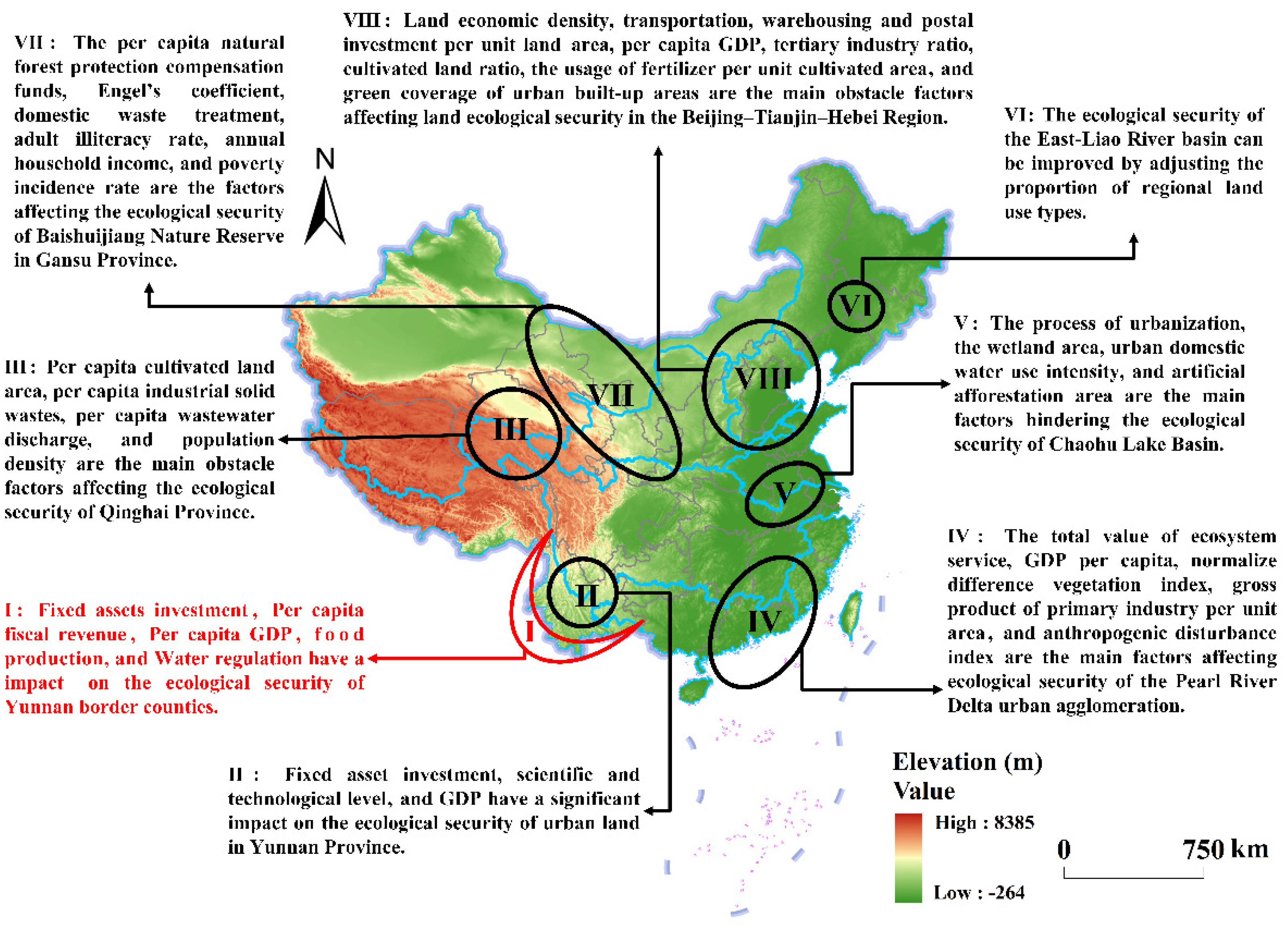
4.3.1. Analysis of Obstacle Factors at the Index Level

Based on the degree of obstacle model, the factors creating obstacles that affect ES in the studied border areas were determined (Figure 6; however, only the factors in 2004 and 2019 are listed). By analyzing the degree of obstacles for each factor [69], the five top obstacle factors were found to be the following: fixed asset investment (X5), per capita fiscal revenue (X6), per capita GDP (X2), food production (X27), and water regulation (X33). In 2004, the average obstacle degree of X5, X6, X2, X27, and X33 was 14.11%, 8.86%, 7.90%, 4.74%, and 4.21%, respectively. In 2019, the average obstacle degree of X5, X6, X2, X27, and X33 was 11.10%, 7.07%, 6.31%, 5.42%, and 4.73%, respectively.

4.3.2. Analysis of Obstacle Factors at the Element Level

Based on the calculations of the obstacle degree of each indicator, the obstacle degree of factors at the element level was also obtained (Figure 7). The obstacle degrees at the element level in border areas varied between 2004 and 2019. In 2004, the economic subsystem was the main obstacle to improving the ES in Jinghong, Lancang, and Mengla, while the ESV subsystem was the main obstacle to improving the ES in the other 22 border counties. In 2019, the obstacle degree of the economic subsystem increased in Langcang, while the obstacle degree of the economic subsystem of all the other 24 border counties decreased. The obstacle degrees of social, environmental, and landscape pattern subsystems changed little.

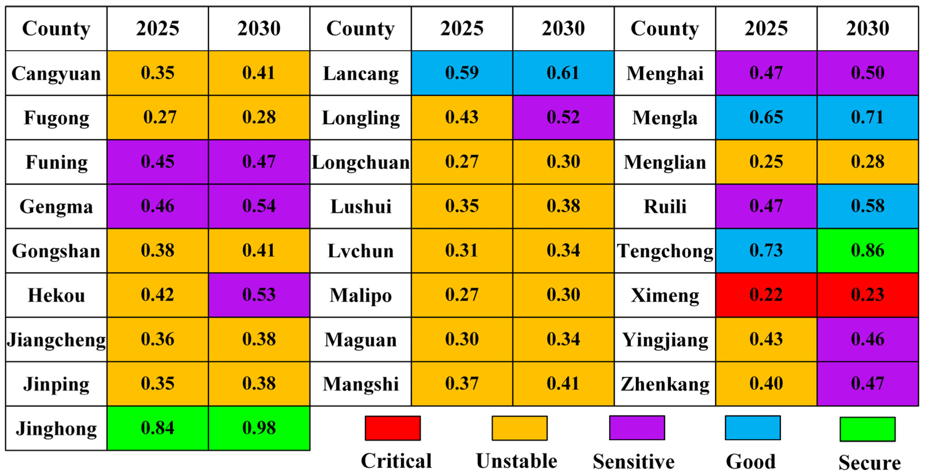
4.4. Prediction of Changes in ES for the Period 2025–2030

According to the respective ES level of each border county from 2004 to 2019, predicted values for ES in 2025 and 2030 were obtained (Figure 8). The ES of border areas is predicted to maintain an upward trend. In 2025, Jinghong would first reach a secure state; Lancang, Mengla, and Tengchong would reach a good state; and Menghai, Ruili, Gengma and Funing would reach a sensitive state. Ximeng would maintain a critical state, and the other 16 counties would be in an unstable state. In 2030, Jinghong and Tengchong would reach a secure state; Lancang, Mengla, and Ruili would reach a good state; and Funing, Gengma, Hekou, Longling, Menghai, Yingjiang, and Zhenkang would reach a sensitive state. Cangyuan, Fugong, and another 10 counties would be in an unstable state. However, Ximeng would remain in a critical state.

5. Discussion

5.1. Discussion of Change in ES

The main objective of this study was to analyze the ES of 25 counties with international borders in Yunnan Province, China. First, we selected these 25 counties as the case study area and constructed an index system to evaluate the ES from the five subsystems of economy, society, environment, landscape pattern, and ESV. We found that human and natural systems interact to affect the ES, which is consistent with previous studies [30]. Efforts related to ecological protection need to be coordinated with social and economic development, which can provide more comprehensive guidance for land management by environmental decision makers [70,71]. Second, we found that the ES of border areas showed a spatial distribution pattern of high in the southwest and low in the west and east. Jinghong had the highest level of ES, because Jinghong has adhered to the implementation of a project designed to return rubber plantation land to forest and has delimited an ecological red line, resulting in the ES of Jinghong ranking first among the border counties. Third, we found that from 2004 to 2019, the ES of border areas showed an overall upward trend, indicating that remarkable achievements have been made in ecological protection in Yunnan Province. However, on the premise of maintaining the existing development mode, we predicted the ES status of border areas in 2025 and 2030. We found that only one county will reach the classification of secure status in 2025 and two counties will reach the secure status in 2030, which is still a certain distance from the goal of establishing an ES barrier. Therefore, local governments should continue to pay more attention to the ES in border areas and formulate environmental policies according to the natural endowment and economic development of border areas.

5.2. Discussion on Obstacle Factors

In China, significant differences in socio-economic development and natural conditions among regions have caused the factors influencing ES in different regions to vary [12,17,22,26,72,73,74,75] (Figure 9). For the border areas in Yunnan Province, we found that the fixed asset investment, per capita fiscal revenue, per capital GDP, and food production are the main factors creating obstacles to improving the level of ES, which is consistent with previous research results [73]. Fixed asset investment plays a major role in promoting both the economy and the upgrading of industrial infrastructure, so as to reduce the pressure of industrial development on the environment. The higher the per-capita GDP and fiscal revenue, the more capable people are of protecting the environment. In addition, the border areas are located in the upstream regions of the Nujiang, Lancang, and other rivers. This region serves as an important area for supplying and regulating water resources in Asia [10]. Therefore, the capacity to regulate water availability significantly affects the ES in border areas. In short, economic development and the provision of water-related ecosystem services are the main factors creating obstacles that affect the ES in border areas.

5.3. Limitations and Implications

This study has several limitations and can be improved in future research. First, biodiversity is an important embodiment of ES, especially in border areas of Yunnan Province, a global biodiversity hotspot. However, biodiversity data are difficult to obtain at the county scale. In the future work, the indicators for measuring biodiversity need to be further considered. Second, when predicting the ES of border areas, this study only considered the state that the border areas are predicted to reach in 2025 and 2030 under the situation of maintaining the existing development mode, but did not consider multiple scenarios, such as models of existing development and priorities in economic and environmental development, to simulate the future ES of border areas. Future research should make up for these shortcomings.

In the process of national development, as the border areas were far away from the political and economic center of the country in the past, previous studies often ignored the border areas [76]. With the acceleration in globalization, the border areas have changed from the original inferior states to the area with increasingly close international cooperation. The border areas of Yunnan Province, China, border on Myanmar, Laos, and Vietnam, and belong to the upstream area of many international rivers [35]. The situation in this area is relatively complicated. Selecting this area as the research case can provide reference for researchers to study the ES of border areas. This study finds that the Chinese government has effectively improved the level of ES in the border areas by implementing a series of environmental protection policies [77]. Therefore, other countries can also achieve the purpose of protecting the ecosystem by continuously increasing their attention to the ES in the border areas. However, the national boundaries divided by administrative units are not necessarily the boundaries of natural ecosystems. Carrying out mutual cooperation among countries is also an important way to improve the ES of border areas. In terms of specific implementation, first, it is essential to pay attention to the ecological restoration and protection measures in the most valuable areas [78]. By distinguishing the differences in the level of ES in different regions of the study area, it helps the local government to choose the priority of policy implementation. Second, when implementing environmental protection policies, the local government should identify the obstacle factors affecting the ES in advance, so as to implement environmental policies pertinently. Third, as an important basis for a comprehensive national security system, the amount of research on the ES of border areas needs to be increased, so as to provide reference for local environmental decision making.

6. Conclusions

Improving the ES of border areas is of great significance to local sustainable development [10]. However, few studies have addressed the status of ES in border areas, especially on the county scale [79]. Therefore, 25 border counties in Yunnan Province were selected as the study case. We used an entropy weight TOPSIS model to evaluate the ES conditions of border areas from 2004 to 2019 and used trend surface analysis to evaluate the spatial differentiation trends. Then, we diagnosed the factors creating obstacles that affect ES and used a GM (1,1) model to predict the state of ES in both 2025 and 2030. The results show the following patterns:

(1) From 2004 to 2019, the level of ES in all border counties showed a positive upward trend. Tengchong, Jinghong, and Ruili counties ranked among the top three in terms of the improved ES, with increases of 0.2294, 0.2084, and 0.1544, respectively. In terms of five subsystems (economy, society, environment, landscape pattern, and ecosystem service value), the 25 counties had obvious differences. The levels of the economic and social subsystems showed an overall upward trend; the levels of environmental and landscape pattern subsystems fluctuated continuously; and the overall change in the ESV subsystem was small.

(2) The ES of border areas presented a spatial distribution pattern of high in the southwest and low in the west and east. The level of ES in Lancang was the highest in 2004 and 2009 and that of Jinghong was the highest in 2014 and 2019. The trend of spatial change in ES in border areas generally presented the characteristics of remaining stable in the east–west direction and changing in the north–south direction.

(3) In terms of index level, fixed asset investment, fiscal revenue, per-capita GDP, food production, and water regulation are the top five obstacles to improving the ES in border areas. In terms of element level, the economic subsystem is the main factor creating an obstacle to improving the ES in Jinghong, Lancang, and Mengla, while the ESV subsystem is the main factor affecting improvement in the ES in the other 22 counties.

(4) The gray prediction model GM (1,1) can effectively predict the future situation of border areas in both 2025 and 2030. The level of ES in border areas is predicted to maintain an upward trend. In 2025, the ES in Jinghong will reach 0.84 and will be in a secure state. By 2030, the number of border counties with a secure state of ES will increase to two, namely Jinghong and Tengchong. Their ES level will reach 0.98 and 0.86, respectively.

Our research provides reliable information on the ES of 25 border counties in Yunnan and puts forward targeted policy suggestions based on the research results, which will be necessary if China desires to implement sustainable development planning and management at the smallest administrative scale. In addition, this study can provide a reference for other countries to improve the level of ES in border areas.

References

1. Lambin, E.F.; Meyfroidt, P. Global land use change, economic globalization, and the looming land scarcity. Proc. Natl. Acad. Sci. USA 2011, 108, 3465. [Google Scholar] [CrossRef] [PubMed]
2. Weidenfeld, A. Tourism and cross border regional innovation systems. Ann. Tour. Res. 2013, 42, 191–213. [Google Scholar] [CrossRef]
3. Edzes, A.J.E.; van Dijk, J.; Broersma, L. Does cross-border commuting between EU-countries reduce inequality? Appl. Geogr. 2022, 139, 102639. [Google Scholar] [CrossRef]
4. Duan, W.L.; Zou, S.; Chen, Y.N.; Nover, D.; Fang, G.H.; Wang, Y. Sustainable water management for cross-border resources: The Balkhash Lake Basin of Central Asia, 1931–2015. J. Clean. Prod. 2020, 263, 121614. [Google Scholar] [CrossRef]
5. Su, X.B.; Li, C.S. Bordering dynamics and the geopolitics of cross-border tourism between China and Myanmar. Political Geogr. 2021, 86, 102372. [Google Scholar] [CrossRef]
6. Johnson, C.; Jones, R.; Paasi, A.; Amoore, L.; Mountz, A.; Salter, M.; Rumford, C. Interventions on rethinking ‘the border’ in border studies. Political Geogr. 2011, 30, 61–69. [Google Scholar] [CrossRef]
7. Newman, D. The lines that continue to separate us: Borders in our ‘borderless’ world. Prog. Hum. Geog. 2006, 30, 143–161. [Google Scholar] [CrossRef]
8. Laako, H.; Kauffer, E. Between colonising waters and extracting forest fronts: Entangled eco-frontiers in the Usumacinta River Basin. Political Geogr. 2022, 96, 102566. [Google Scholar] [CrossRef]
9. Chen, D.N.; Cai, Y.P.; Wang, X.; Li, C.H.; Yin, X.N.; Liu, Q. An inexact modeling approach for supporting water resources allocation under natural and social complexities in a border city of China and Myanmar. Resour. Conserv. Recycl. 2021, 168, 105245. [Google Scholar] [CrossRef]
10. He, D.M.; Wu, R.D.; Feng, Y.; Li, Y.G.; Ding, C.Z.; Wang, W.L.; Yu, D.W. REVIEW: China’s transboundary waters: New paradigms for water and ecological security through applied ecology. J. Appl. Ecol. 2014, 51, 1159–1168. [Google Scholar] [CrossRef]
11. Liu, J.; Wu, R.D.; He, D.M. Transboundary eco-security regulation for geopolitical cooperation in land border areas. Geogr. Program 2015, 34, 606–616. [Google Scholar]
12. Li, Z.T.; Yuan, M.J.; Hu, M.M.; Wang, Y.F.; Xia, B.C. Evaluation of ecological security and influencing factors analysis based on robustness analysis and the BP-DEMALTE model: A case study of the Pearl River Delta urban agglomeration. Ecol. Indicat. 2019, 101, 595–602. [Google Scholar] [CrossRef]
13. Norton, S.B.; Rodier, D.J.; van der Schalie, W.H.; Wood, W.P.; Slimak, M.W.; Gentile, J.H. A framework for ecological risk assessment at the EPA. Environ. Toxicol. Chem. 1992, 11, 1663–1672. [Google Scholar] [CrossRef]
14. Dai, Y.C.; Peng, G.C.; Wen, C.H.; Zahoor, B.; Ma, X.D.; Hacker, C.E.; Xue, Y.D. Climate and land use changes shift the distribution and dispersal of two umbrella species in the Hindu Kush Himalayan region. Sci. Total Environ. 2021, 777, 146207. [Google Scholar] [CrossRef]
15. Kong, Y.; He, W.J.; Yuan, L.; Zhang, Z.F.; Gao, X.; Zhao, Y.E.; Mulugeta Degefu, D. Decoupling economic growth from water consumption in the Yangtze River Economic Belt, China. Ecol. Indicat. 2021, 123, 107344. [Google Scholar] [CrossRef]
16. Dai, L.; Liu, Y.B.; Luo, X.Y. Integrating the MCR and DOI models to construct an ecological security network for the urban agglomeration around Poyang Lake, China. Sci. Total Environ. 2021, 754, 141868. [Google Scholar] [CrossRef]
17. Tang, Y.S.; Zhao, X.Y.; Jiao, J.L. Ecological security assessment of Chaohu Lake Basin of China in the context of River Chief System reform. Environ. Sci. Pollut. Res. 2020, 27, 2773–2785. [Google Scholar] [CrossRef]
18. Ma, L.B.; Bo, J.; Li, X.Y.; Fang, F.; Cheng, W.J. Identifying key landscape pattern indices influencing the ecological security of inland river basin: The middle and lower reaches of Shule River Basin as an example. Sci. Total Environ. 2019, 674, 424–438. [Google Scholar] [CrossRef]
19. Onkal-Engin, G.; Demir, I.; Hiz, H. Assessment of urban air quality in Istanbul using fuzzy synthetic evaluation. Atmos. Environ. 2004, 38, 3809–3815. [Google Scholar] [CrossRef]
20. Wu, Y.Z.; Zhang, T.C.; Zhang, H.; Pan, T.; Ni, X.L.; Grydehøj, A.; Zhang, J.M. Factors influencing the ecological security of island cities: A neighborhood-scale study of Zhoushan Island, China. Sustain. Cities Soc. 2020, 55, 102029. [Google Scholar] [CrossRef]
21. Liu, T.; Wang, H.Z.; Wang, H.Z.; Xu, H. The spatiotemporal evolution of ecological security in China based on the ecological footprint model with localization of parameters. Ecol. Indicat. 2021, 126, 107636. [Google Scholar] [CrossRef]
22. Fan, Y.P.; Fang, C.L. Evolution process and obstacle factors of ecological security in western China, a case study of Qinghai province. Ecol. Indicat. 2020, 117, 106659. [Google Scholar] [CrossRef]
23. Sun, M.Y.; Li, X.H.; Yang, R.J.; Zhang, Y.; Zhang, L.; Song, Z.W.; Liu, Q.; Zhao, D. Comprehensive partitions and different strategies based on ecological security and economic development in Guizhou Province, China. J. Clean. Prod. 2020, 274, 122794. [Google Scholar] [CrossRef]
24. Peng, C.C.; Li, B.; Nan, B. An analysis framework for the ecological security of urban agglomeration: A case study of the Beijing-Tianjin-Hebei urban agglomeration. J. Clean. Prod. 2021, 315, 128111. [Google Scholar] [CrossRef]
25. Cao, Y.H.; Liu, M.Y.; Zhang, Y.; Chen, C.; Cao, W.D. Spatiotemporal Evolution of Ecological Security in the Wanjiang City Belt, China. Chin. Geogr. Sci. 2020, 30, 1052–1064. [Google Scholar] [CrossRef]
26. Zhang, M.X.; Bao, Y.B.; Xu, J.; Han, A.; Liu, X.P.; Zhang, J.Q.; Tong, Z.J. Ecological security evaluation and ecological regulation approach of East-Liao River basin based on ecological function area. Ecol. Indicat. 2021, 132, 108255. [Google Scholar] [CrossRef]
27. Ghosh, S.; Das Chatterjee, N.; Dinda, S. Urban ecological security assessment and forecasting using integrated DEMATEL-ANP and CA-Markov models: A case study on Kolkata Metropolitan Area, India. Sustain. Cities Soc. 2021, 68, 102773. [Google Scholar] [CrossRef]
28. Ziegler Alan, D.; Fox Jefferson, M.; Xu, J. The Rubber Juggernaut. Science 2009, 324, 1024–1025. [Google Scholar] [CrossRef]
29. Foley, S. Threats to Mekong Forest Ecosystems: Last Chance for the Indo-Burma Biodiversity Hotspot, in Encyclopedia of the World’s Biomes; Goldstein, M.I., DellaSala, D.A., Eds.; Elsevier: Oxford, UK, 2020; pp. 168–184. [Google Scholar]
30. Wu, X.; Liu, S.L.; Sun, Y.X.; An, Y.; Dong, S.K.; Liu, G.H. Ecological security evaluation based on entropy matter-element model: A case study of Kunming city, southwest China. Ecol. Indicat. 2019, 102, 469–478. [Google Scholar] [CrossRef]
31. Bai, Y.; Wong, C.P.; Jiang, B.; Hughes, A.C.; Wang, M.; Wang, Q. Developing China’s Ecological Redline Policy using ecosystem services assessments for land use planning. Nat. Commun. 2018, 9, 3034. [Google Scholar] [CrossRef]
32. Gao, J.Y.; Castelletti, A.; Burlado, P.; Wang, H.; Zhao, J.S. Soft-cooperation via data sharing eases transboundary conflicts in the Lancang-Mekong River Basin. J. Hydrol. 2022, 606, 127464. [Google Scholar] [CrossRef]
33. Zanzanaini, C.; Trần, B.T.; Singh, C.; Hart, A.; Milder, J.; DeClerck, F. Integrated landscape initiatives for agriculture, livelihoods and ecosystem conservation: An assessment of experiences from South and Southeast Asia. Landsc. Urban Plan. 2017, 165, 11–21. [Google Scholar] [CrossRef]
34. Immerzeel Walter, W.; van Beek Ludovicus, P.H.; Bierkens Marc, F.P. Climate Change Will Affect the Asian Water Towers. Science 2010, 328, 1382–1385. [Google Scholar] [CrossRef]
35. Peng, J.; Yang, Y.; Liu, Y.X.; Hu, Y.N.; Du, Y.Y.; Meersmans, J.; Qiu, S.J. Linking ecosystem services and circuit theory to identify ecological security patterns. Sci. Total Environ. 2018, 644, 781–790. [Google Scholar] [CrossRef] [PubMed]
36. Hu, Z.N.; Yang, X.; Yang, J.J.; Yuan, J.; Zhang, Z.Y. Linking landscape pattern, ecosystem service value, and human well-being in Xishuangbanna, southwest China: Insights from a coupling coordination model. Glob. Ecol. Conserv. 2021, 27, e01583. [Google Scholar] [CrossRef]
37. Zhang, J.; Qu, M.; Wang, C.; Zhao, J.; Cao, Y. Quantifying landscape pattern and ecosystem service value changes: A case study at the county level in the Chinese Loess Plateau. Glob. Ecol. Conserv. 2020, 23, e01110. [Google Scholar] [CrossRef]
38. Myers, N.; Mittermeier, R.A.; Mittermeier, C.G.; da Fonseca, G.A.B.; Kent, J. Biodiversity hotspots for conservation priorities. Nature 2000, 403, 853–858. [Google Scholar] [CrossRef]
39. Gao, J.; Ryan, C.; Cave, J.; Zhang, C.Z. Tourism border-making: A political economy of China’s border tourism. Ann. Tour. Res. 2019, 76, 1–13. [Google Scholar] [CrossRef]
40. Yang, J.; Huang, X. The 30 m annual land cover dataset and its dynamics in China from 1990 to 2019. Earth Syst. Sci. Data 2021, 13, 3907–3925. [Google Scholar] [CrossRef]
41. Hammer, M.S.; van Donkelaar, A.; Li, C.; Lyapustin, A.; Sayer, A.M.; Hsu, N.C.; Levy, R.C.; Garay, M.J.; Kalashnikova, O.V.; Kahn, R.A.; et al. Global Estimates and Long-Term Trends of Fine Particulate Matter Concentrations (1998–2018). Environ. Sci. Technol. 2020, 54, 7879–7890. [Google Scholar] [CrossRef]
42. Yang, Y.J.; Song, G.; Lu, S. Assessment of land ecosystem health with Monte Carlo simulation: A case study in Qiqihaer, China. J. Clean. Prod. 2020, 250, 119522. [Google Scholar] [CrossRef]
43. Chen, Y.; Wang, J.L. Ecological security early-warning in central Yunnan Province, China, based on the gray model. Ecol. Indicat. 2020, 111, 106000. [Google Scholar] [CrossRef]
44. Yi, D.; Guo, X.; Han, Y.; Guo, J.; Ou, M.; Zhao, X. Coupling Ecological Security Pattern Establishment and Construction Land Expansion Simulation for Urban Growth Boundary Delineation: Framework and Application. Land 2022, 11, 359. [Google Scholar] [CrossRef]
45. Liang, F.; Bai, M.; Hu, Q.; Lin, S.-H. Ecological Security and Ecosystem Quality: A Case Study of Xia-Zhang-Quan Metropolitan Area in China. Land 2022, 11, 707. [Google Scholar] [CrossRef]
46. Wang, Y.; Pan, J.H. Building ecological security patterns based on ecosystem services value reconstruction in an arid inland basin: A case study in Ganzhou District, NW China. J. Clean. Prod. 2019, 241, 118337. [Google Scholar] [CrossRef]
47. Gao, J.B.; Du, F.J.; Zuo, L.Y.; Jiang, Y. Integrating ecosystem services and rocky desertification into identification of karst ecological security pattern. Landsc. Ecol. 2021, 36, 2113–2133. [Google Scholar] [CrossRef]
48. Costanza, R.; d’Arge, R.; de Groot, R.; Farber, S.; Grasso, M.; Hannon, B.; Limburg, K.; Naeem, S.; O’Neill, R.V.; Paruelo, J.; et al. The value of the world’s ecosystem services and natural capital. Nature 1997, 387, 253–260. [Google Scholar] [CrossRef]
49. Xie, G.D.; Lu, C.X.; Leng, Y.F.; Zheng, D.; Li, S.C. Ecological assets valuation of the Tibetan Plateau. J. Nat. Resour. 2003, 18, 189–196. [Google Scholar]
50. Xie, G.D.; Zhang, C.X.; Zhen, L.; Zhang, L.M. Dynamic changes in the value of China’s ecosystem services. Ecosyst. Serv. 2017, 26, 146–154. [Google Scholar] [CrossRef]
51. Jiang, W.; Lü, Y.H.; Liu, Y.X.; Gao, W.W. Ecosystem service value of the Qinghai-Tibet Plateau significantly increased during 25 years. Ecosyst. Serv. 2020, 44, 101146. [Google Scholar] [CrossRef]
52. Ke, X.L.; Wang, X.Y.; Guo, H.X.; Yang, C.; Zhou, Q.; Mougharbel, A. Urban ecological security evaluation and spatial correlation research—Based on data analysis of 16 cities in Hubei Province of China. J. Clean. Prod. 2021, 311, 127613. [Google Scholar] [CrossRef]
53. Cheng, H.R.; Zhu, L.K.; Meng, J.J. Fuzzy evaluation of the ecological security of land resources in mainland China based on the Pressure-State-Response framework. Sci. Total Environ. 2022, 804, 150053. [Google Scholar] [CrossRef] [PubMed]
54. Wang, S.D.; Zhang, X.Y.; Wu, T.X.; Yang, Y.Y. The evolution of landscape ecological security in Beijing under the influence of different policies in recent decades. Sci. Total Environ. 2019, 646, 49–57. [Google Scholar] [CrossRef]
55. Yushanjiang, A.; Zhang, F.; Yu, H.Y.; Kung, H.-t. Quantifying the spatial correlations between landscape pattern and ecosystem service value: A case study in Ebinur Lake Basin, Xinjiang, China. Ecol. Eng. 2018, 113, 94–104. [Google Scholar] [CrossRef]
56. Shannon, C.E. A mathematical theory of communication. Bell Syst. Tech. J. 1948, 27, 379–423. [Google Scholar] [CrossRef]
57. Wang, Y.J.; Chen, H.; Long, R.Y.; Sun, Q.Q.; Jiang, S.Y.; Liu, B. Has the Sustainable Development Planning Policy Promoted the Green Transformation in China’s Resource-based Cities? Resour. Conserv. Recycl. 2022, 180, 106181. [Google Scholar] [CrossRef]
58. Xiao, Y.; Chai, J.X.; Wang, R.; Huang, H. Assessment and key factors of urban liveability in underdeveloped regions: A case study of the Loess Plateau, China. Sustain. Cities Soc. 2022, 79, 103674. [Google Scholar] [CrossRef]
59. Cui, X.Y.; Fang, L.; Wang, X.R.; Kang, J.F. Urban eco-security assessment in the urban agglomerations based on DPSIR model: A case study of Yangtze River Delta, China. Acta Ecol. Sin. 2020, 41, 302–319. [Google Scholar]
60. Wang, H.C.; Zuo, R.G. A comparative study of trend surface analysis and spectrum–area multifractal model to identify geochemical anomalies. J. Geochem. Explor. 2015, 155, 84–90. [Google Scholar] [CrossRef]
61. Lu, X.H.; Zhang, Y.W.; Lin, C.R.; Wu, F. Analysis and comprehensive evaluation of sustainable land use in China: Based on sustainable development goals framework. J. Clean. Prod. 2021, 310, 127205. [Google Scholar] [CrossRef]
62. Sun, Y.; Zhao, T.Y.; Xia, L. Spatial-temporal differentiation of carbon efficiency and coupling coordination degree of Chinese county territory and obstacles analysis. Sustain. Cities Soc. 2022, 76, 103429. [Google Scholar] [CrossRef]
63. Deng, J.L. Control problems of grey Systems. Syst. Control Lett. 1982, 1, 288–294. [Google Scholar] [CrossRef]
64. Lin, C.S.; Liou, F.M.; Huang, C.P. Grey forecasting model for CO2 emissions: A Taiwan study. Appl. Energ. 2011, 88, 3816–3820. [Google Scholar] [CrossRef]
65. Yang, G.C.; Shang, P.P.; He, L.C.; Zhang, Y.C.; Wang, Y.; Zhang, F.; Zhu, L.; Wang, Y. Interregional carbon compensation cost forecast and priority index calculation based on the theoretical carbon deficit: China as a case. Sci. Total Environ. 2019, 654, 786–800. [Google Scholar] [CrossRef] [PubMed]
66. Wang, X.L.; Wei, Y.W.; Shao, Q.L. Decomposing the decoupling of CO2 emissions and economic growth in China’s iron and steel industry. Resour. Conserv. Recycl. 2020, 152, 104509. [Google Scholar] [CrossRef]
67. Wang, Z.X.; Li, Q. Modelling the nonlinear relationship between CO2 emissions and economic growth using a PSO algorithm-based grey Verhulst model. J. Clean. Prod. 2019, 207, 214–224. [Google Scholar] [CrossRef]
68. Zheng, H.; Khan, Y.A.; Abbas, S.Z. Exploration on the coordinated development of urbanization and the eco-environmental system in central China. Environ. Res. 2022, 204, 112097. [Google Scholar] [CrossRef] [PubMed]
69. Chen, Y.; Zhu, M.K.; Lu, J.L.; Zhou, Q.; Ma, W.B. Evaluation of ecological city and analysis of obstacle factors under the background of high-quality development: Taking cities in the Yellow River Basin as examples. Ecol. Indicat. 2020, 118, 106771. [Google Scholar] [CrossRef]
70. Mooney, H.A.; Duraiappah, A.; Larigauderie, A. Evolution of natural and social science interactions in global change research programs. Proc. Natl. Acad. Sci. USA 2013, 110, 3665–3672. [Google Scholar] [CrossRef]
71. Wu, X.T.; Wei, Y.P.; Fu, B.J.; Wang, S.; Zhao, Y.; Moran Emilio, F. Evolution and effects of the social-ecological system over a millennium in China’s Loess Plateau. Sci. Adv. 2020, 6, eabc0276. [Google Scholar] [CrossRef]
72. Guo, D.Y.; Wang, D.Y.; Zhong, X.Y.; Yang, Y.Y.; Jiang, L.X. Spatiotemporal Changes of Land Ecological Security and Its Obstacle Indicators Diagnosis in the Beijing–Tianjin–Hebei Region. Land 2021, 10, 706. [Google Scholar] [CrossRef]
73. Yang, R.Y.; Du, W.Y.; Yang, Z.S. Spatiotemporal Evolution and Influencing Factors of Urban Land Ecological Security in Yunnan Province. Sustainability 2021, 13, 2936. [Google Scholar] [CrossRef]
74. Liu, Y.Y.; Zhao, C.Y.; Liu, X.M.; Chang, Y.P.; Wang, H.; Yang, J.H.; Yang, X.G.; Wei, Y. The multi-dimensional perspective of ecological security evaluation and drive mechanism for Baishuijiang National Nature Reserve, China. Ecol. Indicat. 2021, 132, 108295. [Google Scholar] [CrossRef]
75. Rao, Y.; Dai, J.; Dai, D.; He, Q.; Wang, H. Effect of Compactness of Urban Growth on Regional Landscape Ecological Security. Land 2021, 10, 848. [Google Scholar] [CrossRef]
76. Ackleson, J. Constructing security on the U.S.–Mexico border. Political Geogr. 2005, 24, 165–184. [Google Scholar] [CrossRef]
77. Sills, J.; Yin, D.; Yuan, Z.J.; Li, J.; Zhu, H. Mitigate human-wildlife conflict in China. Science 2021, 373, 500–501. [Google Scholar] [CrossRef]
78. Huang, L.Y.; Wang, J.; Fang, Y.; Zhai, T.L.; Cheng, H. An integrated approach towards spatial identification of restored and conserved priority areas of ecological network for implementation planning in metropolitan region. Sustain. Cities Soc. 2021, 69, 102865. [Google Scholar] [CrossRef]
79. Liu, C.; Li, W.; Xu, J.; Zhou, H.; Li, C.; Wang, W. Global trends and characteristics of ecological security research in the early 21st century: A literature review and bibliometric analysis. Ecol. Indicat. 2022, 137, 108734. [Google Scholar] [CrossRef]
Figure 1. Map of the study area location along the southern and western borders of Yunnan Province. An inset map shows the study area location within the provinces and other administrative areas of China. Note: Map was created by authors using ArcGIS 10.7 based on the digital elevation model (DEM) data from the Resources and Environment Data Center of the Chinese Academy of Sciences (https://www.resdc.cn/, accessed on 4 January 2022).
Land 11 00892 g001
Figure 2. The research framework used in this study.
Land 11 00892 g002
Figure 3. Evaluation scores for temporal changes in ecological security and subsystems (economic, social, environmental, landscape pattern, and ecosystem service value (ESV)) in 25 border counties of Yunnan Province, China.
Land 11 00892 g003
Figure 4. Spatial change in ecological security in 25 border counties in Yunnan Province, China for: (a) 2004; (b) 2009; (c) 2014; and (d) 2019. Note: Maps were created by authors using ArcGIS 10.7.
Land 11 00892 g004
Figure 5. Spatial change trend in ecological security in 25 border counties in Yunnan Province, China for: (a) 2004; (b) 2009; (c) 2014; and (d) 2019.
Land 11 00892 g005
Figure 6. The obstacle degree of each indicator of ecological security in 25 border counties in Yunnan Province, China in: (a) 2004 and (b) 2019 (%).
Land 11 00892 g006
Figure 7. The obstacle degree of each element of ecological security in 25 border counties in Yunnan Province, China for economic, social, environmental, landscape pattern, ecosystem service value (ESV). Note: 04 and 19 indicate the years of 2004 and 2019, respectively.
Land 11 00892 g007
Figure 8. Prediction of the ecological security in 25 border counties of Yunnan Province, China in 2025 and 2030.
Land 11 00892 g008
Figure 9. Spatial distribution of influencing factors of ecological security in China. Eight regions are labeled as follows: (I) Border areas in Yunnan Province, (II) Yunnan Province [73], (III) Qinghai Province [22], (IV) the Pearl River Delta Urban agglomeration [12], (V) the Chaohu Lake Basin [17], (VI) the East-Liao River basin [26], (VII) Gansu Province [74], (VIII) the Beijing–Tianjin–Hebei Region [72]. Note: Map was created by authors using ArcGIS 10.7 based on the digital elevation model (DEM) data from the Resources and Environment Data Center of the Chinese Academy of Sciences (https://www.resdc.cn/, accessed on 4 January 2022).
Land 11 00892 g009