
Spatial-Temporal Dynamic Evaluation of Ecosystem Service Value and Its Driving Mechanisms in China


Abstract
:1. Introduction
2. Materials and Methods
2.1. Data Sources and Preparation
2.2. Methods
2.2.1. Land Use Dynamic Degree
2.2.2. Construction of Ecosystem Service Value Evaluation Model
2.2.3. Hot-Spot Analysis
2.2.4. Barycenter Model
2.2.5. Geographical Detector Model
3. Results
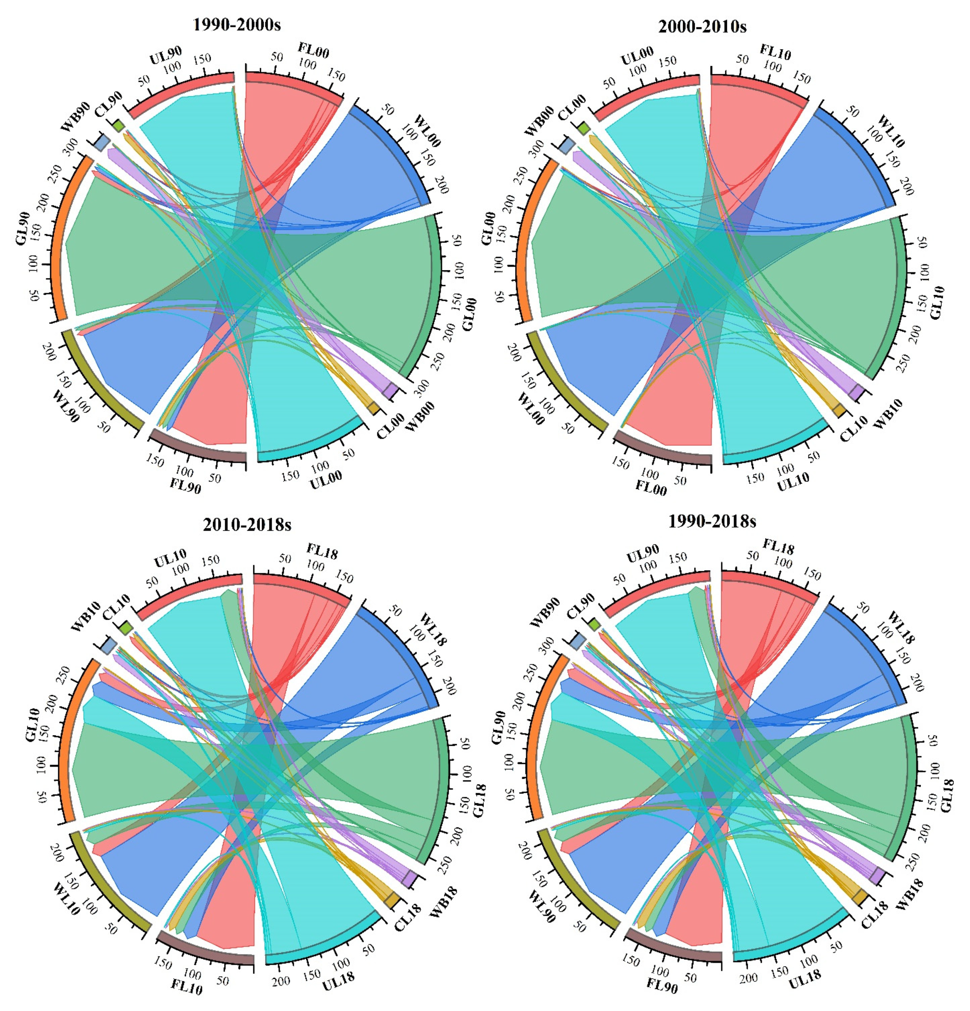
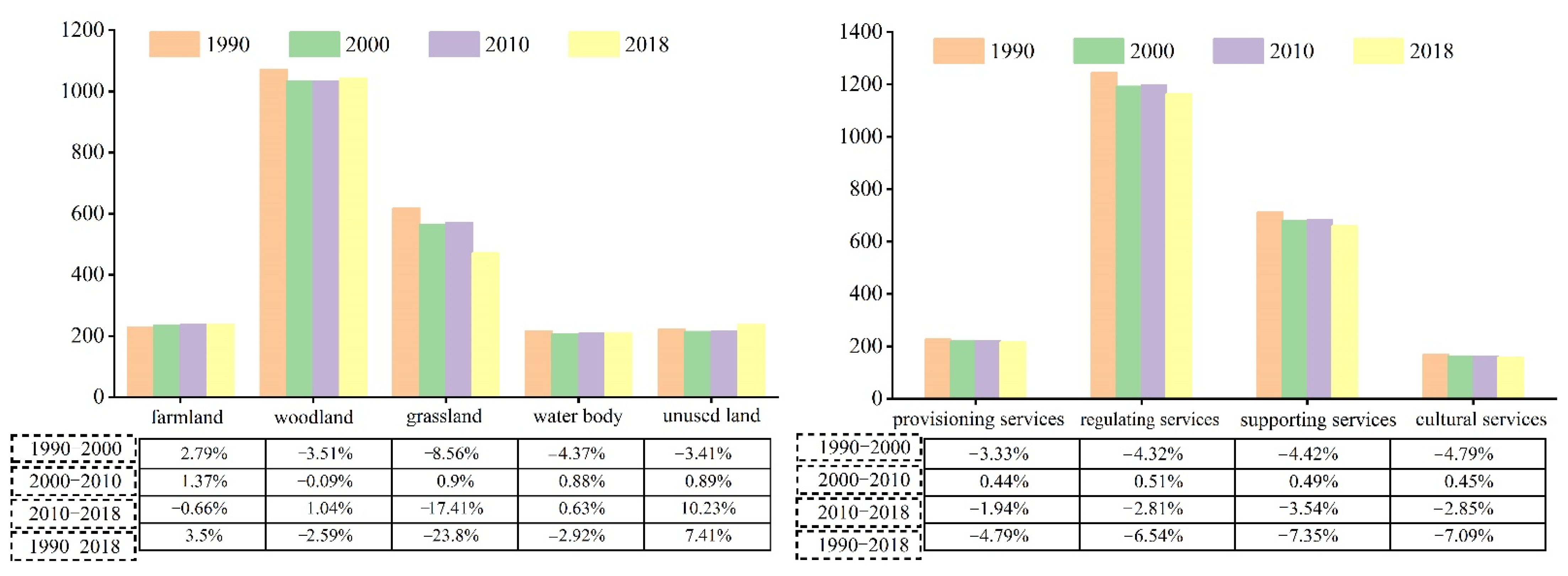
3.1. Change in Land Use from 1990 to 2018
3.2. Spatiotemporal Variation of ESV
3.2.1. Spatiotemporal Variation of ESV from 1990 to 2018
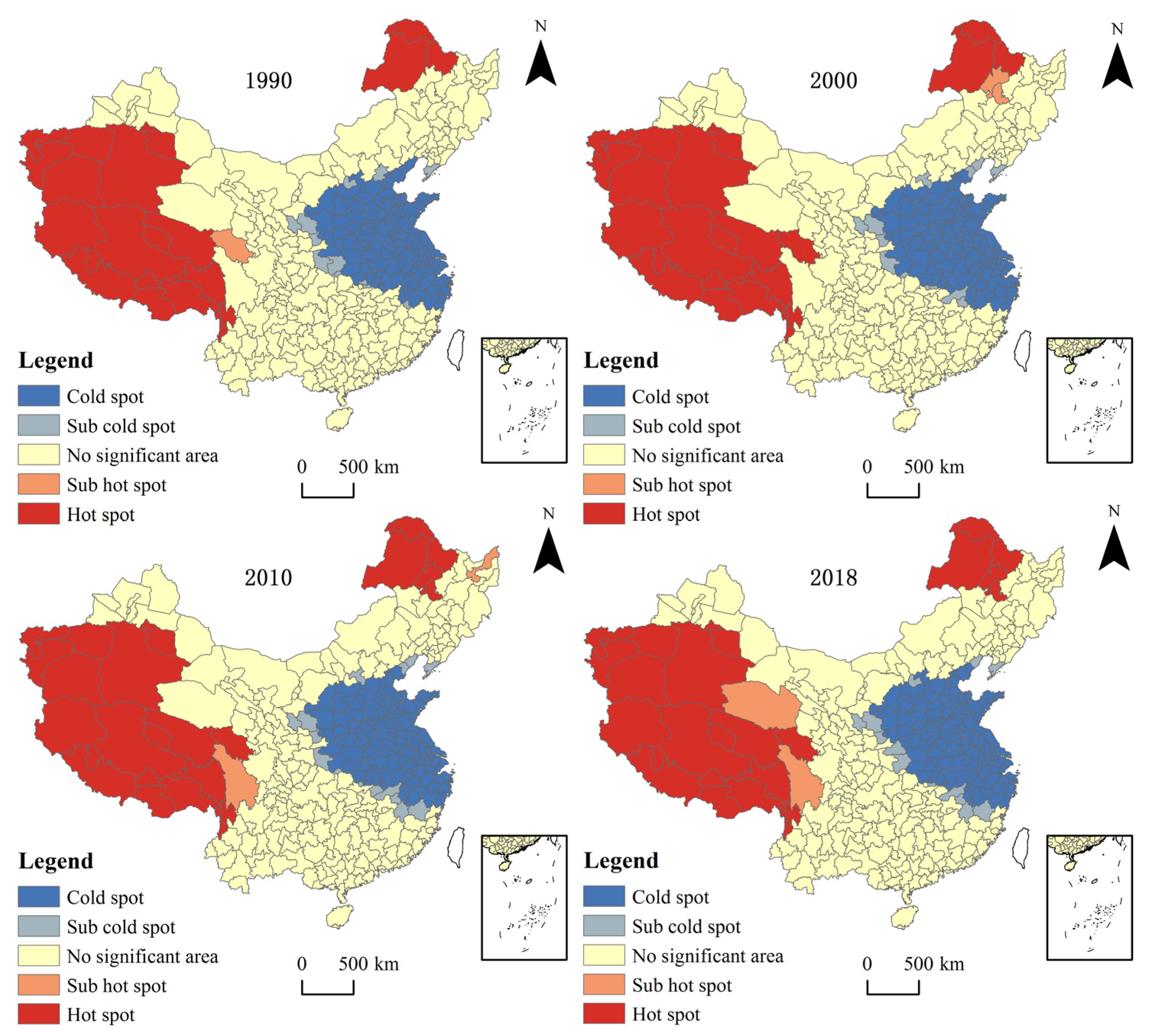
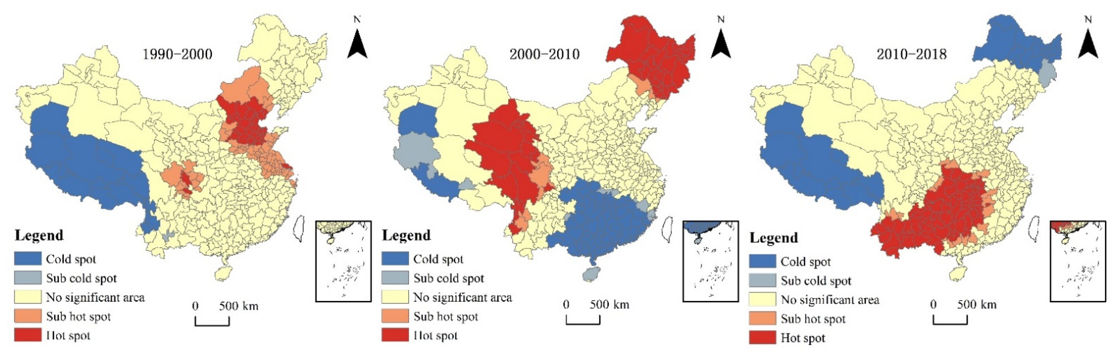
3.2.2. Evolution Characteristics of Cold and Hot Spots of Ecosystem Service Value
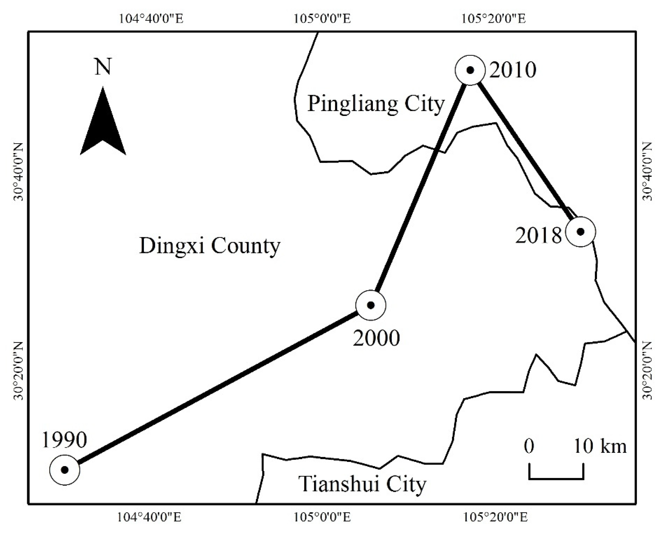
3.2.3. Barycenter Evolution of Ecosystem Service Value
3.3. Driving Factors of Regional Differences in Ecosystem Service Value
4. Discussion
4.1. ESV Dynamic Change in Response to LUCC in China
4.2. Impact Factors on ESV Distribution
4.3. Limitations and Improvement
5. Conclusions
Author Contributions
Funding
Institutional Review Board Statement
Informed Consent Statement
Data Availability Statement
Conflicts of Interest
References
- De Groot, R.S.; Wilson, M.A.; Boumans, R.M. A typology for the classification, description and valuation of ecosystem functions, goods and services. Ecol. Econ. 2002, 41, 393–408. [Google Scholar] [CrossRef] [Green Version]
- Costanza, R. Ecosystem services in theory and practice. Encycl. Anthr. 2018, 3, 419–422. [Google Scholar]
- Small, N.; Munday, M.; Durance, I. The challenge of valuing ecosystem services that have no material benefits. Glob. Environ. Chang. 2017, 44, 57–67. [Google Scholar] [CrossRef]
- Liu, Z.; Wu, R.; Chen, Y.; Fang, C.; Wang, S. Factors of ecosystem service values in a fast-developing region in China: Insights from the joint impacts of human activities and natural conditions. J. Clean. Prod. 2021, 297, 126588. [Google Scholar] [CrossRef]
- Hauck, J.; Görg, C.; Varjopuro, R.; Ratamäki, O.; Maes, J.; Wittmer, H.; Jax, K. “Maps have an air of authority”: Potential benefits and challenges of ecosystem service maps at different levels of decision making. Ecosyst. Serv. 2013, 4, 25–32. [Google Scholar] [CrossRef]
- Costanza, R.; d’Arge, R.; De Groot, R.; Farber, S.; Grasso, M.; Hannon, B.; Limburg, K.; Naeem, S.; Paruelo, J.; Van Den Belt, M.; et al. The value of the world’s ecosystem services and natural capital. Nature 1997, 387, 253–260. [Google Scholar] [CrossRef]
- Li, W.; Wang, L.; Yang, X.; Liang, T.; Zhang, Q.; Liao, X.; White, J.R.; Rinklebe, J. Interactive influences of meteorological and socioeconomic factors on ecosystem service values in a river basin with different geomorphic features. Sci. Total Environ. 2022, 829, 154595. [Google Scholar] [CrossRef]
- Wang, A.; Liao, X.; Tong, Z.; Du, W.; Zhang, J.; Liu, X.; Liu, M. Spatial-temporal dynamic evaluation of the ecosystem service value from the perspective of “production-living-ecological” spaces: A case study in Dongliao River Basin, China. J. Clean. Prod. 2022, 333, 130218. [Google Scholar] [CrossRef]
- Pan, N.; Guan, Q.; Wang, Q.; Sun, Y.; Li, H.; Ma, Y. Spatial differentiation and driving mechanisms in ecosystem service value of arid region: A case study in the middle and lower reaches of Shule River Basin, NW China. J. Clean. Prod. 2021, 319, 128718. [Google Scholar] [CrossRef]
- De Groot, R.; Brander, L.; Van Der Ploeg, S.; Costanza, R.; Bernard, F.; Braat, L.; Christie, M.; Crossman, N.; Ghermandi, A.; van Beukering, P.; et al. Global estimates of the value of ecosystems and their services in monetary units. Ecosyst. Serv. 2012, 1, 50–61. [Google Scholar] [CrossRef]
- Xie, G.; Zhen, L.; Lu, C.; Xiao, Y.; Chen, C. Expert Knowledge Based Valuation Method of Ecosystem Services in China. J. Nat. Resour. 2008, 23, 911–919. [Google Scholar]
- Maimaiti, B.; Chen, S.; Kasimu, A.; Simayi, Z.; Aierken, N. Urban spatial expansion and its impacts on ecosystem service value of typical oasis cities around Tarim Basin, northwest China. Int. J. Appl. Earth Obs. Geoinf. 2021, 104, 102554. [Google Scholar] [CrossRef]
- Song, F.; Su, F.; Mi, C.; Sun, D. Analysis of driving forces on wetland ecosystem services value change: A case in Northeast China. Sci. Total Environ. 2021, 751, 141778. [Google Scholar] [CrossRef]
- Bernués, A.; Tello-García, E.; Rodríguez-Ortega, T.; Ripoll-Bosch, R.; Casasús, I. Agricultural practices, ecosystem services and sustainability in High Nature Value farmland: Unraveling the perceptions of farmers and nonfarmers. Land Use Policy 2016, 59, 130–142. [Google Scholar] [CrossRef]
- Ma, X.; Zhu, J.; Zhang, H.; Yan, W.; Zhao, C. Trade-offs and synergies in ecosystem service values of inland lake wetlands in Central Asia under land use/cover change: A case study on Ebinur Lake, China. Glob. Ecol. Conserv. 2020, 24, e01253. [Google Scholar] [CrossRef]
- Jing, Y.; Chang, Y.; Cheng, X.; Wang, D. Land-use changes and ecosystem services under different sce-narios in Nansi Lake Basin, China. Environ. Monit. Assess. 2021, 193, 21. [Google Scholar] [CrossRef]
- Munang, R.; Thiaw, I.; Alverson, K.; Liu, J.; Han, Z. The role of ecosystem services in climate change adaptation and disaster risk reduction. Curr. Opin. Environ. Sustain. 2013, 5, 47–52. [Google Scholar] [CrossRef]
- Fang, L.; Wang, L.; Chen, W.; Sun, J.; Cao, Q.; Wang, S.; Wang, L. Identifying the impacts of natural and human factors on ecosystem service in the Yangtze and Yellow River Basins. J. Clean. Prod. 2021, 314, 127995. [Google Scholar] [CrossRef]
- Chen, M.; Lu, Y.; Ling, L.; Wan, Y.; Luo, Z.; Huang, H. Drivers of changes in ecosystem service values in Ganjiang upstream watershed. Land Use Policy 2015, 47, 247–252. [Google Scholar] [CrossRef]
- Li, G.; Fang, C.; Wang, S. Exploring spatiotemporal changes in ecosystem-service values and hotspots in china. Sci. Total Environ. 2016, 545, 609–620. [Google Scholar] [CrossRef]
- Bai, L.; Jiang, L.; Yang, D.Y.; Liu, Y.B. Quantifying the spatial heterogeneity influences of natural and socioeconomic factors and their interactions on air pollution using the geographical detector method: A case study of the Yangtze River Economic Belt, China. J. Clean. Prod. 2019, 232, 692–704. [Google Scholar] [CrossRef]
- Liu, X.; Wang, H.; Wang, X.; Bai, M.; He, D. Driving factors and their interactions of carabid beetle distribution based on the geographical detector method. Ecol. Indic. 2021, 133, 108393. [Google Scholar] [CrossRef]
- Wu, C.; Chen, B.; Huang, X.; Wei, Y.D. Effect of land-use change and optimization on the ecosystem service values of Jiangsu province, China. Ecol. Indic. 2020, 117, 106507. [Google Scholar] [CrossRef]
- Li, X.; Guo, J.; Qi, S. Forestland landscape change induced spatiotemporal dynamics of subtropical urban forest ecosystem services value in forested region of China: A case of Hangzhou city. Environ. Res. 2021, 193, 110618. [Google Scholar] [CrossRef] [PubMed]
- Ouyang, X.; Tang, L.; Wei, X.; Li, Y. Spatial interaction between urbanization and ecosystem services in Chinese urban agglomerations. Land Use Policy 2021, 109, 105587. [Google Scholar] [CrossRef]
- Ghebrezgabher, M.G.; Yang, T.; Yang, X.; Sereke, T.E. Assessment of NDVI variations in responses to climate change in the Horn of Africa. Egypt. J. Remote Sens. Space Sci. 2020, 23, 249–261. [Google Scholar] [CrossRef]
- Schindler, K.; Papasaika-Hanusch, H.; Schütz, S.; Baltsavias, E. Improving wide-area DEMs through data fusion-chances and limits. Proc. Photogramm. Week 2011, 11, 159–170. [Google Scholar]
- Redo, D.J.; Aide, T.M.; Clark, M.L.; Andrade-Núñez, M.J. Impacts of internal and external policies on land change in Uruguay, 2001–2009. Environ. Conserv. 2012, 39, 122–131. [Google Scholar] [CrossRef]
- Hou, L.; Wu, F.; Xie, X. The spatial characteristics and relationships between landscape pattern and ecosystem service value along an urban-rural gradient in Xi’an city, China. Ecol. Indic. 2020, 108, 105720. [Google Scholar] [CrossRef]
- Dong, M.; Yang, L.; Su, L.; Chang, L.; Gao, D.; Zhou, J. Study on the value and sensitivity of ecosystem services based on land use change: A case study of Daqing City. J. Saf. Environ. 2014, 14, 330–333. [Google Scholar]
- Yue, J.; Xue, L. Study on the dynamics of land use and ecosystem services value in Shannxi Province. J. China Agric. Univ. 2020, 25, 20–30. [Google Scholar]
- Han, R.; Feng, C.C.; Xu, N.; Guo, L. Spatial heterogeneous relationship between ecosystem services and human disturbances: A case study in Chuandong, China. Sci. Total Environ. 2020, 721, 137818. [Google Scholar] [CrossRef] [PubMed]
- Getis, A.; Ord, J.K. The analysis of spatial association by use of distance statistics. Geogr. Anal. 1992, 24, 189–206. [Google Scholar] [CrossRef]
- Su, L.; Ji, X. Spatial-temporal differences and evolution of eco-efficiency in China’s forest park. Urban For. Urban Green. 2021, 57, 12689. [Google Scholar] [CrossRef]
- Wang, J.F.; Zhang, T.L.; Fu, B.J. A measure of spatial stratified heterogeneity. Ecol. Indicat. 2016, 67, 250–256. [Google Scholar] [CrossRef]
- Zhang, N.; Jing, Y.C.; Liu, C.Y.; Li, Y.; Shen, J. A cellular automaton model for grasshopper population dynamics in Inner Mongolia steppe habitats. Ecol. Model. 2016, 329, 5–17. [Google Scholar] [CrossRef]
- He, J.; Pan, Z.; Liu, D.; Guo, X. Exploring the regional differences of ecosystem health and its driving factors in China. Sci. Total Environ. 2019, 673, 553–564. [Google Scholar] [CrossRef]
- Yi, H.; Güneralp, B.; Filippi, A.M.; Kreuter, U.P.; Güneralp, İ. Impacts of land change on ecosystem services in the San Antonio River Basin, Texas, from 1984 to 2010. Ecol. Econ. 2017, 135, 125–135. [Google Scholar] [CrossRef]
- Zhang, Z.; Xia, F.; Yang, D.; Huo, J.; Wang, G.; Chen, H. Spatiotemporal characteristics in ecosystem service value and its interaction with human activities in Xinjiang, China. Ecol. Indic. 2020, 110, 105826. [Google Scholar] [CrossRef]
- Hu, X.; Hong, W.; Qiu, R.; Hong, T.; Chen, C.; Wu, C. Geographic variations of ecosystem service intensity in Fuzhou City, China. Sci. Total Environ. 2015, 512, 215–226. [Google Scholar] [CrossRef]
- Ma, L.; Cheng, W.; Bo, J.; Li, X.; Gu, Y. Spatio-temporal variation of land-use intensity from a multi-perspective—Taking the middle and lower reaches of Shule River Basin in China as an example. Sustainability 2018, 10, 771. [Google Scholar] [CrossRef] [Green Version]
- Jiang, C.; Wang, F.; Zhang, H.; Dong, X. Quantifying changes in multiple ecosystem services during 2000–2012 on the Loess Plateau, China, as a result of climate variability and ecological restoration. Ecol. Eng. 2016, 97, 258–271. [Google Scholar] [CrossRef]
- Wu, D.; Zou, C.; Cao, W.; Xiao, T.; Gong, G. Ecosystem services changes between 2000 and 2015 in the Loess Plateau, China: A response to ecological restoration. PLoS ONE 2019, 14, e0209483. [Google Scholar] [CrossRef] [Green Version]
- Song, W.; Deng, X. Land-use/land-cover change and ecosystem service provision in China. Sci. Total Environ. 2017, 576, 705–719. [Google Scholar] [CrossRef] [PubMed]
- Zhang, F.; Yushanjiang, A.; Jing, Y. Assessing and predicting changes of the ecosystem service values based on land use/cover change in Ebinur Lake Wetland National Nature Reserve, Xinjiang, China. Sci. Total Environ. 2019, 656, 1133–1144. [Google Scholar] [CrossRef]


| Area | 1990–2018 Average Annual Grain Yield per Unit Area | Area | 1990–2018 Average Annual Grain Yield per Unit Area | Area | 1990–2018 Average Annual Grain Yield per Unit Area | Area | 1990–2018 Average Annual Grain Yield per Unit Area |
|---|---|---|---|---|---|---|---|
| Beijing | 5497.64 | Shanghai | 6491.62 | Hubei | 5655.65 | Yunnan | 3953.27 |
| Tianjing | 4867.92 | Jiangsu | 6116.74 | Hunan | 6003.43 | Xizang | 4668.72 |
| Hebei | 4788.63 | Zhejiang | 6077.69 | Guangdong | 5437.98 | Shaanxi | 3449.46 |
| Shanxi | 3419.26 | Anhui | 5035.62 | Guangxi | 4708.75 | Gansu | 3352.8 |
| Neimenggu | 3948.88 | Fujian | 5332.2 | Hainan | 4155.37 | Qinghai | 3288.11 |
| Liaoming | 5272.28 | Jiangxi | 5310.57 | Chongqing | 5386.97 | Ningxia | 4404.3 |
| Jilin | 6290.21 | Shandong | 5447.66 | Sichuan | 5520.88 | Xinjiang | 5699.57 |
| Heilongjiang | 4685.64 | Henan | 5303.36 | Guizhou | 3948.57 |
| Type | Sub-Type | Farmland | Woodland | Grassland | Water Body | Unused Land | Construction Land |
|---|---|---|---|---|---|---|---|
| Provisioning services | Food production | 1.00 | 0.33 | 0.43 | 0.53 | 0.23 | 0.00 |
| Raw material | 0.39 | 2.98 | 0.36 | 0.35 | 0.20 | 0.00 | |
| Regulating services | Gas regulation | 0.72 | 4.32 | 1.50 | 0.51 | 0.78 | 0.00 |
| Climate regulation | 0.97 | 4.07 | 1.56 | 2.06 | 0.85 | 0.00 | |
| Hydrology regulation | 0.77 | 4.09 | 1.52 | 18.77 | 0.80 | 0.00 | |
| Waste treatment | 1.39 | 1.72 | 1.32 | 14.85 | 0.79 | 0.00 | |
| Supporting services | Soil conservation | 1.47 | 4.02 | 2.24 | 0.41 | 1.21 | 0.00 |
| Biodiversity maintenance | 1.02 | 4.51 | 1.87 | 3.43 | 1.14 | 0.00 | |
| Cluture service | Esthetic landscape provision | 0.17 | 2.08 | 0.87 | 4.44 | 0.56 | 0.00 |
| Total | 7.90 | 28.12 | 11.67 | 45.35 | 6.53 | 0.00 |
| Farmland | Woodland | Grassland | Water Body | Construction Land | Unused Land | |
|---|---|---|---|---|---|---|
| 1990–2000 | 2.89 | −1.18 | −3.34 | 0.27 | 1.38 | −0.04 |
| 2000–2010 | −0.50 | 1.30 | −0.42 | 1.37 | 2.83 | −0.07 |
| 2010–2018 | −0.90 | 2.21 | −34.97 | 0.43 | 6.51 | 22.20 |
| Net change | 1.50 | 2.33 | −38.74 | 2.06 | 10.72 | 22.10 |
| in 1990–2018 |
| Single Land Use Change/% | Comprehensive Land Use Change | ||||||
|---|---|---|---|---|---|---|---|
| Farmland | Woodland | Grassland | Water Body | Construction Land | Unused Land | ||
| 1990–2000 | 0.16 | −0.05 | −0.11 | 0.11 | 0.90 | −0.002 | 0.05 |
| 2000–2010 | −0.03 | 0.06 | −0.01 | 0.53 | 1.69 | −0.003 | 0.03 |
| 2010–2018 | −0.05 | 0.10 | −1.17 | 0.16 | 3.33 | 1.11 | 0.36 |
| 1990–2018 | 0.03 | 0.04 | −0.46 | 0.29 | 2.50 | 0.40 | 0.41 |
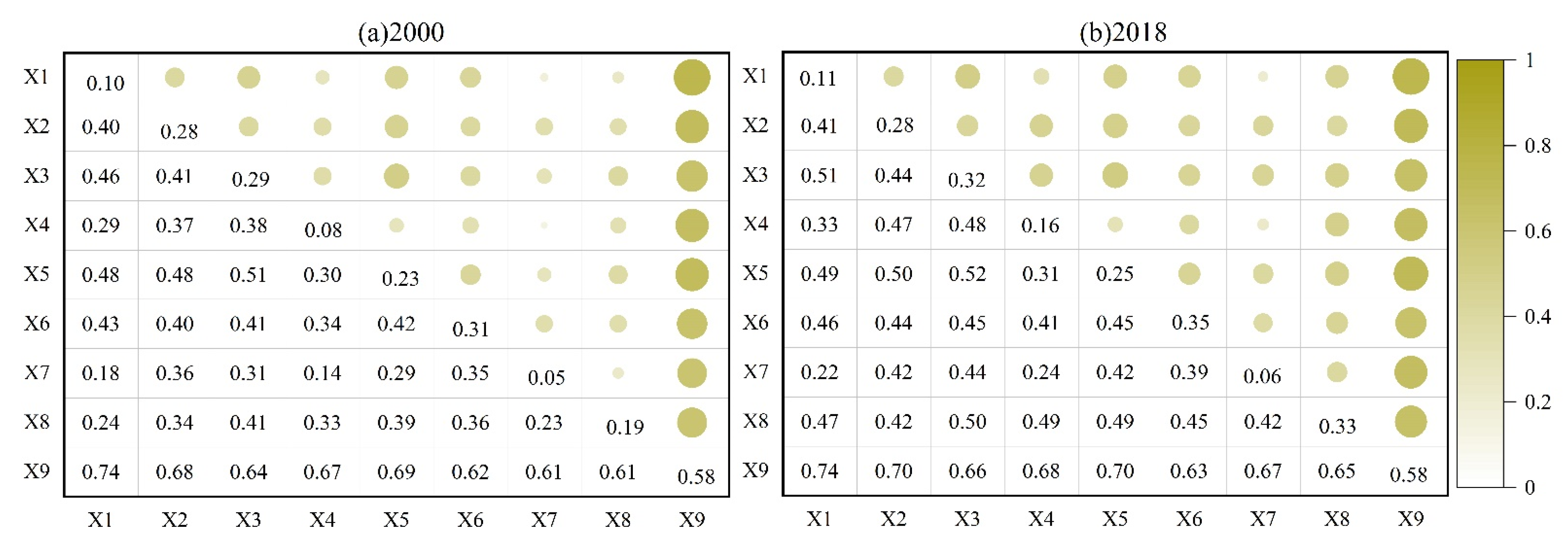
| X1 | X2 | X3 | X4 | X5 | X6 | X7 | X8 | X9 | ||
|---|---|---|---|---|---|---|---|---|---|---|
| Nation | 2000 | 0.10 ** | 0.28 ** | 0.29 ** | 0.08 ** | 0.23 ** | 0.31 ** | 0.05 ** | 0.19 ** | 0.58 ** |
| 2018 | 0.11 ** | 0.28 ** | 0.32 ** | 0.16 ** | 0.25 ** | 0.35 ** | 0.06 ** | 0.33 ** | 0.58 ** | |
| Northeastern region | 2000 | 0.16 | 0.35 | 0.48 * | 0.01 | 0.22 * | 0.33 * | 0.01 | 0.43 ** | 0.41 * |
| 2018 | 0.18 | 0.38 | 0.34 | 0.01 | 0.12 | 0.36 ** | 0.05 | 0.46 * | 0.38 * | |
| North China | 2000 | 0.07 | 0.11 | 0.74 ** | 0.04 | 0.12 | 0.4 ** | 0.08 | 0.44 ** | 0.73 ** |
| 2018 | 0.07 | 0.11 | 0.74 ** | 0.1 | 0.13 | 0.45 ** | 0.13 | 0.79 ** | 0.73 ** | |
| East China | 2000 | 0.46 ** | 0.26 * | 0.04 | 0.44 ** | 0.15 ** | 0.48 ** | 0.04 | 0.48 ** | 0.02 |
| 2018 | 0.44 ** | 0.22 | 0.03 | 0.39 ** | 0.4 ** | 0.44 ** | 0.09 | 0.61 ** | 0.02 | |
| South central region | 2000 | 0.43 ** | 0.41 ** | 0.07 | 0.18 ** | 0.2 ** | 0.55 ** | 0.02 | 0.57 ** | 0.04 |
| 2018 | 0.43 ** | 0.44 ** | 0.02 | 0.22 ** | 0.49 ** | 0.51 ** | 0.08 | 0.62 ** | 0.05 | |
| Northwest region | 2000 | 0.18 | 0.06 | 0.08 | 0.13 * | 0.26 * | 0.21 ** | 0.07 | 0.16 * | 0.57 ** |
| 2018 | 0.19 | 0.07 | 0.13 | 0.24 ** | 0.36 ** | 0.23 ** | 0.09 | 0.26 ** | 0.61 ** | |
| Southwestern region | 2000 | 0.1 | 0.58 ** | 0.65 ** | 0.52 * | 0.76 ** | 0.39 ** | 0.19 | 0.03 | 0.87 ** |
| 2018 | 0.11 | 0.57 ** | 0.65 ** | 0.51 * | 0.67 ** | 0.42 ** | 0.51 ** | 0.16 * | 0.81 ** | |
| Dominant | Dominant | Dominant | ||
|---|---|---|---|---|
| Interaction 1 | Interaction 2 | Interaction 3 | ||
| Northeastern region | 2000 | X2 ∩ X9 (0.855) | X7 ∩ X9 (0.825) | X8 ∩ X9 (0.786) |
| 2018 | X2 ∩ X9 (0.858) | X7 ∩ X9 (0.849) | X2 ∩ X7 (0.746) | |
| North China | 2000 | X5 ∩ X8 (0.954) | X5 ∩ X9 (0.935) | X3 ∩ X9 (0.927) |
| 2018 | X3 ∩ X8 (0.989) | X5 ∩ X8 (0.984) | X2 ∩ X8 (0.983) | |
| East China | 2000 | X1 ∩ X8 (0.667) | X4 ∩ X6 (0.665) | X1 ∩ X4 (0.660) |
| 2018 | X7 ∩ X8 (0.732) | X1 ∩ X8 (0.690) | X4 ∩ X8 (0.661) | |
| South central region | 2000 | X1 ∩ X8 (0.694) | X2 ∩ X8 (0.684) | X1 ∩ X5 (0.679) |
| 2018 | X7 ∩ X8 (0.751) | X1 ∩ X8 (0.750) | X3 ∩ X8 (0.736) | |
| Northwest region | 2000 | X2 ∩ X9 (0.865) | X3 ∩ X9 (0.865) | X4 ∩ X9 (0.849) |
| 2018 | X3 ∩ X9 (0.867) | X2 ∩ X9 (0.865) | X5 ∩ X9 (0.858) | |
| Southwestern region | 2000 | X4 ∩ X9 (0.957) | X1 ∩ X9 (0.954) | X5 ∩ X9 (0.925) |
| 2018 | X5 ∩ X9 (0.928) | X1 ∩ X9 (0.924) | X4 ∩ X9 (0.908) | |
Publisher’s Note: MDPI stays neutral with regard to jurisdictional claims in published maps and institutional affiliations. |
© 2022 by the authors. Licensee MDPI, Basel, Switzerland. This article is an open access article distributed under the terms and conditions of the Creative Commons Attribution (CC BY) license (https://creativecommons.org/licenses/by/4.0/).
Share and Cite
Wei, X.; Zhao, L.; Cheng, P.; Xie, M.; Wang, H. Spatial-Temporal Dynamic Evaluation of Ecosystem Service Value and Its Driving Mechanisms in China. Land 2022, 11, 1000. https://doi.org/10.3390/land11071000
Wei X, Zhao L, Cheng P, Xie M, Wang H. Spatial-Temporal Dynamic Evaluation of Ecosystem Service Value and Its Driving Mechanisms in China. Land. 2022; 11(7):1000. https://doi.org/10.3390/land11071000
Chicago/Turabian StyleWei, Xiaojian, Li Zhao, Penggen Cheng, Mingrui Xie, and Huimin Wang. 2022. "Spatial-Temporal Dynamic Evaluation of Ecosystem Service Value and Its Driving Mechanisms in China" Land 11, no. 7: 1000. https://doi.org/10.3390/land11071000
APA StyleWei, X., Zhao, L., Cheng, P., Xie, M., & Wang, H. (2022). Spatial-Temporal Dynamic Evaluation of Ecosystem Service Value and Its Driving Mechanisms in China. Land, 11(7), 1000. https://doi.org/10.3390/land11071000