Abstract
Heavy metal pollution in soil is threatening the ecological environment and human health. However, field measurement of heavy metal content in soil entails significant costs. Therefore, this study explores the estimation method of soil heavy metals based on remote sensing images and machine learning. To accurately estimate the heavy metal content, we propose a hybrid artificial intelligence model integrating least absolute shrinkage and selection operator (LASSO), genetic algorithm (GA) and error back propagation neural network (BPNN), namely the LASSO-GA-BPNN model. Meanwhile, this study compares the accuracy of the LASSO-GA-BPNN model, SVR (Support Vector Regression), RF (Random Forest) and spatial interpolation methods with Huanghua city as an example. Furthermore, the study uses the LASSO-GA-BPNN model to estimate the content of eight heavy metals (including Ni, Pb, Cr, Hg, Cd, As, Cu, and Zn) in Huanghua and visualize the results in high resolution. In addition, we calculate the Nemerow index based on the estimation results. The results denote that, the simultaneous optimization of BPNN by LASSO and GA can greatly improve the estimation accuracy and generalization ability. The LASSO-GA-BPNN model is a more accurate model for the estimate heavy metal content in soil compared to SVR, RF and spatial interpolation. Moreover, the comprehensive pollution level in Huanghua is mainly low pollution. The overall spatial distribution law of each heavy metal content is very similar, and the local spatial distribution of each heavy metal is different. The results are of great significance for soil pollution estimation.
1. Introduction
As an important natural resource, soil is the environmental basis for human survival. However, the risk of soil pollution by heavy metals is increasing with the increase of human activities. Although industry and agriculture play an irreplaceable role in the rapid economic development, intensive industrial and agricultural activities have also resulted in the enrichment of heavy metals in soil [1,2]. Long-term accumulation of heavy metal elements will cause serious damage to the ecological environment. Meanwhile, heavy metals will be enriched into the human body through the food chain, directly endangering human health. In the context of urban expansion and industrial development, attention is being paid to the problem of heavy metal pollution [3,4,5,6]. However, field measurement of heavy metal content in soil entails significant costs. Therefore, accurately estimating the content of heavy metals in soil is essential for soil resource conservation.
To estimate the heavy metal content in soil, spatial interpolation methods have been widely used. It can be divided into deterministic interpolation, radial basis function method [7,8], and geostatistical interpolation [9,10]. For example, Zhang et al. [11] used the ordinary kriging method to estimate the spatial distribution of Cr in industrial areas and assess the risks to human health. Ogunkunle and Fatoba [12] estimated the content of five heavy metals around a large cement plant by using the inverse distance weighting method. Furthermore, whether there is any difference in accuracy between different interpolation methods in the estimation of heavy metal content in soil has attracted the attention of many scholars. For instance, Duan et al. [13] estimated the content of Zn, Pb, Cd, Cr, As and Ni in soil around an electroplating plant. It was found that the estimation accuracy of the ordinary kriging method was higher than that of the inverse distance weighting method in this study area. Fu et al. [14] predicted the content of Pb in soil using ordinary kriging, geographically weighted regression kriging and regression kriging. The results show that the geographically weighted regression kriging method had the highest accuracy.
Nowadays, with the rapid development of artificial intelligence, machine learning models have exhibited good results in prediction. This has made machine learning widely used in various fields [15,16,17]. The advancement of geographic information technology has also led to the application of remote sensing in many disciplines [18,19,20,21]. In the field of environmental science, many scholars have combined spectral data and machine learning methods for the estimation of heavy metal content in soil, such as support vector regression (SVR) [22,23], artificial neural network (ANN) [24,25,26,27], and random forest (RF) [28,29,30]. On the one hand, the high dimension and redundancy characteristics of spectral data for estimation of heavy metal pollution in soil seriously affect the accuracy and stability of the estimation model. Consequently, numerous scholars determine the appropriate characteristic bands for different heavy metals by statistical analysis methods [27,31]. For example, Lamine et al. [32] used the stepwise regression method to select characteristic bands for estimation models of four heavy metals. Liu et al. [33] analyzed the correlation between nine heavy metals and spectral reflectance by Pearson correlation coefficient and established the optimal estimation model. On the other hand, error back propagation neural network (BPNN) is widely used in the estimation of heavy metal content in soil by virtue of its powerful nonlinear predictive capability. For example, Zhao et al. [34] combined BPNN and spectral data to predict the contents of Cd, Hg, As, Pb, Cu, and Zn in soil around Tai Lake in China and found that the estimation accuracy of the BPNN model is higher than that of the partial least square method. Bian et al. [35] used BPNN and spectral data to predict the content of Cu, Sn, Zn and Pb in different types of soils. The results showed that BPNN had a good prediction effect and generalization ability in predicting the content of heavy metals. Notably, some studies have predicted soil properties by comparing geostatistical models and machine learning models. Wang et al. [36] predicted the contents of Ca and Mg in topsoil and subsoil using ordinary kriging, linear mixed model, quantile regression forests, support vector machine, and Cubist regression kriging, respectively.
Nevertheless, the above-mentioned studies have limitations in the estimation models of heavy metal content in soil. Statistical analysis methods used to remove the redundancy of high-dimensional spectral data are unable to examine the nonlinear relationship between spectral data and heavy metal content. Furthermore, BPNN has strong nonlinear prediction functions and is frequently used in the estimation of heavy metal content in soil. However, the algorithm can easily fall into the local optimal solution. The above two aspects will greatly reduce the accuracy and stability of the estimation model. Besides, the existing studies of estimating heavy metal content using remote sensing data ignore the accuracy comparison between machine learning models and spatial interpolation methods.
This study aims to construct a high accuracy estimation model of heavy metal content in soil. We propose a hybrid artificial intelligence model integrating least absolute shrinkage and selection operator (LASSO), genetic algorithm (GA) and BPNN, namely the LASSO-GA-BPNN model. Then, taking Huanghua as an example, this study uses the field sampling data of eight heavy metals, spectral reflectance factors, spectral exponential factors, latitude and longitude, and relief factors to construct the dataset. The eight heavy metals in the dataset include Ni, Pb, Cr, Hg, Cd, As, Cu, and Zn. The dataset is used to train and validate the model. Meanwhile, we compare the accuracy of the LASSO-GA-BPNN model, SVR model, RF model, inverse distance weighting method and ordinary kriging method. Moreover, the study uses the LASSO-GA-BPNN model to estimate the heavy metal content in Huanghua and visualize it with high resolution. Based on this, we calculate the Nemerow index and analyze the spatial distribution of heavy metal pollution in this area.
Our key contributions are twofold. First, this paper constructs a new model for estimating soil heavy metal content, namely the LASSO-GA-BPNN model. The model has high estimation accuracy. Second, in the field of estimating heavy metal content using remote sensing data, this study is the first to compare the estimation accuracy between spatial interpolation methods and machine learning models.
2. Materials and Methods
2.1. Study Area
In this study, Huanghua City is taken as the study area, and the location is shown in Figure 1. Huanghua is located in the east of North China Impact Plain, bordering the Bohai Sea in the east and Tianjin in the north, and its geomorphological types are plain and coastal zone. Heavy metals that cause soil pollution mainly include Ni, Pb, Cr, Hg, Cd, As, Cu and Zn. Therefore, sample data of these eight elements are obtained through field sampling. Field sampling was performed in November 2013. The sampling points are positioned in a uniform arrangement with soil sampling depths of 0 to 20 cm (A few sampling points are located in areas where salt is produced, and some enterprises extract salt through solarization of seawater. Therefore, we sampled in November, when there are no production activities or water at these sites). A total of 516 soil samples are collected, and the latitude and longitude are located by GPS. In addition, we use the Nemerow index as the comprehensive pollution index, and its calculation method is shown in Equations (1) and (2) [37,38]. is the Nemerow index. less than 1 represents no pollution, higher than 1 is less than or equal to 2 represents low pollution, higher than 2 is less than 3 represents moderate pollution, higher than 3 represents high pollution.
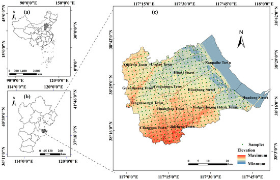
Figure 1.
Location of Huanghua City (c) in Hebei Province (b), China (a).
In Equations (1) and (2), is the single-factor pollution evaluation index of heavy metal , is the measured value, is the evaluation standard, is the average value of , and is the maximum value of , is the Nemerow index. We choose the background value of soil heavy metals in Hebei Province as the evaluation standard.
Shuttle Radar Topography Mission (SRTM) imagery and Landsat 8 Operational Land Imager (OLI) imagery are downloaded from US Geological Survey, https://earthexplorer.usgs.gov/ (accessed on 1 May 2022). OLI imagery was taken on 29 November 2013. We pre-process the OLI imagery with radiation calibration and atmospheric correction, and multi-spectral data is extracted after clipping. Based on this, basic information of the spectral reflectance factors and spectral exponential factors are shown in Table A1 and Table A2. Relief factors including elevation, slope and aspect are extracted from SRTM imagery. According to scorpan model, the content of heavy metals in soil is closely related to soil, climate, organisms, topography, parent materials, age, and space [39,40]. Therefore, field sampling data of eight heavy metals, spectral reflectance factors, spectral exponential factors, latitude and longitude, and relief factors are used to construct the dataset. The dataset is used to train and validate the model. In the construction of the machine learning model, we divide the dataset into the training set and testing set according to the principle of 8:2.
2.2. Methods
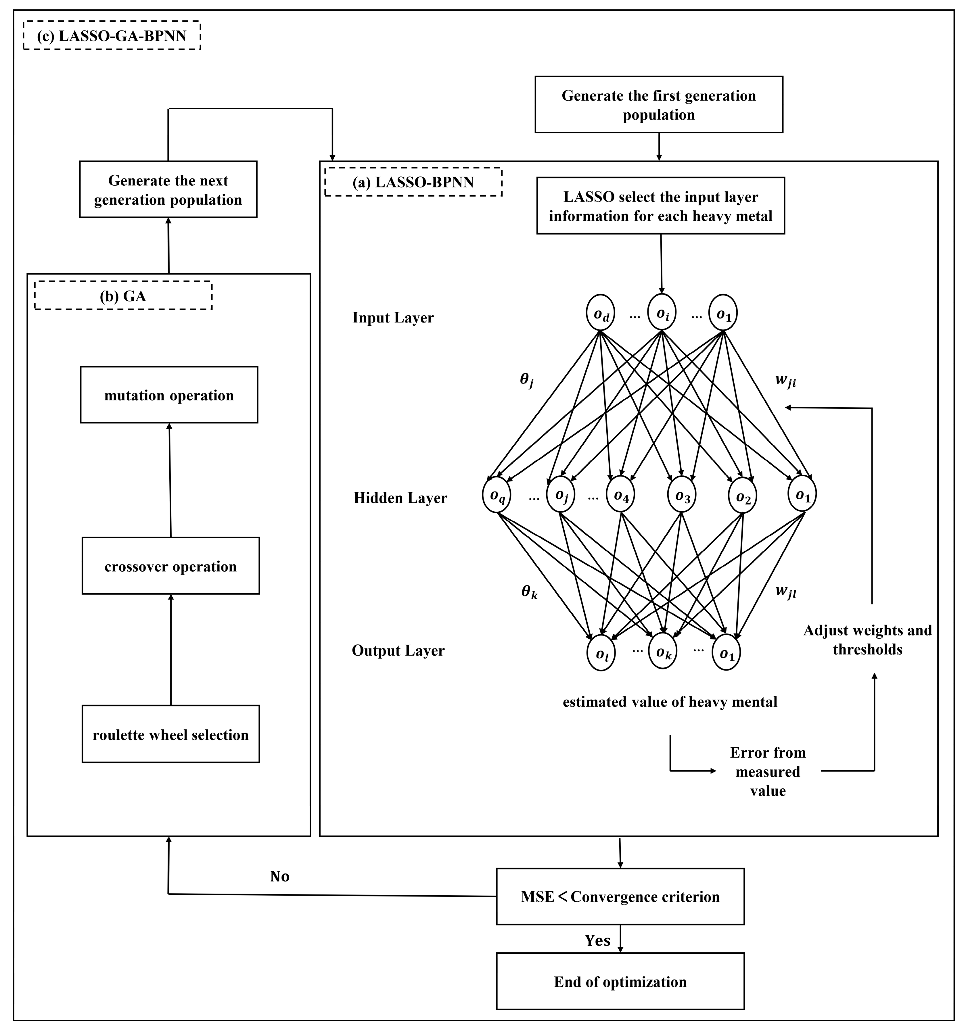
2.2.1. LASSO-GA-BPNN Model
Spectral data used in the field of soil heavy metal pollution estimation has the characteristics of high dimension and high redundancy, which will seriously affect the accuracy and stability of the estimation model. Therefore, this study selects the characteristic bands for each heavy metal. The least absolute shrinkage and selection operator proposed by Tibshirani is a compression estimation method [41], it obtains a better model by constructing a penalty function. This method can compress some regression coefficients to zero, to achieve the effect of subset contraction. Equation (3) is the LASSO estimation of the regression model, where the second term is L1 penalty and is a non-negative regularization parameter. When is zero, LASSO regression is ordinary least square regression. With the increase of , LASSO can compress the coefficients of unimportant variables to 0, realizing the selection of variables. The larger the value of , the more coefficients compressed to 0, the less the complexity of the model and the stronger the explanatory power of the model [41,42,43].
In this study, LASSO and GA are used to optimize BPNN. Specifically, we first select the appropriate input layer information for each heavy metal by LASSO. Then, the weight and threshold of BPNN are optimized by GA. Finally, BPNN is trained, and the LASSO-GA-BPNN model is constructed. The BPNN proposed by Rumelhart is a multilayer feedforward network trained by the error back propagation algorithm, it is suitable for the analysis of various nonlinear relations [44].
The basic structure of the LASSO-BPNN model is shown in Figure 2a, which consists of an input layer, an output layer and several hidden layers. The result of LASSO determines the number of neurons in the input layer in BPNN, and the number of neurons in the hidden layer is determined according to the empirical Equation (4). BPNN repeatedly adjusts the weights and thresholds by the steepest descent method and error back propagation algorithm. BPNN includes two operation processes, the signal forward propagation process and the error backward propagation process. First, input the input layer information to neurons in the input layer, and the output layer information is generated through the signal forward propagation process, and calculate the error with the expected output. Furthermore, the BPNN transmits error to the neurons in the hidden layer through the error back propagation process and adjusts the weights and thresholds according to the error. This iterative process is the operation process of the neural network until the estimated value of the network is as close as possible to the measured value. The hidden layer information is calculated by the Equation (5), and the output layer information is calculated by Equation (6) [45,46].
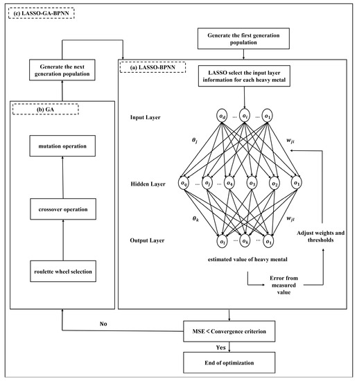
Figure 2.
The basic structure of the LASSO-GA-BPNN model ((a–c) represents the structure of LASSO-BPNN, GA, and LASSO-GA-BPNN, respectively).
In these above three equations, is the number of neurons in the input layer, and is the number of neurons in the hidden layer, is a parameter with a value between 1 and 10, and are activation functions and weight between the input layer and the hidden layer, and are activation functions and weight between the hidden layer and the output layer, is the threshold value of neurons in the input layer, and is the threshold value of neurons in the output layer.
The steepest descent algorithm used in the LASSO-BPNN model is easy to fall into the local optimal solution. Therefore, this study uses GA to optimize the LASSO-BPNN model, and the GA operation flow is shown in Figure 2b. GA is a random search optimization method based on natural genetic mechanisms and biological evolution theory [47,48]. There are no other restrictions on this algorithm, and its solution set is very complete. In the iterative process of GA, the set of existing solutions can always move towards the global optimal solution, which has a strong search purpose. This feature can help the LASSO-BPNN model find the optimal combination of weights and thresholds, and then realize the global optimal solution. The basic structure of the LASSO-GA-BPNN model is shown in Figure 2c [45].
2.2.2. SVR Model
The basic principle of SVR is to use nonlinear mapping to map data to high-dimensional feature space, then construct regression estimation function in high-dimensional feature space, and then map it back to the original space. SVR is a nonlinear algorithm and can effectively avoid the problem of local minima. Let be the independent variable and be the dependent variable. For the training set , its regression function is Equation (7), which is calculated according to the objective Function (8) [49,50,51].
In these above three equations, is the normal vector, is the displacement term, is the regularization parameter, and is relaxation variable. represents the nonlinear transfer function. The epsilon is an insensitive-loss function. A large epsilon means larger errors are admitted and not penalized [52]. The original objective function can be transformed into a dual problem via the Lagrange multiplier method, as shown in Equation (10), where is the kernel function. In this study, the value of epsilon is 0.1 and the kernel function is a Gaussian radial basis function [52].
2.2.3. RF Model
RF is an important model used to predict soil properties, which was proposed by Breiman [53]. Random forest is an ensemble model based on regression tree algorithm, which forms a “forest of models” by constructing many regression trees [52]. Then, these decision trees are integrated using the averaging function. Compared to a single decision tree, random forests are a stable and accurate prediction model. Since each decision tree is trained on a unique subsample of the sample dataset, the random forest avoids overfitting [28,54]. The number of regression trees contained in the RF is n, and the number of variables used in the binomial tree in the nodes is m. They are two important hyper-parameters in the RF. The n decides the trade-off between computational complexity and accuracy of RF [55]. The m decides the strength of an RF model as it decides the strength of every single tree in the forest and the relationship between any two trees. When m is increasing, the strength of the single tree is increasing, while the relationship between any two trees also increases. Single tree strength can improve RF performance, while the high correlation between trees weakens the performance [52,56]. In this study, we optimize the values of n (100–1600) and m (1–12) by the traversal method to improve the prediction ability of RF model.
2.2.4. Inverse Distance Weighting Method
As one of the deterministic interpolation methods, inverse distance weighting is widely used. It estimates by calculating the weighted average of the points in the neighborhood of the target estimated point . The weighting method is the reciprocal of the distance between the point and the point . The estimated value of the point calculated using IDW is calculated by Equation (11) [57,58].
In Equation (11), is the total number of sample points in the neighborhood of the point , is the attribute value at point .
2.2.5. Ordinary Kriging Method
Ordinary kriging is a geostatistical interpolation method. If the data is highly continuous in space, the points closer to the estimated point will get a higher weight than those farther away. The weight is selected according to the minimization of the estimated variance. Therefore, the estimated value of the point obtained by the ordinary kriging method is based on semivariogram theory, and is calculated by the linear combination of sample points within the influence range of the estimated point. The calculation method is Equation (12) [59].
2.2.6. Accuracy Evaluation Index
To test the estimation accuracy of the LASSO-GA-BPNN model, three evaluation indexes are selected. Root mean square error (RMSE) can evaluate the change degree of data and compare models. The result of RMSE is of the same order of magnitude as the sampled data, so it can better describe the data, the smaller RMSE, the higher the estimation accuracy of the model. Mean Absolute Error (MAE) is the average of the absolute value of the difference between the estimated value and the measured value. The smaller the MAE, the higher the accuracy of the model. Compared with MAE, Mean Absolute Percentage Error (MAPE) increases the denominator under the difference between the estimated value and the measured value, so it can be used to compare the estimation effects under different dimensions. The closer the MAPE is to 0%, the higher the accuracy of the model is. The calculation methods of the above accuracy evaluation indexes are Equations (13)–(15).
In these above three equations, is the sample point, is the measured value of heavy metal content, is the estimated value of heavy metal content, is the number of samples.
3. Results and Discussion
3.1. Statistical Characteristics Analysis of Sampled Data
According to the sampled data in Huanghua, the basic statistical characteristics of eight heavy metals are shown in Table 1. The average content of Pb, Cd and Cu is higher than the background values of Hebei Province, and the over-standard rate exceeded 50%. The over-standard rates of other heavy metals are all above 10%. The variation coefficient of each heavy metal content is in the range of 0.1 to 1, which belongs to medium variation. The variation coefficient of Hg is the largest, which indicates that it has obvious discrete characteristics. The average content of each heavy metal is less than the second-class soil quality standard of China, which shows that the soil quality in Huanghua can maintain human health and agricultural production. However, combined with the statistical analysis of sample sites, it was found that the content of heavy metals in some soils is high.

Table 1.
Statistical characteristics analysis of sample points.
3.2. Model Improvement and Accuracy Comparison
3.2.1. Analysis of LASSO Optimization Results
According to the variable selection results of LASSO, the input layer information of neurons in the input layer of LASSO-GA-BPNN model are shown in Table 2. The x and y represent longitude and latitude, respectively. Therefore, the basic topological structures of the LASSO-GA-BPNN model can be determined according to Table 2. For example, the number of input layer neurons of LASSO-GA-BPNN is ten when estimating the content of Ni in soil. As the spectral data characteristics of each heavy metal in each band are different, the results of spectral reflectance factors and spectral exponential factors of each heavy metal are also different. In general, LASSO realizes dimensionality reduction of high-dimensional data and removes redundant variables for each heavy metal, which is more suitable for machine learning estimation models with nonlinear prediction functions. Therefore, LASSO improves the generalization ability of the LASSO-GA-BPNN model. The result is in line with previous research [60].
Table 2.
The input layer information.
3.2.2. Analysis of GA Optimization Results
In the basic parameters of GA, the population size is 100, the maximum number of evolutions is 100, the crossover probability is 0.7, and the mutation probability is 0.1. This means that the best individual is obtained by breeding a population of 100 individuals for 100 generations, and the crossover probability and mutation probability in each evolution process is 70% and 10%, respectively. RMSE is used as the criterion of individual fitness, the higher the model accuracy, the better the individual is.
According to the empirical equation and the results of the variable selection of LASSO, the number of neurons in the hidden layer ranged from 3 to 12 for Hg, from 5 to 14 for Cd and Zn, and from 4 to 13 for the other five heavy metals. The number of hidden layer neurons in the hidden layer in the LASSO-BPNN model has a great influence on the model effect. Therefore, this study optimizes the LASSO-BPNN model with the number of hidden neurons in the hidden layer by GA, and the number of neurons in the hidden layer with the highest accuracy is selected according to the optimized results. The optimal number of neurons in the hidden layer of each heavy metal and the results of accuracy evaluation indexes before and after optimization are shown in Table 3. After GA optimization, RMSE, MAE and MAPE values of the LASSO-GA-BPNN model of each heavy metal decreased obviously. In addition, the estimation accuracy of BPNN is low compared to that of LASSO-BPNN. Therefore, the estimation accuracy of the LASSO-GA-BPNN model is greatly improved compared with the LASSO-BPNN model and BPNN model.
Table 3.
GA optimization results.
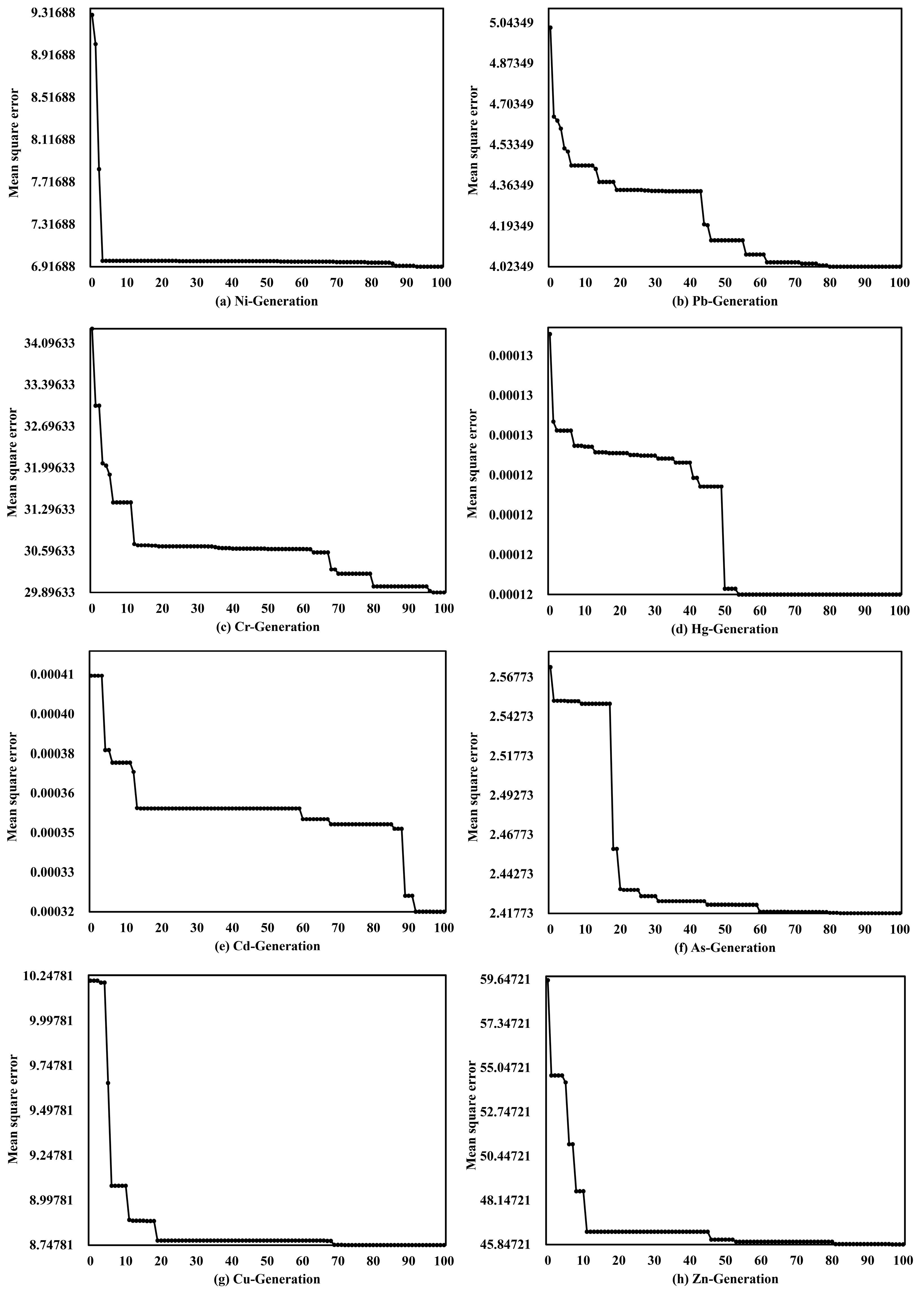
In the LASSO-GA-BPNN model of each heavy metal, the process of GA finding the best weight and threshold is shown in Figure 3a–h. The mean square error is the square of RMSE, which is used as the standard to select the optimal parameters. During the first 20 times of parameter optimization, the mean square error of each heavy metal estimation model decreased obviously. The mean square errors of Pb, Hg, As and Zn tend to be flat after 50 times of parameter optimization. The mean square errors of Cr and Cd tend to be flat after 90 times of parameter optimization. It shows that the LASSO-GA-BPNN model of each heavy metal can converge to the global optimum within 100 times of GA optimization. In general, the optimization process of the LASSO-GA-BPNN model by GA greatly improves the estimation accuracy, which is similar to previous research [45]. It can be judged that the optimization effect of GA is very obvious, which solves the defect that the steepest descent method is easy to fall into the local optimal solution. Therefore, combined with the previous analysis, the simultaneous optimization of BPNN by LASSO and GA can greatly improve the estimation accuracy and generalization ability.
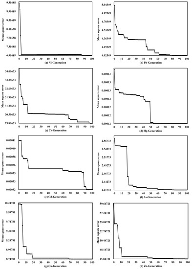
Figure 3.
GA parameter optimization process ((a–h) correspond to the elements of Ni, Pb, Cr, Hg, Cd, As, Cu and Zn, respectively).
3.2.3. Comparison between LASSO-GA-BPNN and SVR and RF
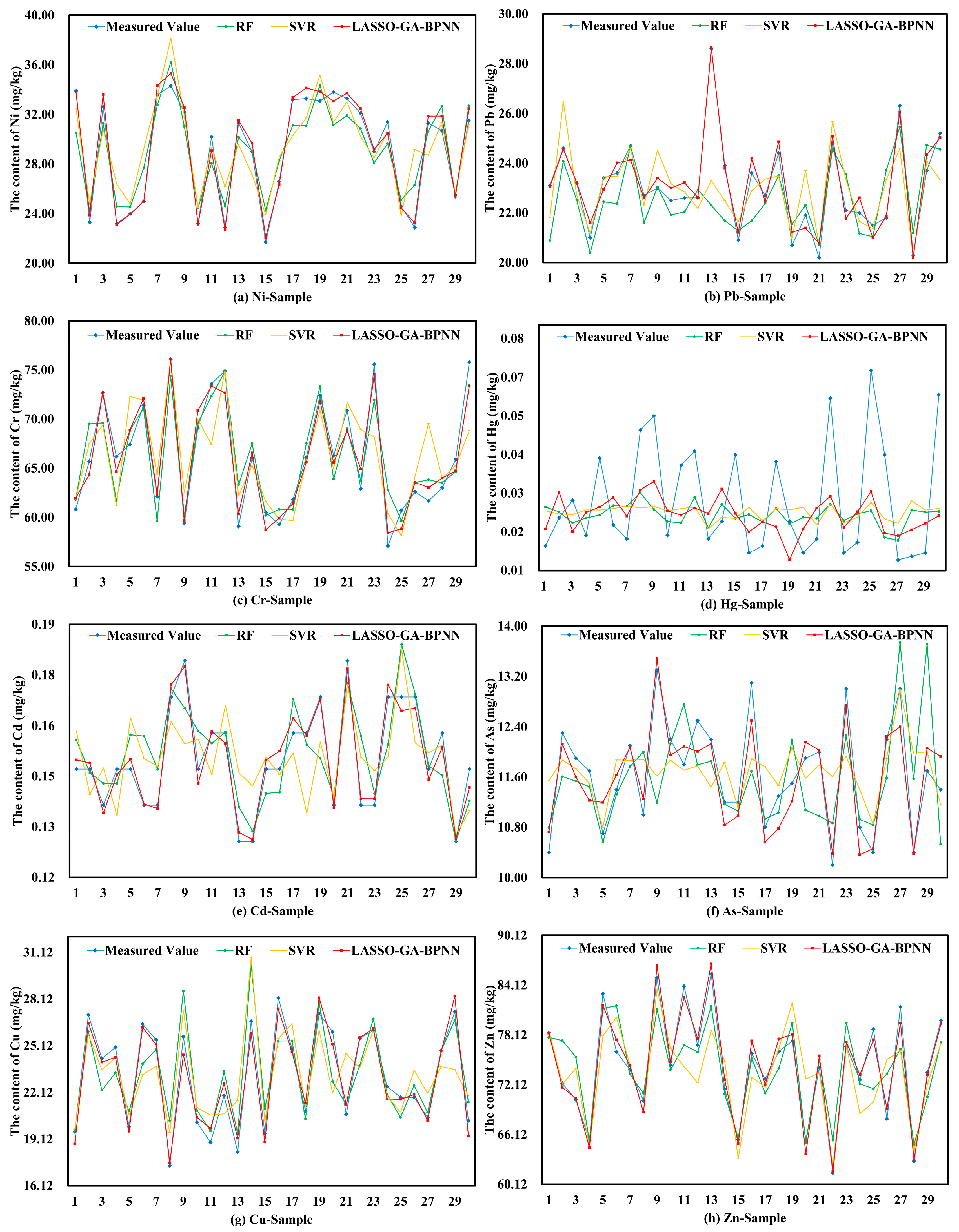
We randomly select 30 samples from the test set for each heavy metal. The fitting effect between the measured value and the estimated value of each heavy metal is shown in Figure 4a–h. There is an obvious gap between the estimated value and the measured value of Hg, and the fitting effect is poor. Besides, the fitting effect of other heavy metals by the three machine learning models is great, and the estimated value of each sample point is close to the measured value. In addition, the LASSO-GA-BPNN model has a better fitting effect than the SVR model and the RF model.
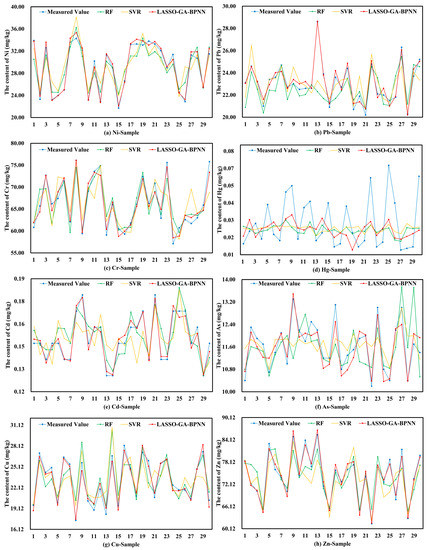
Figure 4.
The estimated value and the measured value of the test set ((a–h) correspond to the elements of Ni, Pb, Cr, Hg, Cd, As, Cu and Zn, respectively; the blue dots are the measured values of every elemental in the soil, and the green, orange, and red dots are the estimated values from the RF, SVR, and LASSO-GA-BPNN models, respectively).
To compare the estimation effects of the three machine learning models, we calculate the accuracy evaluation indexes of each model. The results are shown in Table 4. The MAPE of Hg is 33.0121%, 35.2015%, and 31.4023%, which indicates that the estimation effects of the three machine learning models are poor. The estimation results of the other heavy metals are good, with MAPE below 13%. The RMSE, MAE, and MAPE of each heavy metal in the LASSO-GA-BPNN model are smaller than that of the SVR model and RF model. Therefore, the LASSO-GA-BPNN model has higher estimation accuracy than the SVR model and RF model.
Table 4.
Accuracy evaluation index.
3.2.4. Comparison between LASSO-GA-BPNN and Spatial Interpolation
We compare the accuracy of the LASSO-GA-BPNN model, RF, SVR, inverse distance weighting method and ordinary kriging method, and RMSE is used as the index to examine the accuracy. The RMSE results estimated by each method for each heavy metal are shown in Table 5. Compared with the ordinary kriging method, the RMSE of six heavy metals estimated by the inverse distance weighting method is low. It shows that the overall estimation accuracy of the inverse distance weight method is higher than the ordinary kriging method. Similarly, the RMSE of five heavy metals estimated by RF is low compared to the spatial interpolation methods. In contrast, compared with the spatial interpolation methods, the RMSE of more than half of the heavy metals estimated by SVR is high. Overall, the estimation accuracy of RF is higher than the inverse distance weighting method and ordinary kriging method, while the estimation accuracy of SVR is lower than the two spatial interpolation methods. Furthermore, the RMSE of each heavy metal estimated by the LASSO-GA-BPNN model is smaller than that of the two spatial interpolation methods. This means that the accuracy of LASSO-GA-BPNN is higher than that of inverse distance weighting and ordinary kriging. Consequently, the LASSO-GA-BPNN model is a more accurate model for the estimate heavy metal content in soil compared to SVR, RF and spatial interpolation.
Table 5.
The RMSE of the LASSO-GA-BPNN model and spatial interpolation methods.
3.3. Estimation of Soil Heavy Metal Pollution in Huanghua
3.3.1. Statistical Analysis of Estimated Value
The spectral reflectance factors, spectral exponential factors, latitude and longitude, and relief factors of Huanghua at the scale of 60 m are extracted. We use the LASSO-GA-BPNN model to estimate the content of heavy metals in soil of Huanghua. According to remote sensing images, Huanghua is divided into 685,389 locations. Statistical analysis of the estimated results of each heavy metal content is shown in Table 6. Specifically, in Huanghua, the average content of Zn and Cr is high. The average contents of five heavy metals, Ni, Cr, Hg, As and Zn, are all lower than the background value, while the contents of three heavy metals, Pb, Cd and Cu, are all higher than the background value.
Table 6.
Estimation results of heavy metal content.
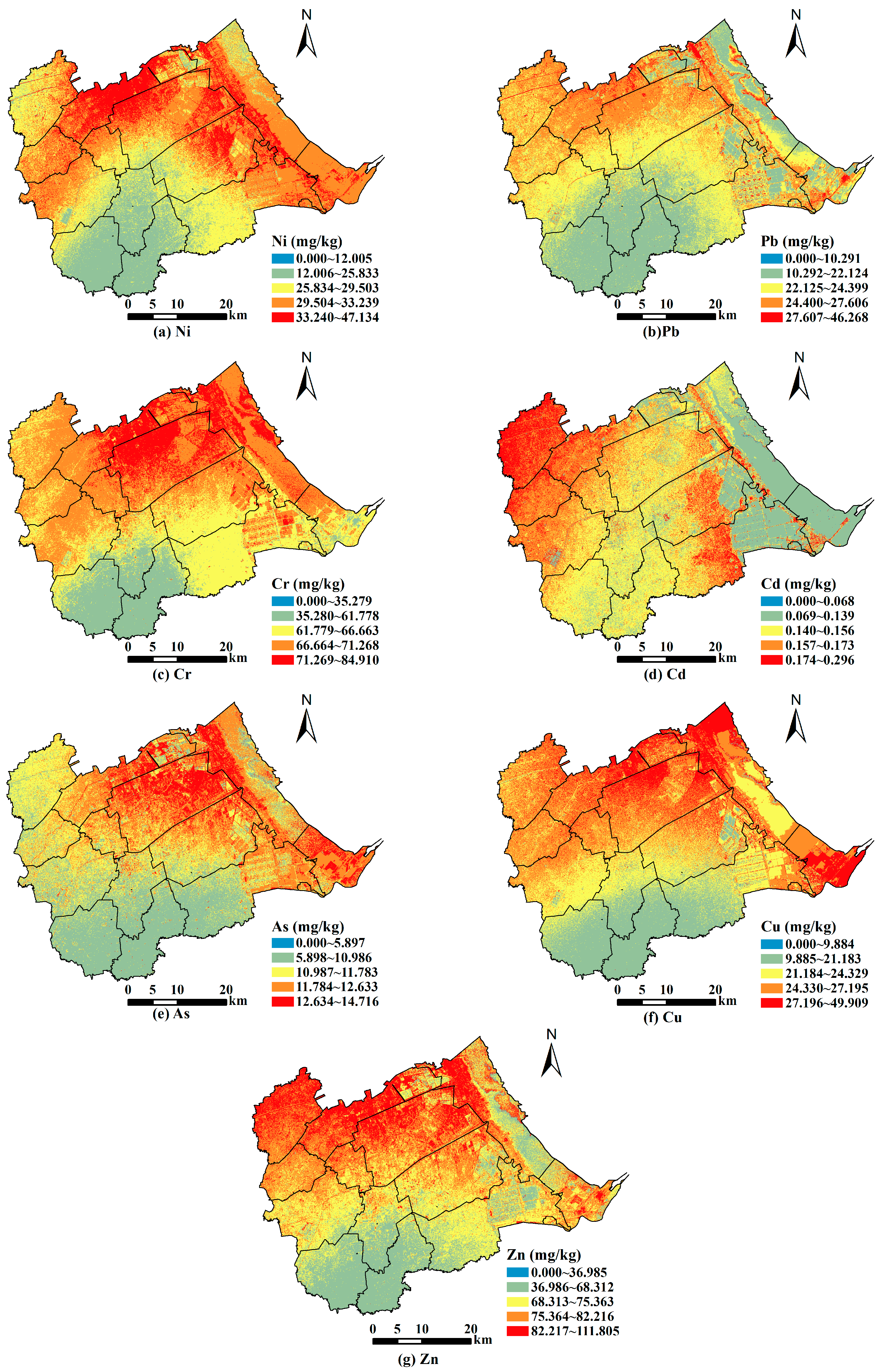
3.3.2. High-Resolution Visualization of the Estimated Value
According to the estimated value of the LASSO-GA-BPNN model for each heavy metal content, we visualize the estimated value with high resolution at the 60 m scale. This can display local spatial distribution in detail and make the results more valuable in the application. We divide the content of each heavy metal into five levels by the natural breakpoint classification method, and the visualization results are shown in Figure 5a–g. Due to the estimation accuracy of Hg element being low, we did not visualize it. Figure 5 shows that the overall spatial distribution law of each heavy metal content is very similar, showing the distribution characteristics of low content in the south, high content in the north, and gradually increasing from south to north. Furthermore, the local spatial distribution of each heavy metal is different. Specifically, the content of each heavy metal in Lvqiao Town is high. Besides, Ni content is high in Huaxi Street and Huazhong Street. Pb content is high in Huaxi Street. Cr content is high in Huaxi Street. Cd content is high in Qijiawu Town, Guanzhuang Town, Huazhong Town and Yangerzhuang Huizu Town. As content is high in some towns such as Huaxi Street and Huazhong Street. Cu content is high in Huaxi Street. The content of Zn is high in Huaxi Street, Guanzhuang Town. Consequently, Lvqiao Town has a high risk of soil contamination by heavy metals.
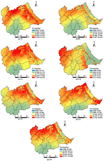
Figure 5.
The spatial distribution of heavy metals in Huanghua ((a–g) correspond to the elements of Ni, Pb, Cr, Cd, As, Cu and Zn, respectively).
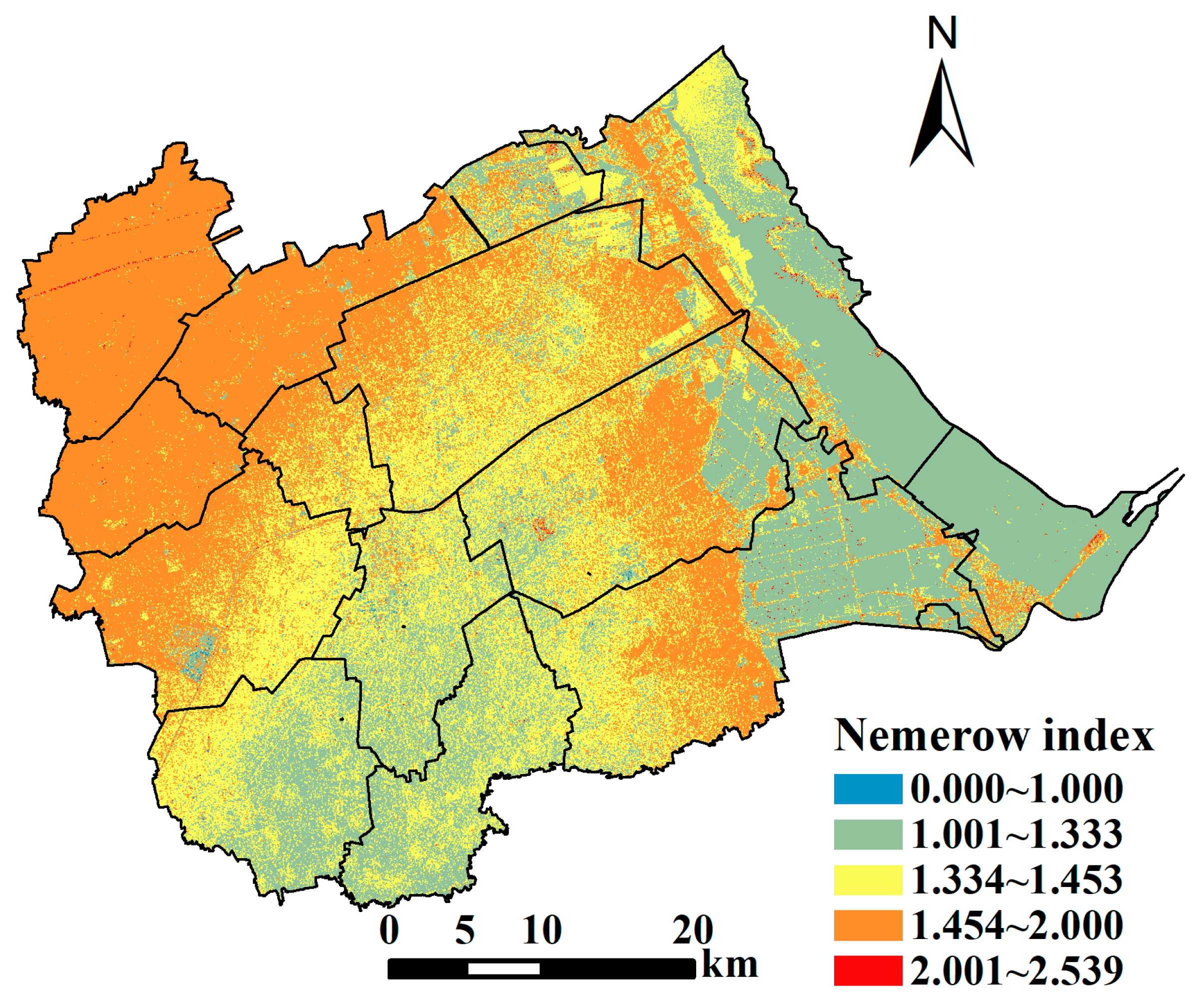
3.3.3. Comprehensive Pollution Index
Nemerow index can reflect the comprehensive pollution level. Therefore, based on the estimated values of the content of seven heavy metals, we calculate the Nemerow index, which is shown in Figure 6. Overall, the spatial distribution law of the comprehensive pollution level of soil heavy metals in Huanghua is very obvious. On the one hand, the values of the Nemerow pollution index are mainly distributed between 1 and 2, with only a few areas having values less than 1 or more than 2. This shows that the comprehensive pollution level of Huanghua is mainly low pollution. On the other hand, on the whole, the pollution level in the southwest and northeast is low, including Changguo Town, Huanghua Town, Jiucheng Town and the eastern part of Huadong Street, Huazhong Street and Yangerzhuang Huizu Town. Additionally, the pollution level in the northwest of Huanghua is high, including Qijiawu Town, Guanzhuang Town and Lvqiao Town.

Figure 6.
The comprehensive pollution index in Huanghua.
First, the comprehensive pollution level in the northwestern part of Huanghua is higher than in other areas, which are the most polluted areas in the city. The reason is that there are chemical and petroleum products and brick manufacturing enterprises in the area. Most of these enterprises are engaged in heavy industry production activities, which often bring high pollution and enrichment of heavy metals to the surrounding land. Meanwhile, there is a large population in this area, and a large number of residents living here for a long time would also cause the enrichment of heavy metals, and compared with industrial production, this factor often causes low pollution to the soil. Besides, two rivers run through the production and residential areas in the middle of Lvqiao Town. This may lead to the large-scale diffusion of heavy metals discharged from industrial production and residential life in the surrounding soil, and indirect enrichment of heavy metals in the surrounding cultivated land. Second, the southwestern part of Huanghua has high elevation and less industrial production activities. Therefore, the comprehensive pollution level of the areas is low. The result is similar to previous research [61].
4. Conclusions
This study proposes a hybrid artificial intelligence model integrating LASSO, GA and BPNN, namely the LASSO-GA-BPNN model. The field sampling data of eight heavy metals, spectral reflectance factors, spectral exponential factors, latitude and longitude, and relief factors are used to construct the dataset. Then, we compare the accuracy of the LASSO-GA-BPNN model, SVR model, RF model, inverse distance weighting method and ordinary kriging method. Finally, we use the LASSO-GA-BPNN model to estimate the heavy metal content in Huanghua. The main conclusions are as follows:
- (1)
- The simultaneous optimization of BPNN by LASSO and GA can greatly improve the estimation accuracy and generalization ability. On the one hand, LASSO reduces the dimension of high dimensional data and removes redundant variables for each heavy metal, which is more suitable for machine learning estimation models with nonlinear prediction functions. On the other hand, GA solves the defect that the steepest descent method of the LASSO-BPNN model is easy to fall into the local optimal solution.
- (2)
- The LASSO-GA-BPNN model is a more accurate model for the estimate heavy metal content in soil compared to SVR, RF and spatial interpolation. In the comparison of machine learning estimation models, LASSO-GA-BPNN has higher estimation accuracy than the SVR and RF. Similarly, in the comparison of machine learning and spatial interpolation methods, the accuracy of LASSO-GA-BPNN is greater than that of inverse distance weighting and ordinary kriging.
- (3)
- High-resolution visualization of the estimated value can display the local spatial distribution of heavy metals in detail. The overall spatial distribution law of each heavy metal content is very similar, showing the distribution characteristics of low content in the south, high content in the north, and gradually increasing from south to north. However, the local spatial distribution of each heavy metal is different. In addition, the comprehensive pollution level of Huanghua is mainly low pollution.
Author Contributions
Writing—original draft preparation, S.S.; formal analysis, M.H. (Meiyi Hou); writing—review and editing, Z.X., M.H. (Mengyang Hou), M.H. (Meiyi Hou), C.J. and C.L.; data curation, S.S., Z.G. and W.Z. All authors have read and agreed to the published version of the manuscript.
Funding
This research was funded by the Introduction of foreign experts’ intelligence project by Hebei Science and Technology Department: Study on technology path of carbon peak in Agriculture of Hebei Province by 2030; Humanities and Social Science major Project of Hebei Education Department (Grant nos. ZD201914), Independent Research and Development project of State Key Laboratory of Green Building in Western China (LSZZ202215), Xi’an Social Science Planning Fund (Grant nos. 22JX72) and Joint Project of Major Theoretical and Practical Problems in the Social Sciences of Shaanxi Province (Grant nos. 2022ND0429).
Institutional Review Board Statement
Not applicable.
Informed Consent Statement
Not applicable.
Data Availability Statement
The basic remote sensing image comes from Landsat8, which is published by the US Geological Survey, https://earthexplorer.usgs.gov/ (accessed on 1 May 2022). Land type data comes from China National Basic Geographic Information Website, http://www.globallandcover.com/ (accessed on 1 May 2022).
Conflicts of Interest
The authors declare no conflict of interest.
Appendix A
Table A1.
Spectral reflectance factor.
Table A1.
Spectral reflectance factor.
| Index | Abbreviation | Name | Wavelength Range (um) | Centre Wavelength (um) |
|---|---|---|---|---|
| Band1 | B1 | Aerosol | 0.43–0.45 | 0.44 |
| Band2 | B2 | Blue | 0.45–0.51 | 0.48 |
| Band3 | B3 | Green | 0.53–059 | 0.56 |
| Band4 | B4 | Red | 0.64–0.67 | 0.655 |
| Band5 | B5 | Near infrared (NIR) | 0.85–0.88 | 0.865 |
| Band6 | B6 | Short wave infrared 1(SWIR1) | 1.57–1.65 | 1.61 |
| Band7 | B7 | Short wave infrared 2(SWIR2) | 2.11–2.29 | 2.2 |
Table A2.
Spectral exponential factor.
Table A2.
Spectral exponential factor.
| Index | Name | Formula |
|---|---|---|
| MNDWI | Modified Normalized Difference Water Index | (B3 − B6)/(B3 + B6) |
| DVI | Difference Vegetation Index | B5/B4 |
| CMR | Clay Minerals Ratio | B6/B7 |
| EVI | Enhance Vegetation Index | 2.5 × (B5 − B4)/(B5 + 6 × B4 − 7.5 × B2 + 1) |
| NDVI | Normalized Difference Vegetation Index | (B5 − B4)/(B5 + B4) |
| Greenness | Greenness | −0.294 × B2 − 0.243 × B3 − 0.5424 × B4 + 0.7276 × B5 + 0.0713 × B6 − 0.1608 × B7 |
| Brightness | Brightness | 0.3029 × B2 + 0.2786 × B3 − 0.4733 × B4 + 0.5599 × B5 + 0.508 × B6 − 0.1872 × B7 |
| Wetness | Wetness | 0.1511 × B2 − 0.1973 × B3 − 0.3283 B4 + 0.3407 × B5 − 0.7117 × B6 − 0.4559 × B7 |
References
- Yang, Q.Q.; Li, Z.Y.; Lu, X.N.; Duan, Q.N.; Huang, L.; Bi, J. A review of soil heavy metal pollution from industrial and agricultural regions in China: Pollution and risk assessment. Sci. Total Environ. 2018, 642, 690–700. [Google Scholar] [CrossRef]
- Li, C.X.; Wu, K.N.; Gao, X.Y. Manufacturing industry agglomeration and spatial clustering: Evidence from Hebei Province, China. Environ. Dev. Sustain. 2020, 22, 2941–2965. [Google Scholar] [CrossRef]
- Yu, H.; Yang, J.; Sun, D.; Li, T.; Liu, Y. Spatial Responses of Ecosystem Service Value during the Development of Urban Agglomerations. Land 2022, 11, 165. [Google Scholar] [CrossRef]
- Li, C.; Gao, X.; Wu, J.; Wu, K. Demand prediction and regulation zoning of urban-industrial land: Evidence from Beijing-Tianjin-Hebei Urban Agglomeration, China. Environ. Monit. Assess. 2019, 191, 412. [Google Scholar] [CrossRef]
- Li, C.; Wu, K. An input–output analysis of transportation equipment manufacturing industrial transfer: Evidence from Beijing-Tianjin-Hebei region, China. Growth Change 2022, 53, 91–111. [Google Scholar] [CrossRef]
- Guan, Y.; Shao, C.F.; Ju, M.T. Heavy metal contamination assessment and partition for industrial and mining gathering areas. Int. J. Environ. Res. Public Health 2014, 11, 7286–7303. [Google Scholar] [CrossRef] [Green Version]
- Munyati, C.; Sinthumule, N.I. Comparative suitability of ordinary kriging and Inverse Distance Weighted interpolation for indicating intactness gradients on threatened savannah woodland and forest stands. Environ. Sustain. Indic. 2021, 12, 100151. [Google Scholar] [CrossRef]
- Radocaj, D.; Jug, I.; Vukadinovic, V.; Jurisic, M.; Gasparovic, M. The Effect of soil sampling density and spatial autocorrelation on interpolation accuracy of chemical soil properties in arable cropland. Agronomy 2021, 11, 2430. [Google Scholar] [CrossRef]
- Das, S. Extreme rainfall estimation at ungauged locations: Information that needs to be included in low-lying monsoon climate regions like Bangladesh. J. Hydrol. 2021, 601, 126616. [Google Scholar] [CrossRef]
- Das, S.; Islam, A.M.T. Assessment of mapping of annual average rainfall in a tropical country like Bangladesh: Remotely sensed output vs. kriging estimate. Theor. Appl. Climatol. 2021, 146, 111–123. [Google Scholar] [CrossRef]
- Zhang, K.; Li, X.N.; Song, Z.Y.; Yan, J.Y.; Chen, M.Y.; Yin, J.C. Human health risk distribution and safety threshold of cadmium in soil of coal chemical industry area. Minerals 2021, 11, 678. [Google Scholar] [CrossRef]
- Ogunkunle, C.O.; Fatoba, P.O. Contamination and spatial distribution of heavy metals in topsoil surrounding a mega cement factory. Atmos. Pollut. Res. 2014, 5, 270–282. [Google Scholar] [CrossRef] [Green Version]
- Duan, Y.X.; Zhang, Y.M.; Li, S.; Fang, Q.L.; Miao, F.F.; Lin, Q.G. An integrated method of health risk assessment based on spatial interpolation and source apportionment. J. Clean. Prod. 2020, 276, 123218. [Google Scholar] [CrossRef]
- Fu, P.H.; Yang, Y.; Zou, Y.S. Prediction of soil heavy metal distribution using geographically weighted regression kriging. Bull. Environ. Contam. Toxicol. 2022, 108, 344–350. [Google Scholar] [CrossRef]
- He, F.; Yang, J.; Zhang, Y.; Sun, D.; Wang, L.; Xiao, X.; Xia, J. Offshore island connection line: A new perspective of coastal urban development boundary simulation and multi-scenario prediction. GISci. Remote Sens. 2022, 59, 801–821. [Google Scholar] [CrossRef]
- Ghoddusi, H.; Creamer, G.G.; Rafizadeh, N. Machine learning in energy economics and finance: A review. Energy Econ. 2019, 81, 709–727. [Google Scholar] [CrossRef]
- Zhu, Y.; Xie, C.; Wang, G.J.; Yan, X.G. Comparison of individual, ensemble and integrated ensemble machine learning methods to predict China’s SME credit risk in supply chain finance. Neural Comput. Appl. 2017, 28, S41–S50. [Google Scholar] [CrossRef]
- Yang, J.; Yang, R.X.; Chen, M.H.; Su, C.H.; Zhi, Y.; Xi, J.C. Effects of rural revitalization on rural tourism. J. Hosp. Tour. Manag. 2021, 47, 35–45. [Google Scholar] [CrossRef]
- Amini, S.; Saber, M.; Rabiei-Dastjerdi, H.; Homayouni, S. Urban land use and land cover change analysis using random forest classification of landsat time series. Remote Sens. 2022, 14, 2654. [Google Scholar] [CrossRef]
- Zhu, X.F.; Xiao, G.F.; Wang, S. Suitability evaluation of potential arable land in the Mediterranean region. J. Environ. Manag. 2022, 313, 115011. [Google Scholar] [CrossRef]
- Yu, H.S.; Yang, J.; Li, T.; Jin, Y.; Sun, D.Q. Morphological and functional polycentric structure assessment of megacity: An integrated approach with spatial distribution and interaction. Sust. Cities Soc. 2022, 80, 103800. [Google Scholar] [CrossRef]
- Huang, Y.T.; Lin, J.J.; Lin, X.M.; Zheng, W.N. Quantitative analysis of Cr in soil based on variable selection coupled with multivariate regression using laser-induced breakdown spectroscopy. J. Anal. At. Spectrom. 2021, 36, 2553–2559. [Google Scholar] [CrossRef]
- Liu, N.; Zhao, G.; Liu, G. Coupling square wave anodic stripping voltammetry with support vector regression to detect the concentration of lead in soil under the interference of copper accurately. Sensors 2020, 20, 6792. [Google Scholar] [CrossRef] [PubMed]
- Fard, R.S.; Matinfar, H.R. Capability of vis-NIR spectroscopy and Landsat 8 spectral data to predict soil heavy metals in polluted agricultural land (Iran). Arab. J. Geosci. 2016, 9, 745. [Google Scholar] [CrossRef]
- Sakizadeh, M.; Mirzaei, R.; Ghorbani, H. Support vector machine and artificial neural network to model soil pollution: A case study in Semnan Province, Iran. Neural Comput. Appl. 2017, 28, 3229–3238. [Google Scholar] [CrossRef]
- Tarasov, D.A.; Buevich, A.G.; Sergeev, A.P.; Shichkin, A.V. High variation topsoil pollution forecasting in the Russian Subarctic: Using artificial neural networks combined with residual kriging. Appl. Geochem. 2018, 88, 188–197. [Google Scholar] [CrossRef]
- Fang, Y.; Xu, L.; Wong, A.; Clausi, D.A. Multi-temporal landsat-8 images for retrieval and broad scale mapping of soil copper concentration using empirical models. Remote Sens. 2022, 14, 2311. [Google Scholar] [CrossRef]
- Taghizadeh-Mehrjardi, R.; Fathizad, H.; Ardakani, M.A.H.; Sodaiezadeh, H.; Kerry, R.; Heung, B.; Scholten, T. Spatio-temporal analysis of heavy metals in arid soils at the catchment scale using digital soil assessment and a random forest model. Remote Sens. 2021, 13, 1698. [Google Scholar] [CrossRef]
- Zhang, H.; Yin, S.H.; Chen, Y.H.; Shao, S.S.; Wu, J.T.; Fan, M.M.; Chen, F.R.; Gao, C. Machine learning-based source identification and spatial prediction of heavy metals in soil in a rapid urbanization area, eastern China. J. Clean. Prod. 2020, 273, 122858. [Google Scholar] [CrossRef]
- Liu, G.; Zhou, X.; Li, Q.; Shi, Y.; Guo, G.L.; Zhao, L.; Wang, J.; Su, Y.Q.; Zhang, C. Spatial distribution prediction of soil As in a large-scale arsenic slag contaminated site based on an integrated model and multi-source environmental data. Environ. Pollut. 2020, 267, 115631. [Google Scholar] [CrossRef]
- Guan, Q.Y.; Zhao, R.; Wang, F.F.; Pan, N.H.; Yang, L.Q.; Song, N.; Xu, C.Q.; Lin, J.K. Prediction of heavy metals in soils of an arid area based on multi-spectral data. J. Environ. Manag. 2019, 243, 137–143. [Google Scholar] [CrossRef] [PubMed]
- Lamine, S.; Petropoulos, G.P.; Brewer, P.A.; Bachari, N.E.I.; Srivastava, P.K.; Manevski, K.; Kalaitzidis, C.; Macklin, M.G. Heavy metal soil contamination detection using combined geochemistry and field spectroradiometry in the United Kingdom. Sensors 2019, 19, 762. [Google Scholar] [CrossRef] [Green Version]
- Liu, J.; Yang, Z.; Wang, H.; Du, Y. Study on the prediction of soil heavy metal elements content based on visible near-infrared spectroscopy. Spectrochim. Acta Part A Mol. Biomol. Spectrosc. 2018, 199, 43–49. [Google Scholar] [CrossRef] [PubMed]
- Zhao, H.H.; Liu, P.J.; Qiao, B.J.; Wu, K.N. The spatial distribution and prediction of soil heavy metals based on measured samples and multi-spectral images in Tai Lake of China. Land 2021, 10, 1227. [Google Scholar] [CrossRef]
- Bian, Z.J.; Sun, L.N.; Tian, K.; Liu, B.L.; Zhang, X.H.; Mao, Z.Q.; Huang, B.A.; Wu, L.H. Estimation of heavy metals in tailings and soils using hyperspectral technology: A case study in a tin-polymetallic mining area. Bull. Environ. Contam. Toxicol. 2021, 107, 1022–1031. [Google Scholar] [CrossRef]
- Wang, J.; Zhao, X.Y.; Zhao, D.X.; Triantafilis, J. Selecting optimal calibration samples using proximal sensing EM induction and gamma-ray spectrometry data: An application to managing lime and magnesium in sugarcane growing soil. J. Environ. Manag. 2021, 296, 113357. [Google Scholar] [CrossRef]
- Yu, Y.; Ling, Y.; Li, Y.; Lv, Z.; Du, Z.; Guan, B.; Wang, Z.; Wang, X.; Yang, J.; Yu, J. Distribution and influencing factors of metals in surface soil from the Yellow River Delta, China. Land 2022, 11, 523. [Google Scholar] [CrossRef]
- Xia, F.; Zhu, Y.; Hu, B.; Chen, X.; Li, H.; Shi, K.; Xu, L. Pollution characteristics, spatial patterns, and sources of toxic elements in soils from a typical industrial city of Eastern China. Land 2021, 10, 1126. [Google Scholar] [CrossRef]
- Yan, F.P.; Wei, S.G.; Zhang, J.; Hu, B.F. Depth-to-bedrock map of China at a spatial resolution of 100 meters. Sci. Data 2020, 7, 2. [Google Scholar] [CrossRef] [Green Version]
- Mcbratney, A.; Santos, M.; Ma, B. On digital soil mapping. Geoderma 2003, 117, 3–52. [Google Scholar] [CrossRef]
- Tibshirani, R. Regression shrinkage and selection via the Lasso: A retrospective. J. R. Stat. Soc. Ser. B 2011, 73, 273–282. [Google Scholar] [CrossRef]
- Liu, B.; Jin, Y.Q.; Xu, D.Z.; Wang, Y.S.; Li, C.Y. A data calibration method for micro air quality detectors based on a LASSO regression and NARX neural network combined model. Sci. Rep. 2021, 11, 21173. [Google Scholar] [CrossRef] [PubMed]
- Long, J.; Li, T.Y.; Yang, M.L.; Hu, G.H.; Zhong, W.M. Hybrid strategy integrating variable selection and a neural network for fluid catalytic cracking modeling. Ind. Eng. Chem. Res. 2019, 58, 247–258. [Google Scholar] [CrossRef]
- Rumelhart, D.E.; Hinton, G.E.; Williams, R.J. Learning Internal Representations by Error Propagarion. Read. Cogn. Sci. 1988, 323, 399–421. [Google Scholar] [CrossRef]
- Peng, Y.P.; Zhao, L.; Hu, Y.M.; Wang, G.X.; Wang, L.; Liu, Z.H. Prediction of soil nutrient contents using visible and near-infrared reflectance spectroscopy. Isprs Int. J. Geo-Inf. 2019, 8, 437. [Google Scholar] [CrossRef] [Green Version]
- Yang, J.; Guo, A.; Li, Y.; Zhang, Y.; Li, X. Simulation of landscape spatial layout evolution in rural-urban fringe areas: A case study of Ganjingzi District. GISci. Remote Sens. 2019, 56, 388–405. [Google Scholar] [CrossRef]
- Deb, K.; Pratap, A.; Agarwal, S.; Meyarivan, T. A fast and elitist multiobjective genetic algorithm: NSGA-II. IEEE Trans. Evol. Comput. 2002, 6, 182–197. [Google Scholar] [CrossRef] [Green Version]
- Goldberg, D.E. Genetic Algorithms in Search, Optimization, and Machine Learning; Queen’s University Belfast: Belfast, UK, 2010. [Google Scholar] [CrossRef]
- Li, X.; Luan, F.; Wu, Y. A Comparative assessment of six machine learning models for prediction of bending force in hot strip rolling process. Metals 2020, 10, 685. [Google Scholar] [CrossRef]
- Smola, A.; Lkopf, B. A tutorial on support vector regression. Stat. Comput. 2004, 14, 199–222. [Google Scholar] [CrossRef] [Green Version]
- Schölkopf, B.; Smola, A.; Müller, K.C. Nonlinear Component Analysis as a Kernel Eigenvalue Problem. Neural Comput. 1998, 10, 1299–1319. [Google Scholar] [CrossRef] [Green Version]
- Zhao, D.X.; Arshad, M.; Wang, J.; Triantafilis, J. Soil exchangeable cations estimation using Vis-NIR spectroscopy in different depths: Effects of multiple calibration models and spiking. Comput. Electron. Agric. 2021, 182, 105990. [Google Scholar] [CrossRef]
- Breiman, L. Random forests. Mach. Learn. 2001, 45, 5–32. [Google Scholar] [CrossRef] [Green Version]
- Zhang, H.; Wu, P.B.; Yin, A.J.; Yang, X.H.; Zhang, M.; Gao, C. Prediction of soil organic carbon in an intensively managed reclamation zone of eastern China: A comparison of multiple linear regressions and the random forest model. Sci. Total Environ. 2017, 592, 704–713. [Google Scholar] [CrossRef]
- Duroux, R.; Scornet, E. Impact of subsampling and tree depth on random forests. ESAIM-Prob. Stat. 2018, 22, 96–128. [Google Scholar] [CrossRef]
- Peters, J.; De Baets, B.; Verhoest, N.E.C.; Samson, R.; Degroeve, S.; De Becker, P.; Huybrechts, W. Random forests as a tool for ecohydrological distribution modelling. Ecol. Model. 2007, 207, 304–318. [Google Scholar] [CrossRef]
- Metahni, S.; Coudert, L.; Gloaguen, E.; Guemiza, K.; Mercier, G.; Blais, J.F. Comparison of different interpolation methods and sequential Gaussian simulation to estimate volumes of soil contaminated by As, Cr, Cu, PCP and dioxins/furans. Environ. Pollut. 2019, 252, 409–419. [Google Scholar] [CrossRef] [PubMed] [Green Version]
- Lu, G.Y.; Wong, D.W. An adaptive inverse-distance weighting spatial interpolation technique. Comput. Geosci. 2008, 34, 1044–1055. [Google Scholar] [CrossRef]
- Zheng, L. Geostatistics: Modeling Spatial Uncertainty. Comput. Geosci. 2001, 27, 121–123. [Google Scholar] [CrossRef]
- Chrysafis, I.; Mallinis, G.; Tsakiri, M.; Patias, P. Evaluation of single-date and multi-seasonal spatial and spectral information of Sentinel-2 imagery to assess growing stock volume of a Mediterranean forest. Int. J. Appl. Earth Obs. Geoinf. 2019, 77, 1–14. [Google Scholar] [CrossRef]
- Qiao, P.W.; Yang, S.C.; Lei, M.; Chen, T.B.; Dong, N. Quantitative analysis of the factors influencing spatial distribution of soil heavy metals based on geographical detector. Sci. Total Environ. 2019, 664, 392–413. [Google Scholar] [CrossRef]

Publisher’s Note: MDPI stays neutral with regard to jurisdictional claims in published maps and institutional affiliations. |
© 2022 by the authors. Licensee MDPI, Basel, Switzerland. This article is an open access article distributed under the terms and conditions of the Creative Commons Attribution (CC BY) license (https://creativecommons.org/licenses/by/4.0/).