
The Carbon Emission Intensity of Industrial Land in China: Spatiotemporal Characteristics and Driving Factors

 , , , ,
Abstract
:1. Introduction
2. Methodology
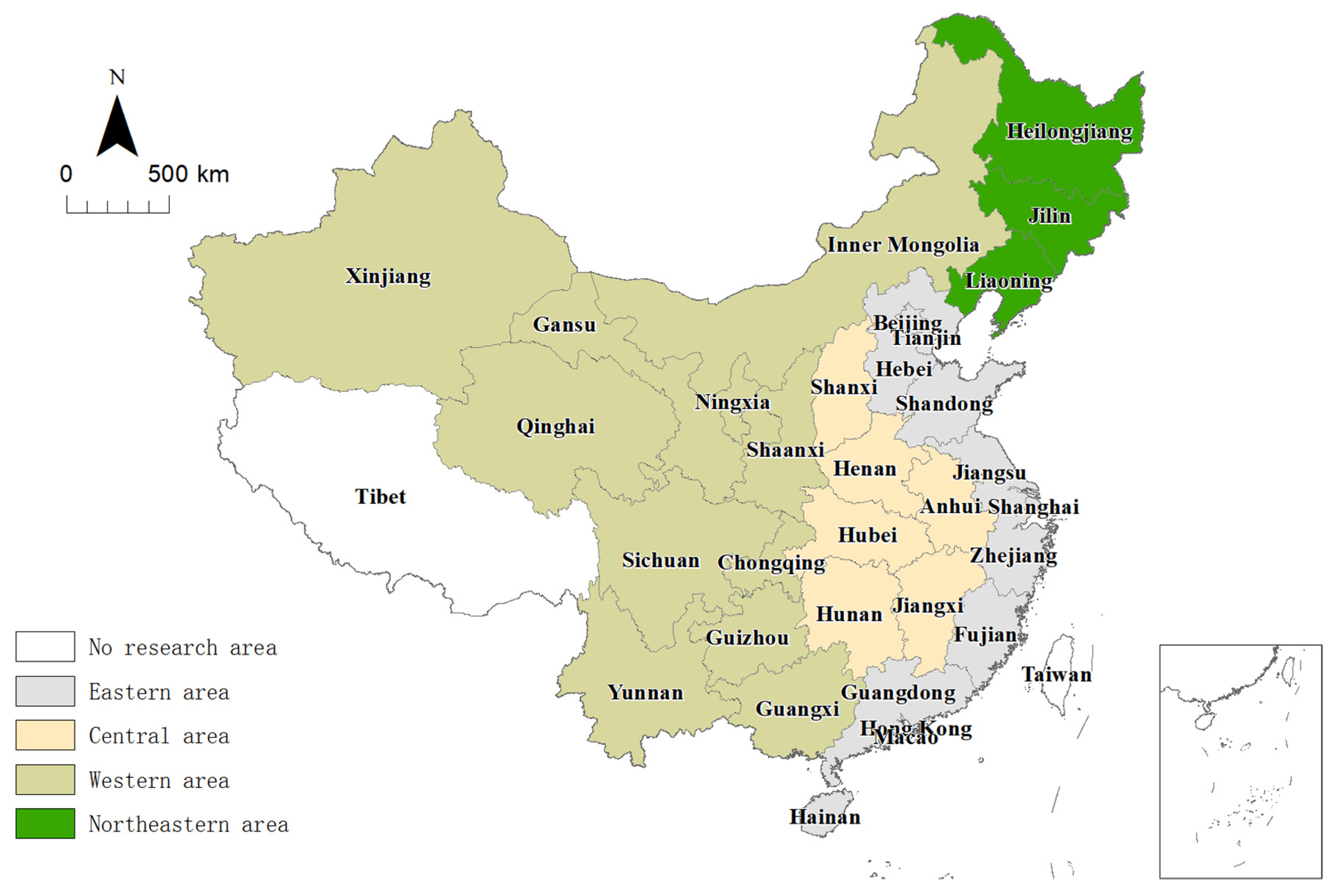
2.1. Research Area
2.1.1. Dependent Variables
2.1.2. Theoretical Mechanism
The Mechanism of Technological Progress
The Mechanism of Government Intervention
The Mechanism of Opening-Up
The Mechanism of Urban Population Density
2.2. Methods
2.2.1. Spatial Autocorrelation Analysis
2.2.2. Spatial Durbin Model
3. Characteristics’ Analyses
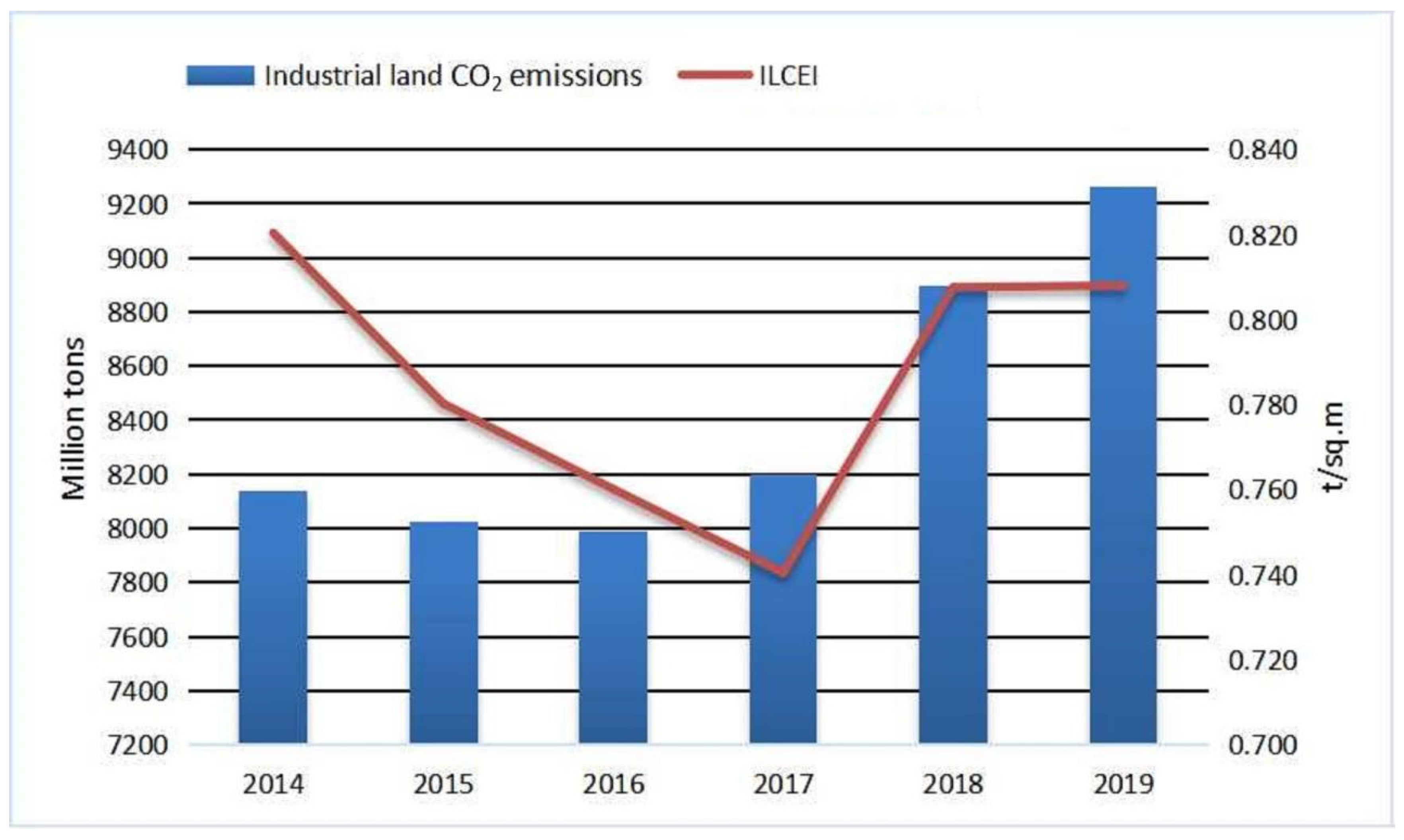
3.1. National Characteristics of ILCEI
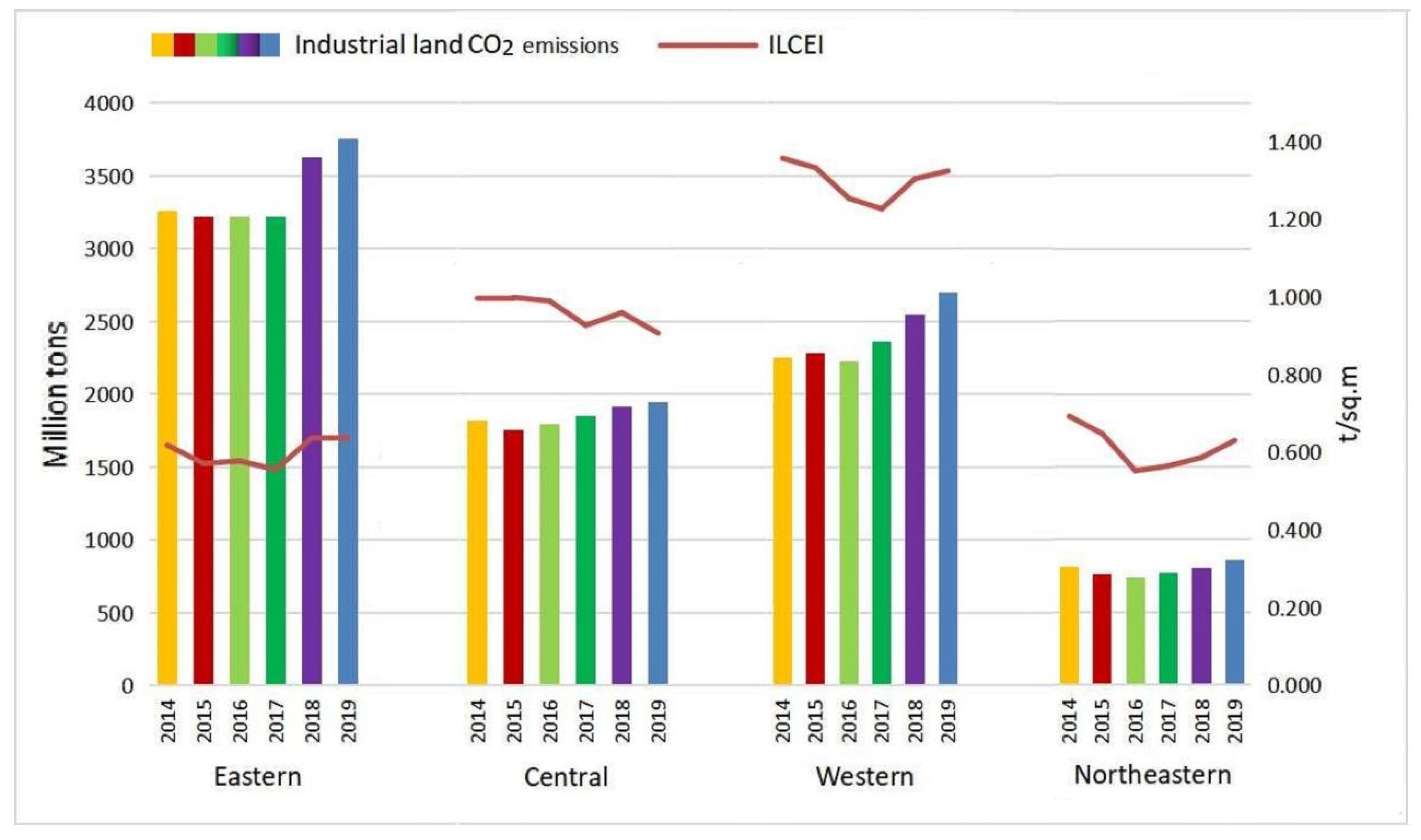
3.2. Regional Characteristics of ILCEI
3.3. Provincial Characteristics of ILCEI
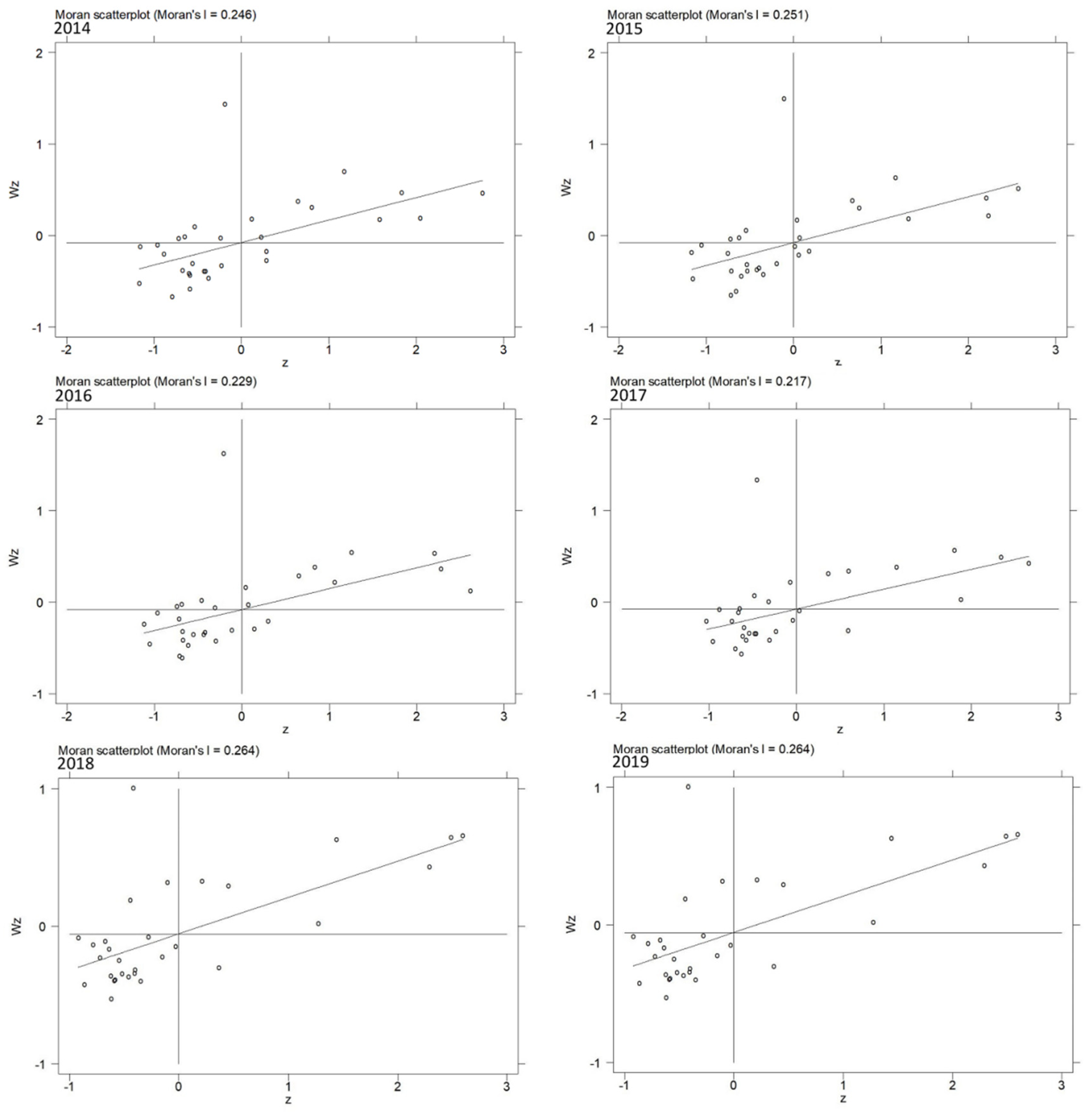
3.4. Spatial Autocorrelation Analysis of ILCEI
4. Regression Analysis
4.1. The Wald and LR Tests
4.2. VIF and Co-Integration Tests
4.3. Discussions of Results
5. Conclusions
Author Contributions
Funding
Institutional Review Board Statement
Informed Consent Statement
Data Availability Statement
Conflicts of Interest
References
- IPCC. Summary for Policymakers/Climate Change 2013: The Physical Science Basis. Contribution of Working Group I to the Fifth Assessment Report of the Intergovernmental Panel on Climate Change; Cambridge University Press: Cambridge, UK, 2013; Available online: https://www.scirp.org/reference/referencespapers.aspx?referenceid=3151617 (accessed on 13 June 2022).
- CO2 Emissions from Fuel Combustion: Highlights; International Energy Agency (IEA). Paris, France. 2019. Available online: https://www.oecd-ilibrary.org/fr/energy/cO2-emissions-from-fuel-combustion-2019_2a701673-en (accessed on 13 June 2022).
- Xi, J.P. Building on Past Achievements and Launching a New Journey for Global Climate Actions. The Belt and Road Reports. Available online: https://www.mfa.gov.cn/ce/cohk/eng/Topics/gjfz/t1839779.htm (accessed on 13 June 2022).
- National Bureau of Statistics of China (NBSC). 2022. Available online: http://data.stats.gov.cn/easyquery.htm?cn=E0103 (accessed on 13 June 2022).
- China Energy Statistical Yearbook (CESY); China Statistical Publishing House: Beijing, China, 2020; Available online: http://tongji.oversea.cnki.net/oversea/engnavi/HomePage.aspx?idN2018070147&nameYCXME&floor¼1 (accessed on 13 June 2022).
- China Urban Construction Statistical Yearboo (CUCSY); Ministry of Housing and Urban-Rural Development: Beijing, China. 2019. Available online: https://data.cnki.net/Yearbook/Single/N2021070166 (accessed on 13 June 2022).
- China Carbon Emission Database (CCED). 2022. Available online: https://www.ceads.net/data/province/energy_inventory/ (accessed on 13 June 2022).
- Liu, N.; Ma, Z.J.; Kang, J.D. Changes in carbon intensity in China’s industrial sector: Decomposition and attribution analysis. Energy Policy 2015, 87, 28–38. [Google Scholar] [CrossRef]
- Wang, Y.; Zheng, Y. Spatial effects of carbon emission intensity and regional development in China. Environ. Sci. Pollut. Res. 2021, 28, 14131–14143. [Google Scholar] [CrossRef] [PubMed]
- Yu, S.W.; Hu, X.; Fan, J.L.; Cheng, J.H. Convergence of carbon emissions intensity across Chinese industrial sectors. J. Clean Prod. 2018, 194, 179–192. [Google Scholar] [CrossRef]
- Luan, B.J.; Huang, J.B.; Cai, X.C.; Zou, H.; Domestic, R.D. technology acquisition, technology assimilation and China’s industrial carbon intensity: Evidence from a dynamic panel threshold model. Sci. Total Environ. 2019, 693, 133436. [Google Scholar] [CrossRef] [PubMed]
- Wang, Y.; Yang, H.X.; Sun, R.X. Effectiveness of China’s provincial industrial carbon emission reduction and optimization of carbon emission reduction paths in “lagging regions”: Efficiency-cost analysis. J. Environ. Manag. 2020, 275, 111221. [Google Scholar] [CrossRef] [PubMed]
- Zhang, X.; Deng, R.R.; Wu, Y.F. Does the green credit policy reduce the carbon emission intensity of heavily polluting industries? -Evidence from China’s industrial sectors. J. Environ. Manag. 2022, 311, 114815. [Google Scholar] [CrossRef]
- Ye, C.S.; Ye, Q.; Shi, X.P.; Sun, Y.P. Technology gap, global value chain and carbon intensity: Evidence from global manufacturing industries. Energy Policy 2020, 137, 111094. [Google Scholar] [CrossRef]
- China Urban Construction Statistical Yearbook (CUCSY), 2015–2019; Ministry of Housing and Urban-Rural Development: Beijing, China. Available online: https://www.mohurd.gov.cn/gongkai/fdzdgknr/sjfb/tjxx/jstjnj/index.html (accessed on 13 June 2022).
- The China Statistical Yearbooks (CSY); China Statistical Publishing House: Beijing, China, 2015–2020. Available online: http://tongji.oversea.cnki.net/oversea/engnavi/HomePage.aspx?id=N2017100312&name=YINFN&floor=1 (accessed on 13 June 2022).
- Lin, P.Q.; Xu, B.; Investment, R.D. Carbon Intensity and Regional Carbon Dioxide Emissions. J. Xiamen Univ. 2020, 4, 70–84. Available online: https://en.cnki.com.cn/Article_en/CJFDTotal-XMDS202004007.htm (accessed on 13 June 2022).
- Shao, W.; Wu, T.L. Intelligence, Factor Market and High-quality Development of Industrial Economy. Inq. Into Econ. Issues 2022, 2, 112–127. Available online: https://kns.cnki.net/kcms/detail/detail.aspx?dbcode=CJFD&dbname=CJFDLAST2022&filename=JJWS202202011&v=MDQwMzNZOUVaWVI4ZVgxTHV4WVM3RGgxVDNxVHJXTTFGckNVUjdpZlllWnVGQ2poVzcvTkx5ZmNmYkc0SE5QTXI= (accessed on 13 June 2022).
- Zeng, L.; Lu, H.; Liu, Y.; Zhou, Y.; Hu, H. Analysis of Regional Differences and Influencing Factors on China’s Carbon Emission Efficiency in 2005–2015. Energies 2019, 12, 3081. [Google Scholar] [CrossRef] [Green Version]
- Chen, F.; Zhao, T.; Liao, Z. The impact of technology-environmental innovation on CO2 emissions in China’s transportation sector. Environ. Sci. Pollut. Res. 2020, 27, 29485–29501. [Google Scholar] [CrossRef]
- Du, Q.; Li, J.; Li, Y.; Huang, N.; Zhou, J.; Li, Z. Carbon inequality in the transportation industry: Empirical evidence from China. Environ. Sci. Pollut. Res. 2020, 27, 6300–6311. [Google Scholar] [CrossRef]
- Lu, H.; Zhao, P.; Hu, H.; Zeng, L.; Wu, K.S.; Lv, D. Transport infrastructure and urban-rural income disparity: A municipal-level analysis in China. J. Transport. Geogr. 2022, 99, 103292. [Google Scholar] [CrossRef]
- Zeng, L.; Li, H.; Wang, X.; Yu, Z.; Hu, H.; Yuan, X.; Zhao, X.; Li, C.; Yuan, D.; Gao, Y.; et al. China’s Transport Land: Spatiotemporal Expansion Characteristics and Driving Mechanism. Land 2022, 11, 1147. [Google Scholar] [CrossRef]
- Tobler, W.R. A computer movie simulating urban growth in the Detroit region. Econ. Geogr. 1970, 46, 234–240. [Google Scholar] [CrossRef]
- Elhorst, J.P. Applied Spatial Econometrics: Raising the Bar. Spat. Econ. Anal. 2010, 5, 9–28. Available online: https://ideas.repec.org/a/taf/specan/v5y2010i1p9-28.html (accessed on 13 June 2022). [CrossRef]
- Chen, Y.; Zhu, B.; Sun, X.; Xu, G. Industrial environmental efficiency and its influencing factors in China: Analysis based on the Super-SBM model and spatial panel data. Environ. Sci. Pollut. Res. 2020, 27, 44267–44278. [Google Scholar] [CrossRef]
- Zhao, L.; Sun, C.; Liu, F. Interprovincial two-stage water resource utilization efficiency under environmental constraint and spatial spillover effects in China. J. Clean. Prod. 2017, 164, 715–725. [Google Scholar] [CrossRef]
- Zhao, P.; Zeng, L.; Li, P.; Lu, H.; Hu, H.; Li, C.; Zheng, M.; Li, H.; Yu, Z.; Yuan, D.; et al. China’s transportation sector carbon dioxide emissions efficiency and its influencing factors based on the EBM DEA model with undesirable outputs and spatial Durbin model. Energy 2022, 238, 121934. [Google Scholar] [CrossRef]
- Li, C.; Shi, H.; Zeng, L.; Dong, X. How Strategic Interaction of Innovation Policies between China’s Regional Governments Affects Wind Energy Innovation. Sustainability 2022, 14, 2543. [Google Scholar] [CrossRef]
- Zhao, P.J.; Zeng, L.E.; Lu, H.Y.; Zhou, Y.; Hu, H.Y.; Wei, X.Y. Green economic efficiency and its influencing factors in China from 2008 to 2017: Based on the super-SBM model with undesirable outputs and spatial Dubin model. Sci. Total Environ. 2020, 741, 140026. [Google Scholar] [CrossRef]
- Zeng, L. China’s Eco-Efficiency: Regional Differences and Influencing Factors Based on a Spatial Panel Data Approach. Sustainability 2021, 13, 3143. [Google Scholar] [CrossRef]
- Ning, L.; Zheng, W.; Zeng, L. Research on China’s Carbon Dioxide Emissions Efficiency from 2007 to 2016: Based on Two Stage Super Efficiency SBM Model and Tobit Model. Beijing Daxue Xuebao (Ziran Kexue Ban)/Acta Sci. Nat. Univ. Pekin 2021, 57, 181–188. Available online: https://www.scopus.com/inward/record.uri?eid=2-s2.0-85101373648&doi=10.13209%2fj.0479-8023.2020.111&partnerID=40&md5=d948ef3627771ac2ca544cbf07fbc229 (accessed on 13 June 2022).
- Li, W.; Huang, Y.; Lu, C. Exploring the driving force and mitigation contribution rate diversity considering new normal pattern as divisions for carbon emissions in Hebei province. J. Clean. Prod. 2020, 243, 118559. [Google Scholar] [CrossRef]
- Gong, P.P.; Song, Z.Y.; Liu, W.D. A Study on Trade Pattern of China with Russia and Central Asia. Geogr. Res. 2015, 34, 812–824. Available online: http://www.dlyj.ac.cn/EN/Y2015/V34/I5/812 (accessed on 13 June 2022).
- Yu, H. Developing China’s Hainan into an International Tourism Destination: How Far Can This Go? East. Asia 2011, 28, 85–113. [Google Scholar] [CrossRef]
- Dong, F.; Zhu, J.; Li, Y.; Chen, Y.; Gao, Y.; Hu, M.; Qin, C.; Sun, J. How green technology innovation affects carbon emission efficiency: Evidence from developed countries proposing carbon neutrality targets. Environ. Sci. Pollut. Res. 2022, 29, 35780–35799. [Google Scholar] [CrossRef] [PubMed]
- Zhang, F.B. Carrying forward the Past and Inheriting Innovation, Comprehensively Improving the Quality of Chemical Higher Education. High. Educ. Chem. Eng. 2019, 36, 6–10, 53. Available online: https://xueshu.baidu.com/usercenter/paper/show?paperid=107e0m60542a0td0g37n0c40g1354845&site=xueshu_se (accessed on 13 June 2022).
- Jiang, F.; Kim, K.A.; Nofsinger, J.R.; Zhu, B. Product market competition and corporate investment: Evidence from China. J. Corp. Financ. 2015, 35, 196–210. [Google Scholar] [CrossRef]
- Jiang, J. Technology Market Development: Comparative Analysis between China and Other Countries. Sci. Technol. Rev. 2020, 38, 25–33. Available online: http://www.kjdb.org/CN/Y2020/V38/I24/25 (accessed on 13 June 2022).


| Regions | Industrial CO2 Emissions (Million Tons) | Industrial Land Area (Square Kilometers) | ||||||||||
|---|---|---|---|---|---|---|---|---|---|---|---|---|
| 2014 | 2015 | 2016 | 2017 | 2018 | 2019 | 2014 | 2015 | 2016 | 2017 | 2018 | 2019 | |
| Beijing | 40.0 | 38.8 | 36.8 | 31.8 | 36.5 | 35.3 | 240.0 | 263.6 | 263.3 | 263.1 | 263.1 | 263.1 |
| Tianjing | 129.8 | 125.1 | 117.7 | 112.0 | 125.9 | 129.9 | 185.9 | 208.9 | 231.2 | 242.5 | 222.4 | 237.7 |
| Hebei | 681.8 | 655.7 | 664.7 | 647.9 | 842.1 | 870.4 | 249.8 | 279.5 | 314.3 | 274.0 | 262.7 | 257.6 |
| Shanghai | 118.3 | 117.1 | 111.2 | 109.1 | 115.2 | 115.4 | 733.1 | 733.1 | 555.8 | 550.6 | 547.5 | 537.7 |
| Jiangsu | 639.8 | 692.2 | 656.2 | 666.4 | 689.7 | 723.9 | 923.6 | 973.8 | 1009.4 | 1064.8 | 1054.8 | 964.5 |
| Zhejiang | 310.1 | 306.2 | 302.3 | 312.2 | 321.4 | 317.0 | 610.7 | 562.3 | 565.7 | 588.5 | 608.8 | 678.5 |
| Fujian | 213.3 | 199.7 | 180.6 | 194.3 | 224.2 | 238.8 | 246.9 | 247.5 | 237.2 | 276.0 | 277.7 | 289.2 |
| Shandong | 699.1 | 730.0 | 737.0 | 705.1 | 807.2 | 842.5 | 934.6 | 1044.1 | 997.1 | 1025.0 | 1069.3 | 1113.4 |
| Guangdong | 395.4 | 325.1 | 385.8 | 408.7 | 431.7 | 451.6 | 1121.5 | 1298.3 | 1375.8 | 1488.0 | 1364.4 | 1554.6 |
| Hainan | 30.5 | 31.6 | 28.6 | 30.5 | 31.4 | 30.9 | 20.1 | 25.6 | 22.3 | 17.0 | 17.4 | 17.8 |
| Eastern | 3258.1 | 3221.5 | 3220.9 | 3218.0 | 3625.2 | 3755.7 | 5266.2 | 5636.7 | 5572.1 | 5789.4 | 5688.1 | 5914.0 |
| Shanxi | 426.7 | 390.9 | 400.0 | 436.9 | 497.6 | 523.5 | 181.7 | 176.6 | 174.7 | 143.3 | 105.8 | 168.6 |
| Anhui | 306.9 | 305.1 | 315.0 | 319.7 | 348.0 | 356.8 | 341.6 | 349.0 | 357.0 | 370.7 | 396.7 | 437.5 |
| Jiangxi | 177.0 | 182.4 | 185.4 | 193.3 | 200.8 | 205.1 | 207.5 | 220.5 | 240.1 | 277.5 | 272.5 | 286.6 |
| Henan | 472.9 | 450.8 | 450.7 | 428.6 | 412.7 | 381.5 | 347.8 | 370.7 | 378.4 | 386.4 | 344.7 | 352.8 |
| Hubei | 232.2 | 227.9 | 230.9 | 242.8 | 242.7 | 262.4 | 549.9 | 443.6 | 460.4 | 573.8 | 611.5 | 624.6 |
| Hunan | 200.1 | 200.3 | 212.1 | 225.1 | 215.9 | 218.1 | 192.8 | 198.1 | 202.0 | 239.7 | 267.0 | 276.4 |
| Central | 1815.8 | 1757.3 | 1794.0 | 1846.4 | 1917.7 | 1947.3 | 1821.3 | 1758.4 | 1812.6 | 1991.5 | 1998.2 | 2146.5 |
| Inner Mongolia | 505.7 | 514.9 | 532.4 | 581.2 | 674.5 | 744.8 | 170.6 | 164.4 | 165.3 | 161.4 | 147.7 | 147.3 |
| Guangxi | 179.4 | 238.9 | 178.9 | 188.9 | 202.1 | 218.8 | 174.6 | 199.8 | 204.1 | 220.5 | 208.5 | 206.5 |
| Chongqing | 126.8 | 128.2 | 119.1 | 121.1 | 127.3 | 120.3 | 218.6 | 236.0 | 246.8 | 244.6 | 252.6 | 262.6 |
| Sichuan | 276.7 | 257.1 | 234.9 | 231.6 | 218.9 | 235.5 | 428.1 | 410.6 | 441.8 | 450.8 | 480.1 | 482.4 |
| Guizhou | 166.9 | 163.5 | 175.2 | 177.3 | 182.7 | 191.8 | 109.7 | 122.2 | 122.9 | 155.2 | 161.0 | 162.3 |
| Yunnan | 152.7 | 132.5 | 135.4 | 149.3 | 164.0 | 135.5 | 104.4 | 106.7 | 111.2 | 122.6 | 126.6 | 126.7 |
| Shaanxi | 237.0 | 239.0 | 230.9 | 227.8 | 240.1 | 260.1 | 118.2 | 129.5 | 132.4 | 146.0 | 149.6 | 174.6 |
| Gansu | 139.6 | 132.9 | 124.8 | 122.8 | 137.1 | 138.3 | 129.8 | 122.6 | 129.7 | 171.4 | 173.3 | 200.5 |
| Qinghai | 39.3 | 41.5 | 46.4 | 41.3 | 39.6 | 39.2 | 12.4 | 13.1 | 13.2 | 13.2 | 13.3 | 14.5 |
| Ningxia | 135.5 | 133.3 | 129.3 | 167.4 | 185.2 | 205.5 | 35.4 | 38.6 | 41.1 | 42.6 | 43.0 | 45.4 |
| Xinjiang | 293.3 | 302.7 | 321.7 | 352.7 | 373.1 | 410.3 | 158.0 | 170.5 | 168.5 | 196.1 | 194.6 | 215.5 |
| Western | 2253.1 | 2284.6 | 2229.0 | 2361.4 | 2544.5 | 2700.2 | 1659.8 | 1713.9 | 1777.0 | 1924.3 | 1950.3 | 2038.3 |
| Liaoning | 416.2 | 399.1 | 383.2 | 404.3 | 446.6 | 459.7 | 570.5 | 565.0 | 711.7 | 719.3 | 719.2 | 707.1 |
| Jilin | 188.5 | 169.9 | 163.9 | 169.2 | 170.0 | 177.7 | 269.0 | 260.6 | 274.7 | 286.8 | 296.0 | 300.4 |
| Heilongjiang | 208.0 | 192.7 | 194.7 | 196.7 | 189.9 | 222.7 | 334.3 | 350.6 | 357.5 | 357.7 | 360.4 | 357.9 |
| Northeastern | 812.7 | 761.7 | 741.8 | 770.1 | 806.4 | 860.1 | 1173.7 | 1176.2 | 1344.0 | 1363.8 | 1375.6 | 1365.5 |
| China | 8139.7 | 8025.2 | 7985.7 | 8195.9 | 8893.8 | 9263.4 | 9921.1 | 10,285 | 10,506 | 11,069 | 11,012 | 11,464 |
| Explanatory Variable | Variables’ Definitions and Units | Pre-Judgment |
|---|---|---|
| R & D personnel (RDP) | R & D personnel of industrial enterprises above designated size (person) | Negative |
| Technology market (TM) | The proportion of the total value of technical market to GDP (%) | Negative |
| Governmental intervention (GI) | The proportion of the financial expenditure to GDP (%) | Unknown |
| Foreign trade dependence (FTD) | The proportion of the foreign trade to GDP (%) | Unknown |
| Foreign direct investment (FDI) | The proportion of the foreign direct Investment to GDP (%) | Unknown |
| Urban population density (UPD) | Population density of urban area (person/sq.km) | Unknown |
| Regions | 2014 | 2015 | 2016 | 2017 | 2018 | 2019 | Mean |
|---|---|---|---|---|---|---|---|
| Beijing | 0.167 | 0.147 | 0.14 | 0.121 | 0.139 | 0.134 | 0.141 |
| Tianjing | 0.698 | 0.599 | 0.509 | 0.462 | 0.566 | 0.546 | 0.563 |
| Hebei | 2.729 | 2.346 | 2.115 | 2.365 | 3.206 | 3.38 | 2.690 |
| Shanghai | 0.161 | 0.160 | 0.200 | 0.198 | 0.210 | 0.215 | 0.191 |
| Jiangsu | 0.693 | 0.711 | 0.65 | 0.626 | 0.654 | 0.751 | 0.681 |
| Zhejiang | 0.508 | 0.545 | 0.534 | 0.531 | 0.528 | 0.467 | 0.519 |
| Fujian | 0.864 | 0.807 | 0.761 | 0.704 | 0.807 | 0.826 | 0.795 |
| Shandong | 0.748 | 0.699 | 0.739 | 0.688 | 0.755 | 0.757 | 0.731 |
| Guangdong | 0.353 | 0.250 | 0.280 | 0.275 | 0.316 | 0.291 | 0.294 |
| Hainan | 1.518 | 1.232 | 1.283 | 1.797 | 1.808 | 1.742 | 1.563 |
| Eastern | 0.619 | 0.572 | 0.578 | 0.556 | 0.637 | 0.635 | 0.600 |
| Shanxi | 2.348 | 2.213 | 2.290 | 3.048 | 4.701 | 3.105 | 2.951 |
| Anhui | 0.898 | 0.874 | 0.882 | 0.862 | 0.877 | 0.816 | 0.868 |
| Jiangxi | 0.853 | 0.827 | 0.772 | 0.696 | 0.737 | 0.716 | 0.767 |
| Henan | 1.360 | 1.216 | 1.191 | 1.109 | 1.197 | 1.081 | 1.192 |
| Hubei | 0.422 | 0.514 | 0.501 | 0.423 | 0.397 | 0.420 | 0.446 |
| Hunan | 1.038 | 1.011 | 1.05 | 0.939 | 0.809 | 0.789 | 0.939 |
| Central | 0.997 | 0.999 | 0.99 | 0.927 | 0.96 | 0.907 | 0.963 |
| Inner Mongolia | 2.964 | 3.133 | 3.22 | 3.601 | 4.565 | 5.055 | 3.756 |
| Guangxi | 1.027 | 1.195 | 0.877 | 0.857 | 0.969 | 1.060 | 0.998 |
| Chongqing | 0.580 | 0.543 | 0.483 | 0.495 | 0.504 | 0.458 | 0.511 |
| Sichuan | 0.646 | 0.626 | 0.532 | 0.514 | 0.456 | 0.488 | 0.544 |
| Guizhou | 1.521 | 1.338 | 1.426 | 1.142 | 1.134 | 1.182 | 1.291 |
| Yunnan | 1.463 | 1.242 | 1.218 | 1.218 | 1.295 | 1.069 | 1.251 |
| Shaanxi | 2.006 | 1.846 | 1.744 | 1.561 | 1.605 | 1.490 | 1.709 |
| Gansu | 1.075 | 1.084 | 0.962 | 0.717 | 0.791 | 0.690 | 0.887 |
| Qinghai | 3.163 | 3.157 | 3.522 | 3.125 | 2.991 | 2.703 | 3.110 |
| Ningxia | 3.827 | 3.457 | 3.149 | 3.93 | 4.306 | 4.524 | 3.866 |
| Xinjiang | 1.857 | 1.776 | 1.91 | 1.799 | 1.917 | 1.905 | 1.861 |
| Western | 1.357 | 1.333 | 1.254 | 1.227 | 1.305 | 1.325 | 1.300 |
| Liaoning | 0.730 | 0.706 | 0.538 | 0.562 | 0.621 | 0.650 | 0.635 |
| Jilin | 0.701 | 0.652 | 0.597 | 0.590 | 0.574 | 0.592 | 0.618 |
| Heilongjiang | 0.622 | 0.550 | 0.545 | 0.55 | 0.527 | 0.622 | 0.569 |
| Northeastern | 0.692 | 0.648 | 0.552 | 0.565 | 0.586 | 0.630 | 0.612 |
| China | 0.619 | 0.572 | 0.578 | 0.556 | 0.637 | 0.635 | 0.600 |
| Regions | 2014 | 2015 | 2016 | 2017 | 2018 | 2019 | Mean |
|---|---|---|---|---|---|---|---|
| Eastern | 0.619 | 0.572 | 0.578 | 0.556 | 0.637 | 0.635 | 0.600 |
| Central | 0.997 | 0.999 | 0.99 | 0.927 | 0.960 | 0.907 | 0.963 |
| Western | 1.357 | 1.333 | 1.254 | 1.227 | 1.305 | 1.325 | 1.300 |
| Northeastern | 0.692 | 0.648 | 0.552 | 0.565 | 0.586 | 0.630 | 0.612 |
| China | 0.619 | 0.572 | 0.578 | 0.556 | 0.637 | 0.635 | 0.600 |
| Year | Global Moran’s I | Z-Score | p-Value |
|---|---|---|---|
| 2014 | 0.246 *** | 2.999 | 0.003 |
| 2015 | 0.251 *** | 3.056 | 0.002 |
| 2016 | 0.229 *** | 2.821 | 0.005 |
| 2017 | 0.217 *** | 2.704 | 0.007 |
| 2018 | 0.264 *** | 3.235 | 0.001 |
| 2019 | 0.222 *** | 2.837 | 0.005 |
| Fixed Effects | Random Effects | |
|---|---|---|
| Wald test spatial lag | 45.52 *** | 36.00 *** |
| LR test spatial lag | 42.29 *** | 33.29 *** |
| Wald test spatial error | 44.58 *** | 31.38 *** |
| LR test spatial error | 62.06 *** | 29.38 *** |
| RDP | TM | GI | FTD | FDI | UPD | Mean VIF | |
|---|---|---|---|---|---|---|---|
| VIF | 7.32 | 1.29 | 7.51 | 1.62 | 1.65 | 1.11 | 3.42 |
| 1/VIF | 0.137 | 0.775 | 0.133 | 0.617 | 0.606 | 0.901 |
| LLC | Fisher-ADF | PP-ADF | |
|---|---|---|---|
| InILCEI | −4.71747 *** | 55.1809 | 67.7630 |
| InRDP | −9.39487 *** | 76.7227 * | 113.816 *** |
| InTM | −5.82977 *** | 90.5035 *** | 126.535 *** |
| InGI | −0.96485 | 38.2175 | 33.9923 |
| InFTD | 3.04179 *** | 27.0252 | 26.5892 |
| InFDI | −14.7583 *** | 49.1062 | 52.2592 |
| InUPD | −13.4544 *** | 79.2340 ** | 98.7717 *** |
| ΔInILCEI | −17.5301 *** | 99.2307 *** | 113.333 *** |
| ΔInRDP | −15.4006 *** | 92.2719 *** | 106.558 *** |
| ΔInTM | −17.8624 *** | −6.97951 *** | 129.987 *** |
| ΔInGI | −5.95718 *** | 62.6942 | 65.4803 |
| ΔInFTD | −17.3686 *** | 65.2239 | 68.0295 |
| ΔInFDI | −25.8630 *** | 120.086 *** | 140.144 *** |
| ΔInUPD | −54.8441 *** | 109.315 *** | 130.428 *** |
| ΔΔInILCEI | −25.2679 *** | 146.034 *** | 163.233 *** |
| ΔΔInRDP | −55.7402 *** | 145.721 *** | 165.895 *** |
| ΔΔInTM | −736.844 *** | 142.570 *** | 165.242 *** |
| ΔΔInGI | −8.63430 *** | 79.0983 ** | 90.9410 *** |
| ΔΔInFTD | −133.564 *** | −133.564 *** | 123.301 *** |
| ΔΔInFDI | −38.0943 *** | 171.338 *** | 192.268 *** |
| ΔΔInUPD | −41.3728 *** | 188.040 *** | 207.668 *** |
| Spatial Fixed Effects | Time Fixed Effects | Spatial and Time Fixed Effects | |
|---|---|---|---|
| InRDP | −0.111 ** | −0.093 | −0.097 ** |
| InTM | −0.002 | −0.223 *** | −0.007 |
| InGI | 0.187 | −0.465 * | 0.163 |
| InFTD | −0.067 | −0.559 *** | −0.081 *** |
| InFDI | −0.002 | −0.065 | −0.026 |
| InUPD | 0.201 *** | −0.081 | 0.248 *** |
| W*InRDP | −0.061 | 0.146 | −0.079 |
| W*InTM | 0.076 ** | 0.315 *** | 0.159 *** |
| W*InGI | 0.536 ** | 0.224 | 0.994 ** |
| W*InFTD | 0.549 *** | 0.274 | 0.381 ** |
| W*InFDI | 0.0227 | −0.246 ** | −0.003 |
| W*InUPD | 0.620 *** | −0.861 *** | 0.880 *** |
| Spatial rho | 0.327 *** | 0.366 *** | 0.341 ** |
| Variance sigma2_e | 0.009 *** | 0.145 *** | 0.008 *** |
| R-squared | 0.175 | 0.730 | 0.198 |
| Log-likelihood | 171.077 | −84.369 | 177.517 |
Publisher’s Note: MDPI stays neutral with regard to jurisdictional claims in published maps and institutional affiliations. |
© 2022 by the authors. Licensee MDPI, Basel, Switzerland. This article is an open access article distributed under the terms and conditions of the Creative Commons Attribution (CC BY) license (https://creativecommons.org/licenses/by/4.0/).
Share and Cite
Zeng, L.; Li, C.; Liang, Z.; Zhao, X.; Hu, H.; Wang, X.; Yuan, D.; Yu, Z.; Yang, T.; Lu, J.; et al. The Carbon Emission Intensity of Industrial Land in China: Spatiotemporal Characteristics and Driving Factors. Land 2022, 11, 1156. https://doi.org/10.3390/land11081156
Zeng L, Li C, Liang Z, Zhao X, Hu H, Wang X, Yuan D, Yu Z, Yang T, Lu J, et al. The Carbon Emission Intensity of Industrial Land in China: Spatiotemporal Characteristics and Driving Factors. Land. 2022; 11(8):1156. https://doi.org/10.3390/land11081156
Chicago/Turabian StyleZeng, Liangen, Chengming Li, Zhongqi Liang, Xuhai Zhao, Haoyu Hu, Xiao Wang, Dandan Yuan, Zhao Yu, Tingzhang Yang, Jingming Lu, and et al. 2022. "The Carbon Emission Intensity of Industrial Land in China: Spatiotemporal Characteristics and Driving Factors" Land 11, no. 8: 1156. https://doi.org/10.3390/land11081156