
Simulating the Spatial Mismatch between Ecosystem Services’ (ESs’) Supply and Demand Based on Their Spatial Transfer in Urban Agglomeration Area, China


Abstract
:1. Introduction
2. Methods
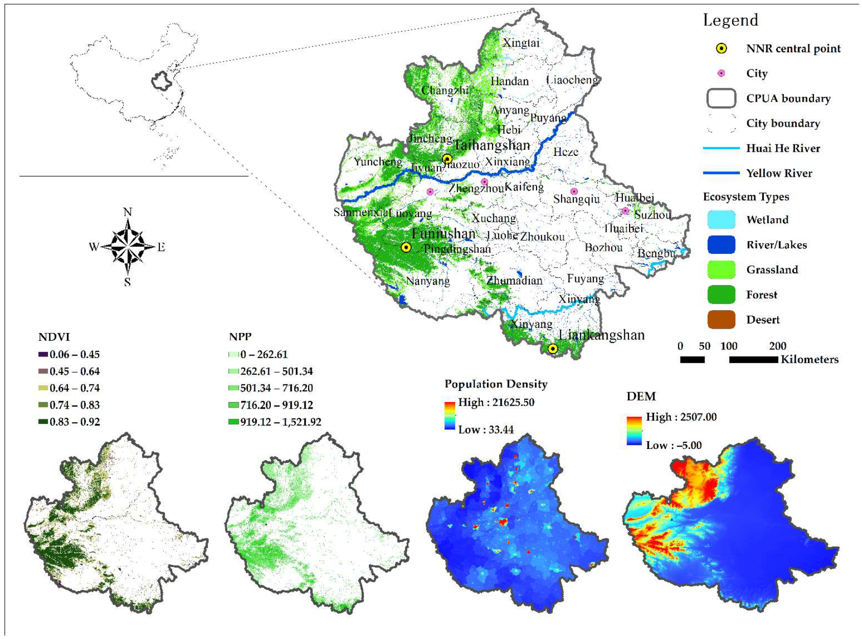
2.1. Study Area
2.2. Data and Pretreatment
2.3. ES Calculation Method and Process
2.4. ES Spatial Transfer (the Breaking Point Model)
2.5. Spatial Boundary Condition Determination
3. Results
3.1. ES amount and Distribution
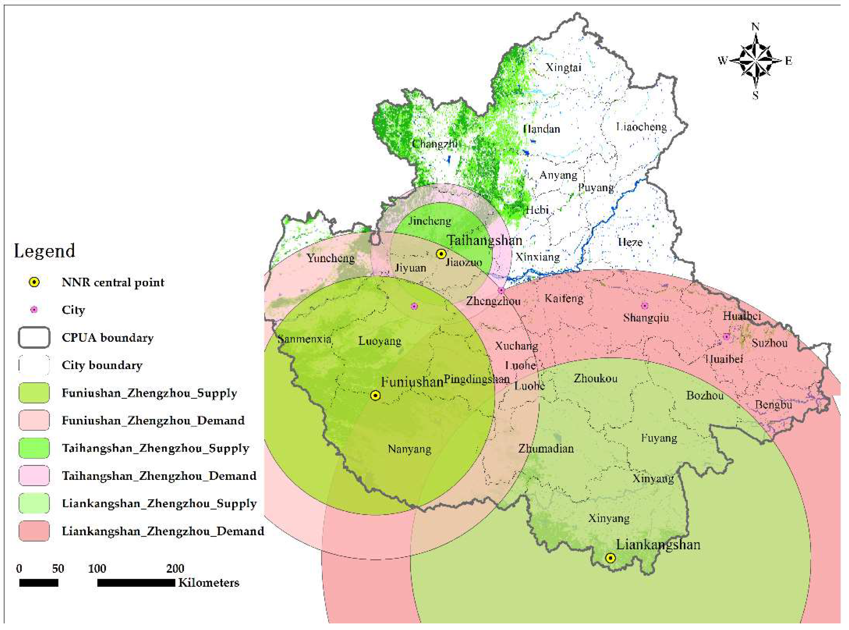
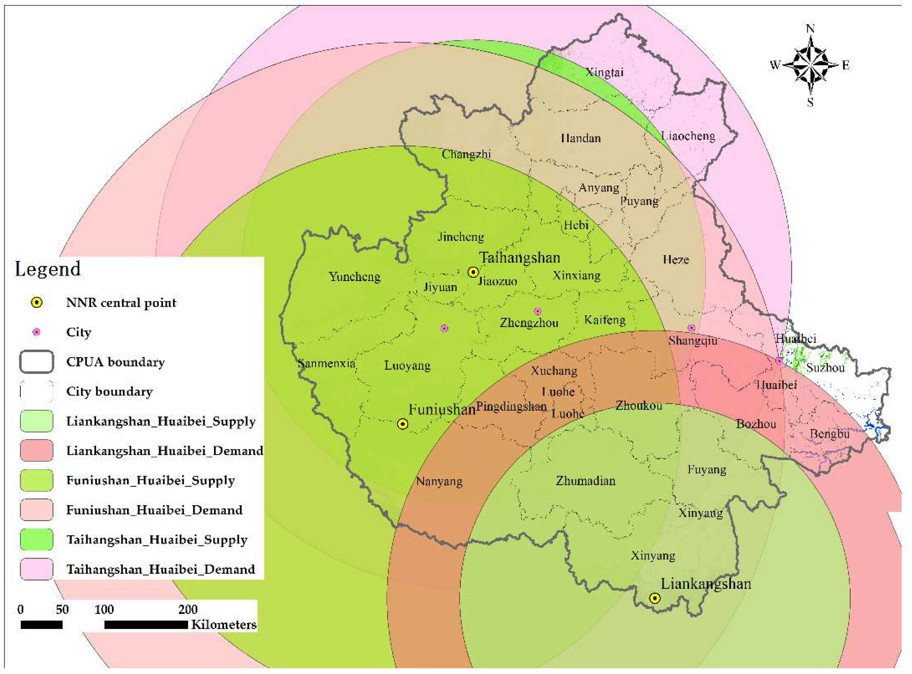
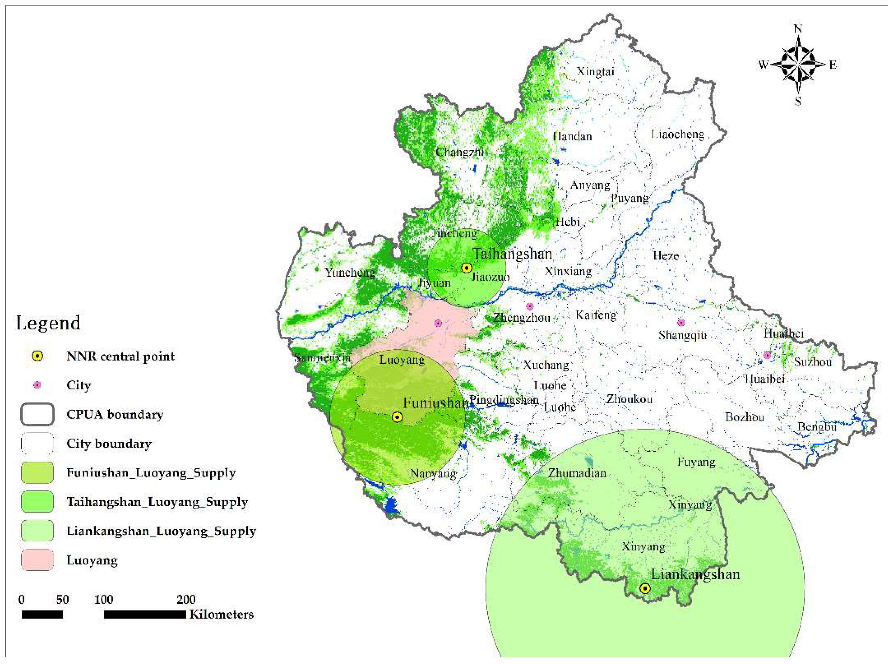
3.2. ES in the Transfer-Out Area and Transfer Radiation Scope
3.3. ES Spatial Transfer Radius
3.4. ES supply and Demand Patterns Based on Its Spatial Transfer
4. Discussion
4.1. Implications
4.2. Limitations
5. Conclusions
Author Contributions
Funding
Institutional Review Board Statement
Informed Consent Statement
Data Availability Statement
Acknowledgments
Conflicts of Interest
References
- Costanza, R.; D’Arge, R.; Groot, R.D.; Farber, S.; Grasso, M.; Hannon, B.; Limburg, K.; Naeem, S.; O’Neill, R.V.; Paruelo, J. The value of the world’s ecosystem services and natural capital. Nature 1997, 387, 253–260. [Google Scholar] [CrossRef]
- Daily, G.C. (Ed.) Nature’s Services: Societal Dependence on Natural Ecosystems; Island Press: Washington, DC, USA, 1997. [Google Scholar]
- Breslow, S.J.; Allen, M.; Holstein, D.; Sojka, B.; Barnea, R.; Basurto, X.; Carothers, C.; Charnley, S.; Coulthard, S.; Dolšak, N.; et al. Evaluating indicators of human well-being for ecosystem-based management. Ecosyst. Health Sustain. 2017, 3, 1–18. [Google Scholar] [CrossRef]
- Burkhard, B.; Kandziora, M.; Hou, Y.; Müller, F. Ecosystem service potentials, flows and demands-concepts for spatial localisation, indication and quantification. Landsc. Online 2014, 34, 1–32. [Google Scholar] [CrossRef]
- Xie, G.; Lu, C.; Leng, Y.; Zheng, D.; Li, S. Ecological assets valuation of the Tibetan Plateau. J. Nat. Resour. 2003, 18, 189–197. [Google Scholar] [CrossRef]
- Xie, G.; Zhen, L.; Lu, C.; Xiao, Y.; Chen, C. Expert Knowledge Based Valuation Method of Ecosystem Services in China. J. Nat. Resour. 2008, 23, 911–919. [Google Scholar] [CrossRef]
- Yu, Z.; Fryd, O.; Sun, R.; Jørgensen, G.; Yang, G.; Özdil, N.C.; Vejre, H. Where and how to cool? An idealized urban thermal security pattern model. Landsc. Ecol. 2021, 36, 2165–2174. [Google Scholar] [CrossRef]
- Reid, W.V.; Mooney, H.A.; Cropper, A.; Capistrano, D.; Zurek, M.B. Millennium Ecosystem Assessment Synthesis Report; World Resources Institute: Washington, DC, USA, 2005. [Google Scholar]
- Burkhard, B.; Kroll, F.; Nedkov, S.; Müller, F. Mapping ecosystem service supply, demand and budgets. Ecol. Indic. 2012, 21, 17–29. [Google Scholar] [CrossRef]
- Cai, W.; Wu, T.; Jiang, W.; Peng, W.; Cai, Y. Integrating Ecosystem Services Supply—Demand and Spatial Relationships for Intercity Cooperation: A Case Study of the Yangtze River Delta. Sustainability 2020, 12, 4131. [Google Scholar] [CrossRef]
- Villamagna, A.M.; Angermeier, P.L.; Bennet, E.M. Capacity, pressure, demand, and flow: Aconceptual framework for analyzing ecosystem service provision and delivery. Ecol. Complex. 2013, 15, 114–121. [Google Scholar] [CrossRef]
- Kroll, F.; Müller, F.; Haase, D.; Fohrer, N. Rural-urban gradient analysis of ecosystem services supply and demand dynamics. Land Use Policy 2012, 29, 521–535. [Google Scholar] [CrossRef]
- Chen, J.; Jiang, B.; Bai, Y.; Xu, X.; Alatalo, J.M. Quantifying ecosystem services supply and demand shortfalls and mismatches for management optimisation. Sci. Total Environ. 2019, 650, 1426–1439. [Google Scholar] [CrossRef]
- Jiang, B.; Bai, Y.; Chen, J.; Alatalo, J.M.; Xu, X.; Liu, G.; Wang, Q. Land management to reconcile ecosystem services supply and demand mismatches—A case study in Shanghai municipality, China. Land Degrad. Dev. 2020, 31, 2684–2699. [Google Scholar] [CrossRef]
- Kaminski, A.; Bauer, D.M.; Bell, K.P.; Loftin, C.S.; Nelson, E.J. Using landscape metrics to characterize towns along an urban-rural gradient. Landsc. Ecol. 2021, 36, 2937–2956. [Google Scholar] [CrossRef]
- Zhou, W.; Fisher, B.; Pickett, S.T. Cities are hungry for actionable ecological knowledge. Front. Ecol. Environ. 2019, 17, 135. [Google Scholar] [CrossRef]
- McHale, M.R.; Beck, S.M.; Pickett, S.T.A.; Childers, D.L.; Cadenasso, M.L.; Rivers, L.; Swemmer, L.; Ebersohn, L.; Twine, W.; Bunn, D.N. Democratization of ecosystem services—A radical approach for assessing nature’s benefits in the face of urbanization. Ecosyst. Health Sustain. 2018, 4, 115–131. [Google Scholar] [CrossRef]
- Shen, J.; Wang, Y. Allocating and mapping ecosystem service demands with spatial flow from built-up areas to natural spaces. Sci. Total Environ. 2021, 798, 149330. [Google Scholar] [CrossRef]
- Xiao, Y.; Xie, G.; Lu, C.; Xu, J. Involvement of ecosystem service flows in human wellbeing based on the relationship between supply and demand. Acta Ecol. Sin. 2016, 36, 3096–3103. [Google Scholar] [CrossRef]
- Liu, M.; Fan, J.; Wang, Y.; Hu, C. Study on Ecosystem Service Value (ESV) Spatial Transfer in the Central Plains Urban Agglomeration in the Yellow River Basin, China. Int. J. Environ. Res. Public Health 2021, 18, 9751. [Google Scholar] [CrossRef]
- Qiao, X.; Yang, Y.; Yang, D. Assessment of Ecosystem Service value Transfer in Weigan River Basin, Xinjiang, China. J. Desert Res. 2011, 31, 1008–1014. [Google Scholar]
- Guo, Z.; Li, D. Transfer of Value of Biodiversity and Method of Valuation of Process—Benefit. Sci. Technol. Rev. 1997, 58–60. Available online: https://d.wanfangdata.com.cn/periodical/QK199700782210 (accessed on 30 March 2017).
- Shi, P.; Zhang, S.; Pan, Y.; Wang, J.; Hong, S.; Shen, P.; Zhu, W.; Ye, T. Ecosystem Capital and Regional Sustainable Development. J. Beijing Norm. Univ. (Soc. Sci.) 2005, 2005, 131–137. [Google Scholar]
- Ouyang, X.; He, Q.; Zhu, X. Simulation of Impacts of Urban Agglomeration Land Use Change on Ecosystem Services Value under Multi-Scenarios: Case Study in Changsha-Zhuzhou-Xiangtan Urban agglomeration. Econ. Geogr. 2020, 40, 93–102. [Google Scholar] [CrossRef]
- Zhang, D.; Huang, Q.; He, C.; Yin, D.; Liu, Z. Planning urban landscape to maintain key ecosystem services in a rapidly urbanizing area: A scenario analysis in the Beijing-Tianjin-Hebei urban agglomeration, China. Ecol. Indic. 2019, 96, 559–571. [Google Scholar] [CrossRef]
- Gao, J. New Characteristics and New Requirements for the Development of Central Plains Urban Agglomeration. Available online: http://newpaper.dahe.cn/hnrb/html/2017-03/30/content_133017.htm (accessed on 30 March 2017).
- Luo, Q.; Zhou, J.; Li, Z.; Yu, B. Spatial differences of ecosystem services and their driving factors: A comparation analysis among three urban agglomerations in China’s Yangtze River Economic Belt. Sci. Total Environ. 2020, 725, 138452. [Google Scholar] [CrossRef] [PubMed]
- Yu, Y.; Han, P.; Yang, N.; Li, X.; Guo, J. Research of Carrying Capacity on Resource and environment in Core Cities of Central Henan Urban Agglomeration. Acta Sci. Nat. Univ. Pekin. 2018, 54, 407–414. [Google Scholar] [CrossRef]
- Zheng, H.; Wang, L.; Peng, W.; Zhang, C.; Li, C.; Robinson, B.E.; Wu, X.; Kong, L.; Li, R.; Xiao, Y.; et al. Realizing the values of natural capital for inclusive, sustainable development: Informing China’s new ecological development strategy. Proc. Natl. Acad. Sci. USA 2019, 116, 8623–8628. [Google Scholar] [CrossRef]
- Fang, C.; Song, J.; Zhang, Q.; Li, M. The Formation, Development and Spatial Heterogeneity Patterns for the Structures System of Urban Agglomerations in China. Acta Geogr. Sin. 2005, 60, 827–840. [Google Scholar] [CrossRef]
- Luo, X.; Jiang, P.; Yang, J.; Jin, J.; Yang, J. Simulating PM2.5 removal in an urban ecosystem based on the social-ecological model framework. Ecosyst. Serv. 2021, 47, 101234. [Google Scholar] [CrossRef]
- Ouyang, X.; Zhu, X. Spatio-temporal characteristics of urban land expansion in Chinese urban agglomerations. Acta Geogr. Sin. 2020, 75, 18. [Google Scholar] [CrossRef]
- Pan, Y.; Shi, P.; Zhu, W.; Gu, X.; Fan, Y.; Li, J. Valuation of the Ecological Assets by Terrestrial Ecosystems in China Based on Remote Sensing. Sci. China Ser. D 2004, 34, 375–385. [Google Scholar] [CrossRef]
- Lu, F.; Hu, H.; Sun, W.; Zhu, J.; Liu, G.; Zhou, W.; Zhang, Q.; Shi, P.; Liu, X.; Wu, X.; et al. Effects of national ecological restoration projects on carbon sequestration in China from 2001 to 2010. Proc. Natl. Acad. Sci. USA 2018, 115, 4039–4044. [Google Scholar] [CrossRef]
- Wang, F.; Lv, J. The evaluation and spatial-temporal evolvement of the city competitiveness of Zhongyuan Urban Agglomeration. Geogr. Res. 2011, 30, 49–60. [Google Scholar] [CrossRef]
- National Development and Reform Commission. Development Planning of the Central Plains Urban Agglomeration; National Development and Reform Commission: Beijing, China, 2017; Volume 2017. [Google Scholar]
- Wang, W.; Sun, T.; Wang, J. Annual Dynamic Monitoring of Regional Ecosystem Service Value Based on Multi-source Remote Sensing Data: A Case of Central Plains Urban Agglomeration Region. Sci. Geogr. Sin. 2019, 39, 680–687. [Google Scholar] [CrossRef]
- Chen, J.; Li, T. Changes of Spatial Variations in Ecosystem Service Value in China. Acta Sci. Nat. Univ. Pekin. 2019, 55, 951–961. [Google Scholar] [CrossRef]
- Fan, X.; Gao, J.; Wen, W. Exploratory Study on Eco-Assets Transferring and the VaIuating Models. Res. Environ. Sci. 2007, 20, 160–164. [Google Scholar]
- Yang, C. Study on Spatial-Temporal Differentiation of Land Ecosystem Service Value and Driving Factors in Central Plains Urban Agglomeration. Master’s Thesis, Hebei University of Economics and Business, Shijiazhuang, China, 2018. [Google Scholar]
- Li, X.; Li, G.; Zeng, G.; Qin, C.; Zhang, W. Economic Geography, 3rd ed.; Higher Education Press: Beijing, China, 2019; p. 189. [Google Scholar]
- Youngquist, M.B.; Boone, M.D. Making the connection—Combining habitat suitability and landscape connectivity to understand species distribution in an agricultural landscape. Landsc. Ecol. 2021, 36, 2795–2809. [Google Scholar] [CrossRef]
- Cheng, H.; Li, X.; Khanal, L.; Xuelong, J. Habitat suitability and connectivity inform a co-management policy of protected area network for Asian elephants in China. PeerJ 2019, 7, e6791. [Google Scholar] [CrossRef]
- Karimi, J.D.; Harris, J.A.; Corstanje, R. Using Bayesian Belief Networks to assess the influence of landscape connectivity on ecosystem service trade-offs and synergies in urban landscapes in the UK. Landsc. Ecol. 2021, 36, 3345–3363. [Google Scholar] [CrossRef]
- Jing, W.B.; Jie, S.; Jun, H.X. Comprehensive identification of eco-corridors and eco-nods based on principle of hydrological analysis and linkage mapper. Acta Ecol. Sin. 2022, 42, 2995–3009. [Google Scholar]
- Zhou, W.; Wang, K.; Yu, W.; Li, W.; Han, L.; Qian, Y. Understanding the social and ecological connections between cities and surrounding regions for urban and regional sustainability. Acta Ecol. Sin. 2017, 37, 5238–5245. [Google Scholar]
- Wang, Z.; Liu, L. Ecosystem structure and functioning: Current knowledge and perspectives. Chin. J. Plant Ecol. 2021, 45, 1033–1035. [Google Scholar] [CrossRef]
- Niu, T.; Yue, D.; Zhang, Q.; Yu, Q.; Su, K. Spatial Structure and Characteristics of Potential Ecological Networks. Trans. Chin. Soc. Agric. Mach. 2019, 50, 166–175. [Google Scholar]
- Shu, F.; Zhengyu, T.; Lu, Y.; Chen, G.; Moxi, T. Collaborative construction of ecological network in urban agglomerations: A case of Guangdong-Hongkong-Macao Great Bay area. Acta Ecol. Sin. 2022, 42, 1–16. [Google Scholar] [CrossRef]
- Guo, Z.; Gan, Y. Some scientific questions for ecosystem services. Biodivers. Sci. 2003, 11, 63–70. [Google Scholar] [CrossRef]
- Luo, Y.; Wu, J.; Wang, X.; Zhao, Y.; Feng, Z. Understanding ecological groups under landscape fragmentation based on network theory. Landsc. Urban Plan. 2021, 210, 104066. [Google Scholar] [CrossRef]
- Bureau, L.E.E. Monthly Environmental Monitoring Report. Available online: http://sthj.ly.gov.cn/Article?cateID=78 (accessed on 20 July 2022).
- Bureau, Z.W.C. Zhengzhou Water Resources Bulletin. Available online: http://public.zhengzhou.gov.cn/D12Y/6283515.jhtml (accessed on 20 July 2022).
- Shen, J.; Guo, X.; Wang, Y. Identifying and setting the natural spaces priority based on the multi-ecosystem services capacity index. Ecol. Indic. 2021, 125, 107473. [Google Scholar] [CrossRef]


| Ecosystems | Land Use/Land Cover |
|---|---|
| Forest | mainly includes dense forest land (forest land), shrub land, sparse forest land, and other forest land; |
| Grassland | mainly includes high-coverage grassland, medium-coverage grassland, and low-coverage grassland; |
| Wetland | mainly includes marsh and beach; |
| Rivers/lakes | mainly includes rivers, lakes, reservoirs, glaciers, and permanent snow; |
| Desert | Sandy land, Gobi desert, saline-alkali land; Alpine desert. |
| Ecosystem Services | Forest | Grassland | Farmland | Wetland | Rivers/Lakes | Desert | |
|---|---|---|---|---|---|---|---|
| Provision services | Food production | 0.33 | 0.43 | 1.00 | 0.36 | 0.53 | 0.02 |
| Raw material production | 2.98 | 0.36 | 0.39 | 0.24 | 0.35 | 0.04 | |
| Regulatory services | Gas regulation | 4.32 | 1.50 | 0.72 | 2.41 | 0.51 | 0.06 |
| Climate regulation | 4.07 | 1.56 | 0.97 | 13.55 | 2.06 | 0.13 | |
| Hydrological regulation | 4.09 | 1.52 | 0.77 | 13.44 | 18.77 | 0.07 | |
| Waste disposal | 1.72 | 1.32 | 1.39 | 14.4 | 14.85 | 0.26 | |
| Support services | Soil conservation | 4.02 | 2.24 | 1.47 | 1.99 | 0.41 | 0.17 |
| Biodiversity | 4.51 | 1.87 | 1.02 | 3.69 | 3.43 | 0.40 | |
| Culture services | Aesthetic landscape | 2.08 | 0.87 | 0.17 | 4.69 | 4.44 | 0.24 |
| Parameter | Definition or Value |
|---|---|
| E | the unit equivalent value (E) of ecosystem services in CPUA, 1894.61 rmb·hm−2·a−1 |
| Q | the average yield per unit area of main grain in CPUA, 5310.22 kg·hm−2 [20] |
| F | the average price of the main grain in China, RMB 2497.50·t−1 [20] |
| aci | the ESV equivalent of different ecosystems, see reference [20] |
| Vci | the unit area value of the type i ecosystem service of the category c ecosystem |
| ESV | the total ES amount in measure of monetary value |
| c | refers to the type of ecosystem, c = 1, 2,…, n |
| Vc | the ESV value of category c ecosystem |
| i | the ith ecosystem service function of the category c ecosystem, i = 1, 2,…, n |
| Vci | the unit area value of the ith ecosystem service type of the category c ecosystem, see reference [20] |
| j | refers to the number of patches of Vci in a certain area, j = 1, 2,…, m |
| Sij | the area of patch j in ecosystem i |
| Rij | adjustment coefficient of ecosystem quality, usually characterized by the fractional vegetation cover (FVC) |
| NPPmean | the average values of NPP |
| fmean | the average values of FVC |
| NPPj | the NPP of the jth patch. |
| fj | the FVC of the jth patch. |
| f | the FVC |
| NDVI | the vegetation index of the plot or pixel |
| NDVIv | the vegetation indexes corresponding to pure vegetation |
| NDVIs | the vegetation indexes corresponding to pure soil pixels |
| Ecosystem Services | Forest | Grassland | Farmland | Wetland | Rivers/Lakes | Desert | |
|---|---|---|---|---|---|---|---|
| Provision services | Food production | 625.22 | 814.68 | 1894.61 | 682.06 | 1004.14 | 37.89 |
| Raw material production | 5645.94 | 682.06 | 738.9 | 454.71 | 663.11 | 75.78 | |
| Regulatory services | Gas regulation | 8184.72 | 2841.92 | 1364.12 | 4566.01 | 966.25 | 113.68 |
| Climate regulation | 7711.06 | 2955.59 | 1837.77 | 25,671.97 | 3902.9 | 246.3 | |
| Hydrological regulation | 7748.95 | 2879.81 | 1458.85 | 25,463.56 | 35,561.83 | 132.62 | |
| Waste disposal | 3258.73 | 2500.89 | 2633.51 | 27,282.38 | 28,134.96 | 492.6 | |
| Support services | Soil conservation | 7616.33 | 4243.93 | 2785.08 | 3770.27 | 776.79 | 322.08 |
| Biodiversity | 8544.69 | 3542.92 | 1932.5 | 6991.11 | 6498.51 | 757.84 | |
| Culture services | Aesthetic landscape | 3940.79 | 1648.31 | 322.08 | 8885.72 | 8412.07 | 454.71 |
| Parameter | Definition or Value |
|---|---|
| Do | the radius of ES spatial transfer |
| Doi | the distance from the core point of the transfer-out area to the core point of the transfer-in area |
| o | the transfer-out area core point, i.e., Taihangshan, Funiushan, Liankangshan |
| i | the transfer-in area core point, i.e., Luoyang, Zhengzhou, Shangqiu, Huaibei |
| Vo | the ES in the transfer-out area, i.e., Taihangshan, Funiushan, Liankangshan |
| Vi | the ES in the transfer-in area, i.e., Luoyang, Zhengzhou, Shangqiu, Huaibei |
| Ioi | the average transfer intensity of ESV from o region to i region, i.e., radiation intensity |
| K | the influencing factor of ESV in natural circulation from the transfer-out area o to the transfer-in area i, in CPUA, i = 0.6, see references [20,21] |
| A | the ES spatial transfer radiation area |
| Voi | the ES in transfer radiation scope |
| Ecospace and Population Center | ESV (108 rmb) | |
|---|---|---|
| Vo | Funiushan | 1424.22 |
| Liankangshan | 304.66 | |
| Taihangshan | 1110.97 | |
| Vi | Huaibei | 8.26 |
| Luoyang | 374.85 | |
| Shangqiu | 11.86 | |
| Zhengzhou | 59.48 | |
| Ecospace and Population Center | Distance (Doi) (km) | Radius (Do) | |
|---|---|---|---|
| Actual Do (km) | Dmax (km) | ||
| Funiushan_Huaibei | 456.22 | / | 332.38 |
| Funiushan_Luoyang | 124.48 | 82.27 | / |
| Funiushan_Shangqiu | 363.67 | / | 264.95 |
| Funiushan_Zhengzhou | 210.03 | / | 153.02 |
| Liankangshan_Huaibei | 320.15 | / | 233.25 |
| Liankangshan_Luoyang | 408.63 | 193.73 | 297.70 |
| Liankangshan_Shangqiu | 325.85 | / | 237.40 |
| Liankangshan_Zhengzhou | 370.08 | 256.67 | 269.62 |
| Taihangshan_Huaibei | 380.93 | / | 277.52 |
| Taihangshan_Luoyang | 75.65 | 47.86 | / |
| Taihangshan_Shangqiu | 269.35 | / | 196.24 |
| Taihangshan_Zhengzhou | 90.31 | / | 65.79 |
| Ecospace and City | Ioi 108 (rmb/km2) |
|---|---|
| Funiushan_Huaibei | 0.0068 |
| Funiushan_Luoyang | 0.0919 |
| Funiushan_Shangqiu | 0.0108 |
| Funiushan_Zhengzhou | 0.0323 |
| Liankangshan_Huaibei | 0.0030 |
| Liankangshan_Luoyang | 0.0018 |
| Liankangshan_Shangqiu | 0.0029 |
| Liankangshan_Zhengzhou | 0.0022 |
| Taihangshan_Huaibei | 0.0077 |
| Taihangshan_Luoyang | 0.1941 |
| Taihangshan_Shangqiu | 0.0153 |
| Taihangshan_Zhengzhou | 0.1362 |
Publisher’s Note: MDPI stays neutral with regard to jurisdictional claims in published maps and institutional affiliations. |
© 2022 by the authors. Licensee MDPI, Basel, Switzerland. This article is an open access article distributed under the terms and conditions of the Creative Commons Attribution (CC BY) license (https://creativecommons.org/licenses/by/4.0/).
Share and Cite
Liu, M.; Fan, J.; Li, Y.; Sun, L. Simulating the Spatial Mismatch between Ecosystem Services’ (ESs’) Supply and Demand Based on Their Spatial Transfer in Urban Agglomeration Area, China. Land 2022, 11, 1192. https://doi.org/10.3390/land11081192
Liu M, Fan J, Li Y, Sun L. Simulating the Spatial Mismatch between Ecosystem Services’ (ESs’) Supply and Demand Based on Their Spatial Transfer in Urban Agglomeration Area, China. Land. 2022; 11(8):1192. https://doi.org/10.3390/land11081192
Chicago/Turabian StyleLiu, Min, Jianpeng Fan, Yuanzheng Li, and Linan Sun. 2022. "Simulating the Spatial Mismatch between Ecosystem Services’ (ESs’) Supply and Demand Based on Their Spatial Transfer in Urban Agglomeration Area, China" Land 11, no. 8: 1192. https://doi.org/10.3390/land11081192