
How Are Land-Use/Land-Cover Indices and Daytime and Nighttime Land Surface Temperatures Related in Eleven Urban Centres in Different Global Climatic Zones?


Abstract
:1. Introduction
2. Materials and Methods
2.1. Materials
2.1.1. Location of the Case Studies
2.1.2. Data Sources
2.2. Methods
2.2.1. Calculation of Land-Use/Land-Cover Indices
2.2.2. Analysis of the Impacts of Land-Use/Land-Cover Indices on Land Surface Temperatures
3. Results
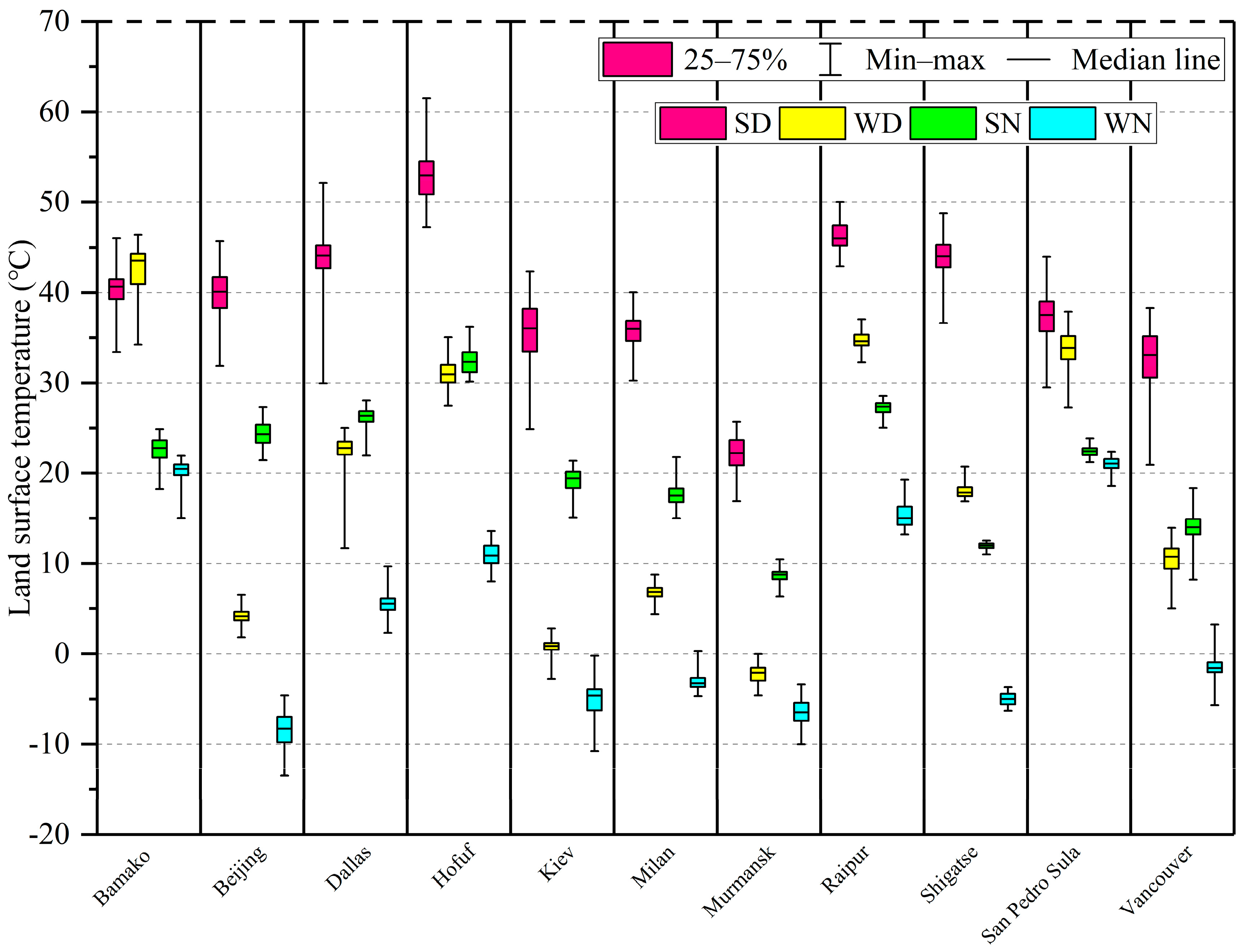
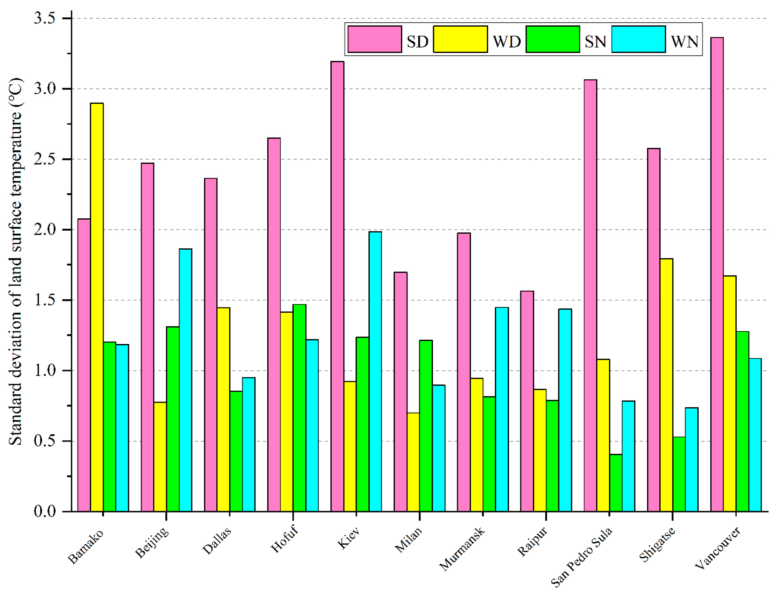
3.1. Characteristics of Land Surface Temperatures in Urban Centers in Different Climatic Zones
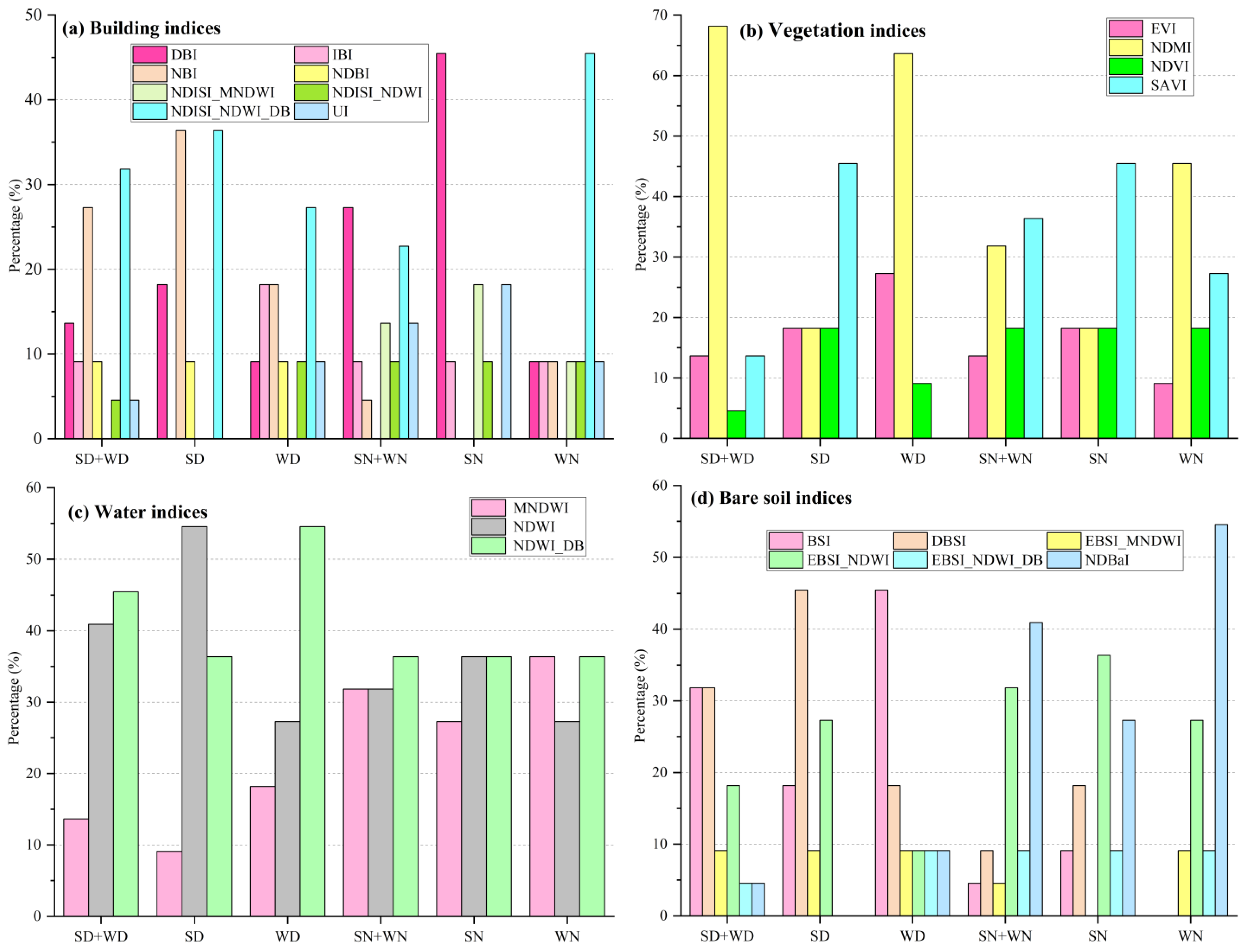
3.2. Optimal Land-Use/Land-Cover Indices of Land Surface Temperatures in Urban Centers in Different Climatic Zones
3.3. Relationships between the Optimal Land-Use/Land-Cover Indices and Land Surface Temperatures in Urban Centers in Different Global Climatic Zones
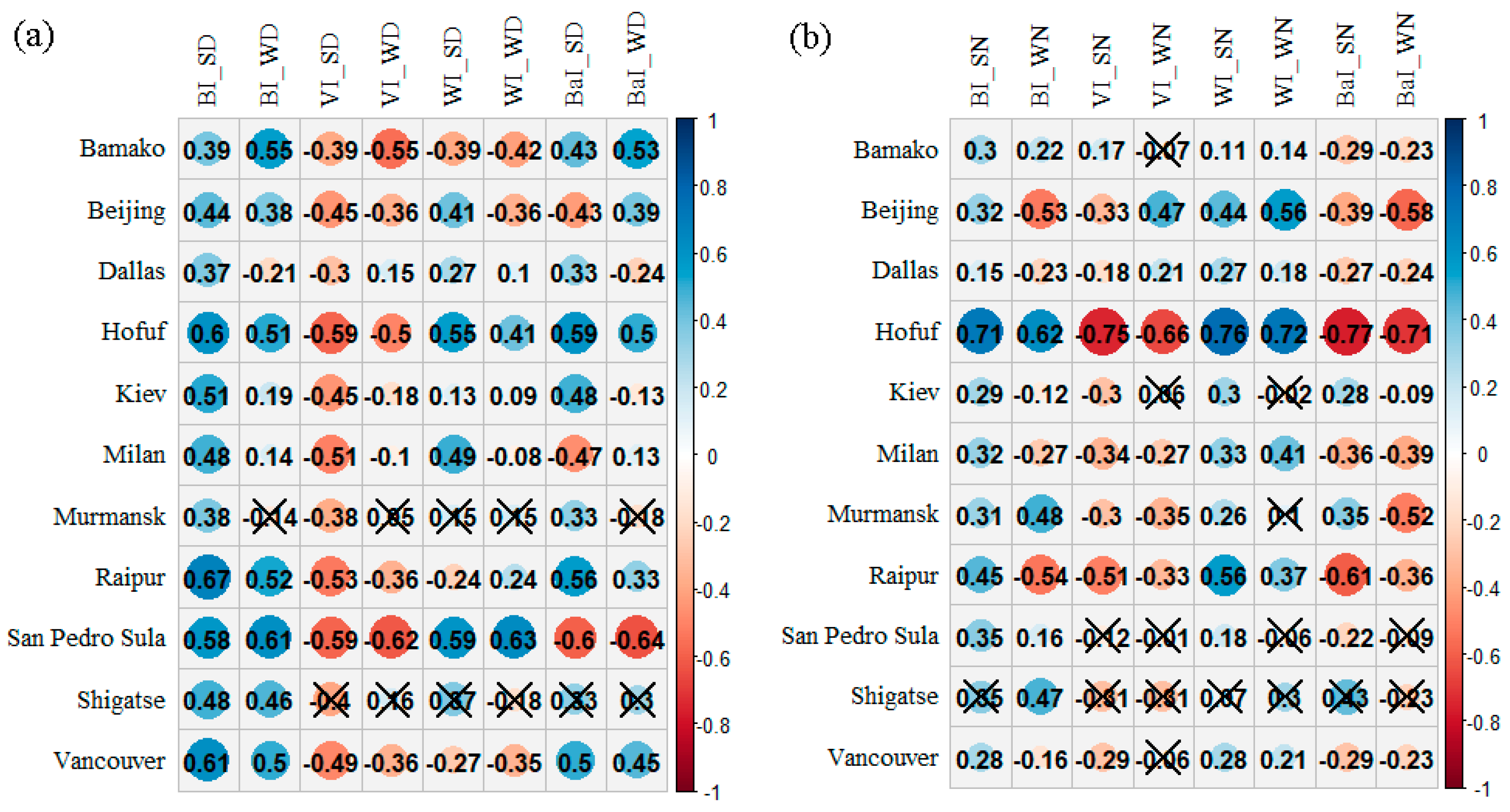
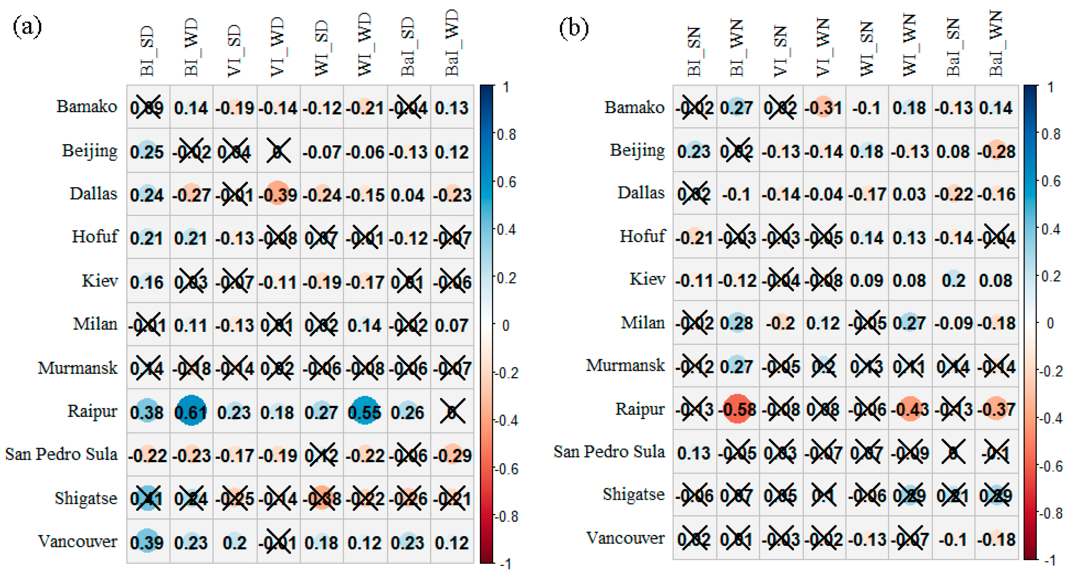
3.3.1. Relationships between the Optimal Land-Use/Land-Cover Indices and Land Surface Temperatures in Urban Centers during the Daytime
3.3.2. Relationships between Optimal Land-Use/Land-Cover Indices and Land Surface Temperatures in Urban Centers during the Nighttime
4. Discussion
4.1. Selection of the Optimal Land-Use/Land-Cover Indices of Land Surface Temperatures in Urban Centers in Different Global Climatic Zones
4.2. Influencing Mechanism of Optimal Land-Use/Land-Cover Indices on Land Surface Temperatures in Urban Centers in Different Climatic Zones
4.2.1. Building Indices
4.2.2. Vegetation Indices
4.2.3. Water Indices
4.2.4. Bare Soil Indices
4.2.5. Combined Effects
4.3. Limitations and Future Work
5. Conclusions
- (1)
- The correlation coefficients and significance levels of LU/LC indices with LSTs were quite different and even obtained opposite positive or negative relationships. NDBI, NDVI, NDWI and NDBaI were the most frequently used indices to analyze the relationships between LU/LC indices and LSTs in previous studies. Nevertheless, they were not necessarily the optimal ones under different conditions. Other indices also had high probabilities of being the optimal indices to explain LSTs, such as DBI, NBI, IBI, NDISI_NDWI_DB, NDMI, SAVI, DBSI, BSI, EBSI_NDWI, etc.
- (2)
- The daytime LSTs were generally significantly negatively with VIs and positively correlated with BIs and BaIs (p < 0.05). These relationships were usually stronger in the summer than in winter. The nighttime LSTs were generally significantly positively and negatively correlated with BIs and VIs in the summer, respectively (p < 0.05). These correlation degrees were generally lower during the nighttime than daytime, except in Hofuf. Moreover, the nighttime LSTs were significantly positively and negatively correlated with WIs and BaIs, respectively (p < 0.05).
- (3)
- Significant multiple linear regressions generally existed between the LSTs and the optimal indices of building, vegetation, water and bare soil during the daytime and nighttime (p < 0.05). The explanation rates were usually higher during the daytime than nighttime, especially in the summer. Moreover, the values of adjusted R2 of daytime LSTs were larger in the summer than in winter in most urban centers.
- (4)
- Future work may include exploring the non-linear relationships between LSTs and LU/LC indices together with the segmentation analysis, deriving laws at finer scales, considering different influences in different land uses or covers, studying the detailed mechanism by using several methods comprehensively, etc.
Supplementary Materials
Author Contributions
Funding
Data Availability Statement
Conflicts of Interest
References
- United Nations, Department of Economic and Social Affairs. World Urbanization Prospects: The 2018 Revision, Highlights; United Nations, Department of Economic and Social Affairs: New York, NY, USA, 2019. [Google Scholar]
- Asabere, S.B.; Acheampong, R.A.; Ashiagbor, G.; Beckers, S.C.; Keck, M.; Erasmi, S.; Schanze, J.; Sauer, D. Urbanization, land use transformation and spatio-environmental impacts: Analyses of trends and implications in major metropolitan regions of Ghana. Land Use Policy 2020, 96, 104707. [Google Scholar] [CrossRef]
- Wnek, A.; Kudas, D.; Stych, P. National level land-use changes in functional urban areas in Poland, Slovakia, and Czechia. Land 2021, 10, 39. [Google Scholar] [CrossRef]
- Zhou, D.; Xiao, J.; Frolking, S.; Zhang, L.; Zhou, G. Urbanization contributes little to global warming but substantially intensifies local and regional land surface warming. Earth’s Future 2022, 10, e2021EF002401. [Google Scholar] [CrossRef]
- Li, Y.; Yin, K.; Zhou, H.; Wang, X.; Hu, D. Progress in urban heat island monitoring by remote sensing. Prog. Geogr. 2016, 35, 1062–1074. [Google Scholar]
- Zha, Y.; Gao, J.; Ni, S. Use of normalized difference built-up index in automatically mapping urban areas from TM imagery. Int. J. Remote Sens. 2003, 24, 583–594. [Google Scholar] [CrossRef]
- Xu, H.; Ding, F.; Wen, X. Urban expansion and heat island dynamics in the Quanzhou region, China. IEEE J. Sel. Top. Appl. Earth Obs. Remote Sens. 2009, 2, 74–79. [Google Scholar] [CrossRef]
- Rouse, J., Jr.; Haas, R.H.; Deering, D.; Schell, J.; Harlan, J.C. Monitoring the Vernal Advancement and Retrogradation (Green Wave Effect) of Natural Vegetation; Texas A&M University: College Station, TX, USA, 1974. [Google Scholar]
- Klemas, V.; Smart, R. The influence of soil salinity, growth form, and leaf moisture on-the spectral radiance of Spartina alterniflora canopies. Photogramm. Eng. Remote Sens. 1983, 49, 77–83. [Google Scholar]
- Gao, B.-C. NDWI—A normalized difference water index for remote sensing of vegetation liquid water from space. Remote Sens. Environ. 1996, 58, 257–266. [Google Scholar] [CrossRef]
- Xu, H. Modification of normalised difference water index (NDWI) to enhance open water features in remotely sensed imagery. Int. J. Remote Sens. 2006, 27, 3025–3033. [Google Scholar] [CrossRef]
- Rikimaru, A. LAMDSAT TM data processing guide for forest canopy density mapping and monitoring model. In Proceedings of the ITTO workshop on Utilization of Remote Sensing in Site Assessment and Planning for Rehabilitation of Logged-over Forest, Bangkok, Thailand, 30 July 30–August 1 1996. [Google Scholar]
- Zhao, H.; Chen, X. Use of normalized difference bareness index in quickly mapping bare areas from TM/ETM+. In Proceedings of the International Geoscience and Remote Sensing Symposium, Seoul, Korea, 29 July 2005; p. 1666. [Google Scholar]
- Khan, M.S.; Ullah, S.; Chen, L. Comparison on land-use/land-cover indices in explaining land surface temperature variations in the city of Beijing, China. Land 2021, 10, 1018. [Google Scholar] [CrossRef]
- Guha, S.; Govil, H.; Diwan, P. Analytical study of seasonal variability in land surface temperature with normalized difference vegetation index, normalized difference water index, normalized difference built-up index, and normalized multiband drought index. J. Appl. Remote Sens. 2019, 13, 024518. [Google Scholar]
- Bonafoni, S. Spectral index utility for summer urban heating analysis. J. Appl. Remote Sens. 2015, 9, 096030. [Google Scholar] [CrossRef]
- Zhou, D.C.; Xiao, J.F.; Bonafoni, S.; Berger, C.; Deilami, K.; Zhou, Y.Y.; Frolking, S.; Yao, R.; Qiao, Z.; Sobrino, J.A. Satellite remote sensing of surface urban heat islands: Progress, challenges, and perspectives. Remote Sens. 2019, 11, 48. [Google Scholar] [CrossRef]
- Huang, J.; Fatichi, S.; Mascaro, G.; Manoli, G.; Peleg, N. Intensification of sub-daily rainfall extremes in a low-rise urban area. Urban Clim. 2022, 42, 101124. [Google Scholar] [CrossRef]
- Li, Y.; Wang, W.; Wang, Y.; Xin, Y.; He, T.; Zhao, G. A review of studies involving the effects of climate change on the energy consumption for building heating and cooling. Int. J. Environ. Res. Public Health 2021, 18, 40. [Google Scholar] [CrossRef] [PubMed]
- Weng, Q.H.; Yang, S.H. Urban air pollution patterns, land use, and thermal landscape: An examination of the linkage using GIS. Environ. Monit. Assess. 2006, 117, 463–489. [Google Scholar] [CrossRef] [PubMed]
- McGlynn, T.P.; Meineke, E.K.; Bahlai, C.A.; Li, E.J.; Hartop, E.A.; Adams, B.J.; Brown, B.V. Temperature accounts for the biodiversity of a hyperdiverse group of insects in urban Los Angeles. Proc. R. Soc. B Biol. Sci. 2019, 286, 20191818. [Google Scholar] [CrossRef]
- Li, J.; Sun, R.; Liu, T.; Xie, W.; Chen, L. Prediction models of urban heat island based on landscape patterns and anthropogenic heat dynamics. Landsc. Ecol. 2021, 36, 1801–1815. [Google Scholar] [CrossRef]
- Yang, G.; Pu, R.; Zhao, C.; Huang, W.; Wang, J. Estimation of subpixel land surface temperature using an endmember index based technique: A case examination on ASTER and MODIS temperature products over a heterogeneous area. Remote Sens. Environ. 2011, 115, 1202–1219. [Google Scholar] [CrossRef]
- Chen, X.; Zhao, H.; Li, P.; Yin, Z. Remote sensing image-based analysis of the relationship between urban heat island and land use/cover changes. Remote Sens. Environ. 2006, 104, 133–146. [Google Scholar] [CrossRef]
- Zhang, Y.; Odeh, I.O.; Han, C. Bi-temporal characterization of land surface temperature in relation to impervious surface area, NDVI and NDBI, using a sub-pixel image analysis. Int. J. Appl. Earth Obs. Geoinf. 2009, 11, 256–264. [Google Scholar] [CrossRef]
- Siqi, J.; Yuhong, W. Effects of land use and land cover pattern on urban temperature variations: A case study in Hong Kong. Urban Clim. 2020, 34, 100693. [Google Scholar] [CrossRef]
- Tetali, S.; Baird, N.; Klima, K. A multicity analysis of daytime surface urban heat islands in India and the US. Sustain. Cities Soc. 2022, 77, 103568. [Google Scholar] [CrossRef]
- Shinkarenko, S.; Kosheleva, O.Y.; Gordienko, O.; Dubacheva, A.; Omarov, R. The relationship between the seasonal dynamics of surface temperature and NDVI in urbanized areas of an arid zone. The case of the Volgograd agglomeration. Izv. Atmos. Ocean. Phys. 2021, 57, 1576–1585. [Google Scholar] [CrossRef]
- Bala, R.; Prasad, R.; Yadav, V.P. A comparative analysis of day and night land surface temperature in two semi-arid cities using satellite images sampled in different seasons. Adv. Space Res. 2020, 66, 412–425. [Google Scholar] [CrossRef]
- Bindajam, A.A.; Mallick, J.; AlQadhi, S.; Singh, C.K.; Hang, H.T. Impacts of vegetation and topography on land surface temperature variability over the semi-arid mountain cities of Saudi Arabia. Atmosphere 2020, 11, 762. [Google Scholar] [CrossRef]
- Huang, C.; Ye, X. Spatial modeling of urban vegetation and land surface temperature: A case study of Beijing. Sustainability 2015, 7, 9478–9504. [Google Scholar] [CrossRef]
- Liu, L.; Zhang, Y. Urban heat island analysis using the Landsat TM data and ASTER data: A case study in Hong Kong. Remote Sens. 2011, 3, 1535–1552. [Google Scholar] [CrossRef]
- Kant, Y.; Bharath, B.; Mallick, J.; Atzberger, C.; Kerle, N. Satellite-based analysis of the role of land use/land cover and vegetation density on surface temperature regime of Delhi, India. J. Indian Soc. Remote Sens. 2009, 37, 201–214. [Google Scholar] [CrossRef]
- Sannigrahi, S.; Bhatt, S.; Rahmat, S.; Uniyal, B.; Banerjee, S.; Chakraborti, S.; Jha, S.; Lahiri, S.; Santra, K.; Bhatt, A. Analyzing the role of biophysical compositions in minimizing urban land surface temperature and urban heating. Urban Clim. 2018, 24, 803–819. [Google Scholar] [CrossRef]
- Guha, S.; Govil, H. A long-term monthly analytical study on the relationship of LST with normalized difference spectral indices. Eur. J. Remote Sens. 2021, 54, 487–512. [Google Scholar] [CrossRef]
- Meng, X.; Meng, F.; Zhao, Z.; Yin, C. Prediction of urban heat island effect over Jinan City using the markov-cellular automata model combined with urban biophysical descriptors. J. Indian Soc. Remote Sens. 2021, 49, 997–1009. [Google Scholar] [CrossRef]
- Chen, L.; Wang, X.; Cai, X.; Yang, C.; Lu, X. Seasonal variations of daytime land surface temperature and their underlying drivers over Wuhan, China. Remote Sens. 2021, 13, 323. [Google Scholar] [CrossRef]
- Guha, S.; Govil, H. Seasonal impact on the relationship between land surface temperature and normalized difference vegetation index in an urban landscape. Geocarto Int. 2020, 37, 2252–2272. [Google Scholar] [CrossRef]
- Sekertekin, A.; Zadbagher, E. Simulation of future land surface temperature distribution and evaluating surface urban heat island based on impervious surface area. Ecol. Indic. 2021, 122, 107230. [Google Scholar] [CrossRef]
- Zhao, X.; Liu, J.; Bu, Y. Quantitative analysis of spatial heterogeneity and driving forces of the thermal environment in urban built-up areas: A case study in Xi’an, China. Sustainability 2021, 13, 1870. [Google Scholar] [CrossRef]
- Alibakhshi, Z.; Ahmadi, M.; Farajzadeh Asl, M. Modeling biophysical variables and land surface temperature using the GWR model: Case study—Tehran and its satellite cities. J. Indian Soc. Remote Sens. 2020, 48, 59–70. [Google Scholar] [CrossRef]
- Mathew, A.; Khandelwal, S.; Kaul, N. Investigating spatial and seasonal variations of urban heat island effect over Jaipur city and its relationship with vegetation, urbanization and elevation parameters. Sustain. Cities Soc. 2017, 35, 157–177. [Google Scholar] [CrossRef]
- Sahana, M.; Dutta, S.; Sajjad, H. Assessing land transformation and its relation with land surface temperature in Mumbai city, India using geospatial techniques. Int. J. Urban Sci. 2019, 23, 205–225. [Google Scholar] [CrossRef]
- Renard, F.; Alonso, L.; Fitts, Y.; Hadjiosif, A.; Comby, J. Evaluation of the effect of urban redevelopment on surface urban heat islands. Remote Sens. 2019, 11, 299. [Google Scholar] [CrossRef]
- Rihan, M.; Naikoo, M.W.; Ali, M.A.; Usmani, T.M.; Rahman, A. Urban heat island dynamics in response to land-use/land-cover change in the coastal city of Mumbai. J. Indian Soc. Remote Sens. 2021, 49, 2227–2247. [Google Scholar]
- Hashim, B.M.; Al Maliki, A.; Sultan, M.A.; Shahid, S.; Yaseen, Z.M. Effect of land use land cover changes on land surface temperature during 1984–2020: A case study of Baghdad city using landsat image. Nat. Hazards 2022, 112, 1223–1246. [Google Scholar] [CrossRef]
- Hasan, M.; Hassan, L.; Al, M.A.; Abualreesh, M.H.; Idris, M.H.; Kamal, A.H.M. Urban green space mediates spatiotemporal variation in land surface temperature: A case study of an urbanized city, Bangladesh. Environ. Sci. Pollut. Res. 2022, 29, 36376–36391. [Google Scholar] [CrossRef] [PubMed]
- Edan, M.H.; Maarouf, R.M.; Hasson, J. Predicting the impacts of land use/land cover change on land surface temperature using remote sensing approach in Al Kut, Iraq. Phys. Chem. Earth Parts A/B/C 2021, 123, 103012. [Google Scholar] [CrossRef]
- Koko, A.F.; Wu, Y.; Abubakar, G.A.; Alabsi, A.A.N.; Hamed, R.; Bello, M. Thirty years of land use/land cover changes and their impact on urban climate: A study of Kano metropolis, Nigeria. Land 2021, 10, 1106. [Google Scholar] [CrossRef]
- Mudede, M.F.; Newete, S.W.; Abutaleb, K.; Nkongolo, N. Monitoring the urban environment quality in the city of Johannesburg using remote sensing data. J. Afr. Earth Sci. 2020, 171, 103969. [Google Scholar] [CrossRef]
- Choudhury, D.; Das, K.; Das, A. Assessment of land use land cover changes and its impact on variations of land surface temperature in Asansol-Durgapur Development Region. Egypt. J. Remote Sens. Space Sci. 2019, 22, 203–218. [Google Scholar] [CrossRef]
- Xiong, Y.; Huang, S.; Chen, F.; Ye, H.; Wang, C.; Zhu, C. The impacts of rapid urbanization on the thermal environment: A remote sensing study of Guangzhou, South China. Remote Sens. 2012, 4, 2033–2056. [Google Scholar] [CrossRef]
- Mondal, A.; Guha, S.; Kundu, S. Dynamic status of land surface temperature and spectral indices in Imphal city, India from 1991 to 2021. Geomat. Nat. Hazards Risk 2021, 12, 3265–3286. [Google Scholar] [CrossRef]
- Verma, R.; Garg, P.K. Mapping the spatiotemporal changes of land use/land cover on the urban heat island effect by open source data: A case study of Lucknow, India. J. Indian Soc. Remote Sens. 2021, 49, 2655–2671. [Google Scholar] [CrossRef]
- Yang, Z.; Witharana, C.; Hurd, J.; Wang, K.; Hao, R.; Tong, S. Using Landsat 8 data to compare percent impervious surface area and normalized difference vegetation index as indicators of urban heat island effects in Connecticut, USA. Environ. Earth Sci. 2020, 79, 1–13. [Google Scholar] [CrossRef]
- Guha, S.; Govil, H.; Dey, A.; Gill, N. Analytical study of land surface temperature with NDVI and NDBI using Landsat 8 OLI and TIRS data in Florence and Naples city, Italy. Eur. J. Remote Sens. 2018, 51, 667–678. [Google Scholar] [CrossRef]
- Sarfo, I.; Shuoben, B.; Beibei, L.; Amankwah, S.O.Y.; Yeboah, E.; Koku, J.E.; Nunoo, E.K.; Kwang, C. Spatiotemporal development of land use systems, influences and climate variability in Southwestern Ghana (1970–2020). Environ. Dev. Sustain. 2021, 24, 9851–9883. [Google Scholar] [CrossRef]
- Koko, A.F.; Yue, W.; Abubakar, G.A.; Alabsi, A.A.N.; Hamed, R. Spatiotemporal influence of land use/land cover change dynamics on surface urban heat island: A case study of Abuja metropolis, Nigeria. ISPRS Int. J. Geo-Inf. 2021, 10, 272. [Google Scholar] [CrossRef]
- Ranagalage, M.; Estoque, R.C.; Murayama, Y. An urban heat island study of the Colombo metropolitan area, Sri Lanka, based on Landsat data (1997–2017). ISPRS Int. J. Geo-Inf. 2017, 6, 189. [Google Scholar] [CrossRef]
- Khan, R.; Li, H.; Basir, M.; Chen, Y.L.; Sajjad, M.M.; Haq, I.U.; Ullah, B.; Arif, M.; Hassan, W. Monitoring land use land cover changes and its impacts on land surface temperature over Mardan and Charsadda Districts, Khyber Pakhtunkhwa (KP), Pakistan. Environ. Monit. Assess. 2022, 194, 1–22. [Google Scholar] [CrossRef]
- Hua, A.K.; Ping, O.W. The influence of land-use/land-cover changes on land surface temperature: A case study of Kuala Lumpur metropolitan city. Eur. J. Remote Sens. 2018, 51, 1049–1069. [Google Scholar] [CrossRef]
- Aslam, A.; Rana, I.A.; Bhatti, S.S. The spatiotemporal dynamics of urbanisation and local climate: A case study of Islamabad, Pakistan. Environ. Impact Assess. Rev. 2021, 91, 106666. [Google Scholar] [CrossRef]
- Bektaş Balçik, F. Determining the impact of urban components on land surface temperature of Istanbul by using remote sensing indices. Environ. Monit. Assess. 2014, 186, 859–872. [Google Scholar] [CrossRef]
- Ma, X.; Peng, S. Research on the spatiotemporal coupling relationships between land use/land cover compositions or patterns and the surface urban heat island effect. Environ. Sci. Pollut. Res. 2022, 29, 39723–39742. [Google Scholar] [CrossRef]
- Guo, G.; Wu, Z.; Xiao, R.; Chen, Y.; Liu, X.; Zhang, X. Impacts of urban biophysical composition on land surface temperature in urban heat island clusters. Landsc. Urban Plan. 2015, 135, 1–10. [Google Scholar] [CrossRef]
- Wan, Z. New refinements and validation of the MODIS land-surface temperature/emissivity products. Remote Sens. Environ. 2008, 112, 59–74. [Google Scholar] [CrossRef]
- Rigo, G.; Parlow, E.; Oesch, D. Validation of satellite observed thermal emission with in-situ measurements over an urban surface. Remote Sens. Environ. 2006, 104, 201–210. [Google Scholar] [CrossRef]
- Clinton, N.; Gong, P. MODIS detected surface urban heat islands and sinks: Global locations and controls. Remote Sens. Environ. 2013, 134, 294–304. [Google Scholar] [CrossRef]
- Li, Y.; Feng, Z.; Li, L.; Li, T.; Guo, F.; Wei, J.; Yan, Y.; Wang, L. Surface urban heat islands in 932 urban region agglomerations in China during the morning and before midnight: Spatial-temporal changes, drivers, and simulation. Geocarto Int. 2022, 1–19. [Google Scholar] [CrossRef]
- Yoo, C.; Im, J.; Cho, D.; Lee, Y.; Bae, D.; Sismanidis, P. Downscaling MODIS nighttime land surface temperatures in urban areas using ASTER thermal data through local linear forest. Int. J. Appl. Earth Obs. Geoinf. 2022, 110, 102827. [Google Scholar] [CrossRef]
- Sismanidis, P.; Bechtel, B.; Perry, M.; Ghent, D. The Seasonality of Surface Urban Heat Islands across Climates. Remote Sens. 2022, 14, 2318. [Google Scholar] [CrossRef]
- Florczyk, A.E.A.; Florczyk, A.; Corbane, C.; Schiavina, M.; Pesaresi, M.; Maffenini, L.; Melchiorri, M.; Politis, P.; Sabo, F.; Freire, S.; et al. GHS Urban Centre Database 2015, Multitemporal and Multidimensional Attributes, R2019A. European Commission, Joint Research Centre (JRC) [Dataset] PID. 2019. Available online: https://data.jrc.ec.europa.eu/dataset/53473144-b88c-44bc-b4a3-4583ed1f547e (accessed on 8 February 2022).
- Lloyd, C.T.; Sorichetta, A.; Tatem, A.J. High resolution global gridded data for use in population studies. Sci. Data 2017, 4, 170001. [Google Scholar] [CrossRef]
- Wang, Y.C.; Huang, C.L.; Zhao, M.Y.; Hou, J.L.; Zhang, Y.; Gu, J. Mapping the population density in mainland China using NPP/VIIRS and points-of-interest data based on a random forests model. Remote Sens. 2020, 12, 3645. [Google Scholar] [CrossRef]
- Mohanty, M.P.; Simonovic, S.P. Understanding dynamics of population flood exposure in Canada with multiple high-resolution population datasets. Sci. Total Environ. 2021, 759, 143559. [Google Scholar] [CrossRef]
- Estoque, R.C.; Murayama, Y.; Myint, S.W. Effects of landscape composition and pattern on land surface temperature: An urban heat island study in the megacities of Southeast Asia. Sci. Total Environ. 2017, 577, 349–359. [Google Scholar] [CrossRef] [PubMed]
- Bokaie, M.; Zarkesh, M.K.; Arasteh, P.D.; Hosseini, A. Assessment of urban heat island based on the relationship between land surface temperature and land use/land cover in Tehran. Sustain. Cities Soc. 2016, 23, 94–104. [Google Scholar] [CrossRef]
- Rasul, A.; Balzter, H.; Ibrahim, G.R.F.; Hameed, H.M.; Wheeler, J.; Adamu, B.; Ibrahim, S.a.; Najmaddin, P.M. Applying built-up and bare-soil indices from Landsat 8 to cities in dry climates. Land 2018, 7, 81. [Google Scholar] [CrossRef]
- Chen, J.; Liu, Y.; Li, M.; Shen, C.; Hu, W.; Cai, W. A new method of extracting residential areas based on remote sensing image. Geogr. Geo-Inf. Sci. 2010, 26, 72–75, 113. [Google Scholar]
- Xu, H. A new remote sensing index for fastly extracting impervious surface information. Geomat. Inf. Sci. Wuhan Univ. 2008, 33, 1150–1153, 1211. [Google Scholar]
- Kawamura, M.; Jayamana, S.; Tsujiko, Y. Relation between social and environmental conditions in Colombo Sri Lanka and the urban index estimated by satellite remote sensing data. Int. Soc. Photogramm. Remote. Sens. 1996, 31, 321–326. [Google Scholar]
- Liu, H.Q.; Huete, A. A feedback based modification of the NDVI to minimize canopy background and atmospheric noise. IEEE Trans. Geosci. Remote Sens. 1995, 33, 457–465. [Google Scholar] [CrossRef]
- Huete, A.R. A soil-adjusted vegetation index (SAVI). Remote Sens. Environ. 1988, 25, 295–309. [Google Scholar] [CrossRef]
- Li, Y.; Gong, X.; Guo, Z.; Xu, K.; Hu, D.; Zhou, H. An index and approach for water extraction using Landsat-OLI data. Int. J. Remote Sens. 2016, 37, 3611–3635. [Google Scholar] [CrossRef]
- Wu, Z.; Zhao, S. A study of enhanced index-based built-up index based on Landsat TM imagery. Remote Sens. Land Resour. 2012, 24, 50–55. [Google Scholar]
- As-syakur, A.; Adnyana, I.W.S.; Mahendra, M.S.; Arthana, I.W.; Merit, I.N.; Kasa, I.W.; Ekayanti, N.W.; Nuarsa, I.W.; Sunarta, I.N. Observation of spatial patterns on the rainfall response to ENSO and IOD over Indonesia using TRMM Multisatellite Precipitation Analysis (TMPA). Int. J. Climatol. 2014, 34, 3825–3839. [Google Scholar] [CrossRef]
- Song, Z.; Li, R.; Qiu, R.; Liu, S.; Tan, C.; Li, Q.; Ge, W.; Han, X.; Tang, X.; Shi, W. Global land surface temperature influenced by vegetation cover and PM2. 5 from 2001 to 2016. Remote Sens. 2018, 10, 2034. [Google Scholar] [CrossRef]
- Li, X.Y.; He, X.F.; Pan, X. Application of Gaofen-6 images in the downscaling of land surface temperatures. Remote Sens. 2022, 14, 2307. [Google Scholar] [CrossRef]
- Xiao, Z.X.; Wang, Z.Q.; Pan, W.J.; Wang, Y.L.; Yang, S. Sensitivity of extreme temperature events to urbanization in the Pearl River Delta Region. Asia Pac. J. Atmos. Sci. 2019, 55, 373–386. [Google Scholar] [CrossRef]
- Liu, X.J.; Tian, G.J.; Feng, J.M.; Ma, B.R.; Wang, J.; Kong, L.Q. Modeling the warming impact of urban land expansion on hot weather using the weather research and forecasting model: A case study of Beijing, China. Adv. Atmos. Sci. 2018, 35, 723–736. [Google Scholar] [CrossRef]
- Yamak, B.; Yagci, Z.; Bilgilioglu, B.B.; Comert, R. Investigation of the effect of urbanization on land surface temperature example of Bursa. Int. J. Eng. Geosci. 2021, 6, 1–8. [Google Scholar] [CrossRef]
- Oke, T.R. The energetic basis of the urban heat island. Q. J. R. Meteorol. Soc. 1982, 108, 1–24. [Google Scholar] [CrossRef]
- Park, Y.J.; Guldmann, J.M.; Liu, D.S. Impacts of tree and building shades on the urban heat island: Combining remote sensing, 3D digital city and spatial regression approaches. Comput. Environ. Urban Syst. 2021, 88, 101655. [Google Scholar] [CrossRef]
- Zhang, Y.; Sun, L. Spatial-temporal impacts of urban land use land cover on land surface temperature: Case studies of two Canadian urban areas. Int. J. Appl. Earth Obs. Geoinf. 2019, 75, 171–181. [Google Scholar] [CrossRef]
- Chen, X.; Zhang, Y. Impacts of urban surface characteristics on spatiotemporal pattern of land surface temperature in Kunming of China. Sustain. Cities Soc. 2017, 32, 87–99. [Google Scholar] [CrossRef]
- Neog, R. Evaluation of temporal dynamics of land use and land surface temperature (LST) in Agartala city of India. Environ. Dev. Sustain. 2022, 24, 3419–3438. [Google Scholar] [CrossRef]
- Biswas, S.; Ghosh, S. Estimation of land surface temperature in response to land use/land cover transformation in Kolkata city and its suburban area, India. Int. J. Urban Sci. 2021, 1–28. [Google Scholar] [CrossRef]
- Li, Y.; Wang, L.; Zhang, L.; Liu, M.; Zhao, G. Monitoring intra-annual spatiotemporal changes in urban heat islands in 1449 cities in China based on remote sensing. Chin. Geogr. Sci. 2019, 29, 905–916. [Google Scholar] [CrossRef]
- Kato, S.; Yamaguchi, Y. Estimation of storage heat flux in an urban area using ASTER data. Remote Sens. Environ. 2007, 110, 1–17. [Google Scholar] [CrossRef]
- Marando, F.; Heris, M.P.; Zulian, G.; Udias, A.; Mentaschi, L.; Chrysoulakis, N.; Parastatidis, D.; Maes, J. Urban heat island mitigation by green infrastructure in European functional urban areas. Sustain. Cities Soc. 2022, 77, 103564. [Google Scholar] [CrossRef]
- Schultz, N.M.; Lawrence, P.J.; Lee, X. Global satellite data highlights the diurnal asymmetry of the surface temperature response to deforestation. J. Geophys. Res. Biogeosci. 2017, 122, 903–917. [Google Scholar] [CrossRef]
- Wang, C.H.; Wang, Z.H.; Wang, C.Y.; Myint, S.W. Environmental cooling provided by urban trees under extreme heat and cold waves in US cities. Remote Sens. Environ. 2019, 227, 28–43. [Google Scholar] [CrossRef]
- Chen, T. Studies on Spatiotemporal Dynamics of Thermal Radiation Temperatures of Different Landscapes In Beijing City; University of Science and Technology of China: Hefei, China, 2017. [Google Scholar]
- Chudnovsky, A.; Ben-Dor, E.; Saaroni, H. Diurnal thermal behavior of selected urban objects using remote sensing measurements. Energy Build. 2004, 36, 1063–1074. [Google Scholar] [CrossRef]
- Kim, H.H. Urban heat island. Int. J. Remote Sens. 1992, 13, 2319–2336. [Google Scholar] [CrossRef]
- Ossola, A.; Jenerette, G.D.; McGrath, A.; Chow, W.; Hughes, L.; Leishman, M.R. Small vegetated patches greatly reduce urban surface temperature during a summer heatwave in Adelaide, Australia. Landsc. Urban Plan. 2021, 209, 104046. [Google Scholar] [CrossRef]
- Yu, Q.Y.; Ji, W.J.; Pu, R.L.; Landry, S.; Acheampong, M.; O’Neil-Dunne, J.; Ren, Z.B.; Tanim, S.H. A preliminary exploration of the cooling effect of tree shade in urban landscapes. Int. J. Appl. Earth Obs. Geoinf. 2020, 92, 102161. [Google Scholar] [CrossRef]
- Upreti, R.; Wang, Z.H.; Yang, J.C. Radiative shading effect of urban trees on cooling the regional built environment. Urban For. Urban Green 2017, 26, 18–24. [Google Scholar] [CrossRef]
- Quan, J.; Zhan, W.; Chen, Y.; Wang, M.; Wang, J. Time series decomposition of remotely sensed land surface temperature and investigation of trends and seasonal variations in surface urban heat islands. J. Geophys. Res. Atmos. 2016, 121, 2638–2657. [Google Scholar] [CrossRef]
- Rahaman, S.; Kumar, P.; Chen, R.; Meadows, M.E.; Singh, R. Remote sensing assessment of the impact of land use and land cover change on the environment of Barddhaman district, West Bengal, India. Front. Environ. Sci. 2020, 8, 127. [Google Scholar] [CrossRef]
- Guha, S.; Govil, H.; Dey, A.; Gill, N. A case study on the relationship between land surface temperature and land surface indices in Raipur City, India. Geogr. Tidsskr. -Dan. J. Geogr. 2020, 120, 35–50. [Google Scholar] [CrossRef]
- Offerle, B.; Jonsson, P.; Eliasson, I.; Grimmond, C. Urban modification of the surface energy balance in the West African Sahel: Ouagadougou, Burkina Faso. J. Clim. 2005, 18, 3983–3995. [Google Scholar] [CrossRef]
- Rahman, M.T.; Aldosary, A.S.; Mortoja, M.G. Modeling future land cover changes and their effects on the land surface temperatures in the Saudi Arabian eastern coastal city of Dammam. Land 2017, 6, 36. [Google Scholar] [CrossRef]
- Buo, I.; Sagris, V.; Burdun, I.; Uuemaa, E. Estimating the expansion of urban areas and urban heat islands (UHI) in Ghana: A case study. Nat. Hazards 2021, 105, 1299–1321. [Google Scholar] [CrossRef]
- Ullah, S.; Tahir, A.A.; Akbar, T.A.; Hassan, Q.K.; Dewan, A.; Khan, A.J.; Khan, M. Remote sensing-based quantification of the relationships between land use land cover changes and surface temperature over the Lower Himalayan Region. Sustainability 2019, 11, 5492. [Google Scholar] [CrossRef]
- Guha, S.; Govil, H. An assessment on the relationship between land surface temperature and normalized difference vegetation index. Environ. Dev. Sustain. 2021, 23, 1944–1963. [Google Scholar] [CrossRef]
- Siddiqui, A.; Kushwaha, G.; Raoof, A.; Verma, P.A.; Kant, Y. Bangalore: Urban heating or urban cooling? Egypt. J. Remote Sens. Space Sci. 2021, 24, 265–272. [Google Scholar] [CrossRef]
- Chang, Y.; Xiao, J.; Li, X.; Middel, A.; Zhang, Y.; Gu, Z.; Wu, Y.; He, S. Exploring diurnal thermal variations in urban local climate zones with ECOSTRESS land surface temperature data. Remote Sens. Environ. 2021, 263, 112544. [Google Scholar] [CrossRef]
- Feng, L.; Tian, H.H.; Qiao, Z.; Zhao, M.M.; Liu, Y.X. Detailed variations in urban surface temperatures exploration based on unmanned aerial vehicle thermography. IEEE J. Sel. Top. Appl. Earth Obs. Remote Sens. 2020, 13, 204–216. [Google Scholar] [CrossRef]
- Tattersall, G.J.; Danner, R.M.; Chaves, J.A.; Levesque, D.L. Activity analysis of thermal imaging videos using a difference imaging approach. J. Therm. Biol. 2020, 91, 102611. [Google Scholar] [CrossRef]
- Luo, X.; Li, W. Scale effect analysis of the relationships between urban heat island and impact factors: Case study in Chongqing. J. Appl. Remote Sens. 2014, 8, 084995. [Google Scholar] [CrossRef]
- Padmanaban, R.; Bhowmik, A.K.; Cabral, P. Satellite image fusion to detect changing surface permeability and emerging urban heat islands in a fast-growing city. PLoS ONE 2019, 14, e0208949. [Google Scholar] [CrossRef] [PubMed]

| City | Country | Climatic Zone | Urban Area Size in 2015 (km2) | Total Population in 2020 (Thousand) | Population Density in 2020 (People × km−2) | Barycentric Coordinate |
|---|---|---|---|---|---|---|
| Bamako | Mali | Tropical savanna | 330 | 3446 | 10,442 | 12.62° N, 7.98° W |
| Beijing | China | Temperate monsoon | 2111 | 14,349 | 6797 | 39.90° N, 116.35° E |
| Dallas | United States | Subtropical monsoon | 5867 | 4850 | 819 | 32.86° N, 96.96° W |
| Hofuf | Saudi Arabia | Tropical desert | 269 | 2440 | 9071 | 25.41° N, 49.63° E |
| Kiev | Ukraine | Temperate continental | 519 | 166 | 319 | 50.44° N, 30.52° E |
| Milan | Italy | Mediterranean | 753 | 1863 | 2474 | 45.54° N, 9.19° E |
| Murmansk | Russia | Polar | 72 | 71 | 992 | 68.96° N, 33.08° E |
| Raipur | India | Tropical monsoon | 642 | 5612 | 8741 | 21.26° N, 81.62° E |
| San Pedro Sula | Honduras | Tropical rainy | 199 | 346 | 1741 | 15.50° N, 87.98° W |
| Shigatse | China | Alpine | 18 | 53 | 2965 | 29.26° N, 88.89° E |
| Vancouver | Canada | Temperature marine | 698 | 1551 | 2223 | 49.23° N, 122.99° W |
| Season | City | Aqua/MODIS | Landsat/OLI |
|---|---|---|---|
| Summer | Bamako | MYD11A2.A2021153.h17v07.061.2021162060303.hdf | LC08_L1TP_199051_20210607_20210615_02_T1 |
| Beijing | MYD11A2.A2017185.h26v04.061.2021307195911.hdf, MYD11A2.A2017185.h26v05.061.2021307195911.hdf | LC08_L1TP_123032_20170710_20200903_02_T1 | |
| Dallas | MYD11A2.A2015201.h09v05.061.2021359214832.hdf | LC08_L1TP_027037_20150720_20200909_02_T1 | |
| Hofuf | MYD11A2.A2021201.h22v06.061.2021210062753.hdf | LC08_L1TP_164042_20210720_20210729_02_T1 | |
| Kiev | MYD11A2.A2016193.h19v03.061.2022017092925.hdf | LC08_L1TP_181025_20160713_20200906_02_T1 | |
| Milan | MYD11A2.A2016233.h18v04.061.2022019014701.hdf | LC08_L1TP_194028_20160825_20200906_02_T1 | |
| Murmansk | MYD11A2.A2021177.h19v02.061.2021188140407.hdf | LC08_L1TP_189011_20210703_20210712_02_T1 | |
| Raipur | MYD11A2.A2014153.h25v06.061.2021334075503.hdf | LC08_L1TP_142045_20140605_20200911_02_T1 | |
| San Pedro Sula | MYD11A2.A2017233.h09v07.061.2021309102328.hdf | LC08_L1TP_018049_20170827_20200903_02_T1 | |
| Shigatse | MYD11A2.A2019161.h25v06.061.2020354210223.hdf | LC08_L1TP_139040_20190614_20200828_02_T1 | |
| Vancouver | MYD11A2.A2020225.h09v04.061.2021014061238.hdf | LC08_L1TP_047026_20200814_20210330_02_T1 | |
| Winter | Bamako | MYD11A2.A2021025.h17v07.061.2021042222603.hdf | LC08_L1TP_199051_20210130_20210302_02_T1 |
| Beijing | MYD11A2.A2022009.h26v04.061.2022018191611.hdf, MYD11A2.A2022009.h26v05.061.2022018191307.hdf | LC08_L1TP_123032_20220113_20220123_02_T1 | |
| Dallas | MYD11A2.A2016025.h09v05.061.2022003114136.hdf | LC08_L1TP_027037_20160128_20200907_02_T1 | |
| Hofuf | MYD11A2.A2021025.h22v06.061.2021042223127.hdf | LC08_L1TP_164042_20210125_20210305_02_T1 | |
| Kiev | MYD11A2.A2018001.h19v03.061.2021316074352.hdf | LC08_L1TP_181025_20180108_20200902_02_T1 | |
| Milan | MYD11A2.A2021009.h18v04.061.2021041054240.hdf | LC08_L1TP_194028_20210111_20210307_02_T1 | |
| Murmansk | MYD11A2.A2022073.h19v02.061.2022082060619.hdf | LC08_L1TP_189011_20220316_20220316_02_RT | |
| Raipur | MYD11A2.A2021009.h25v06.061.2021041053541.hdf | LC08_L1TP_142045_20210115_20210308_02_T1 | |
| San Pedro Sula | MYD11A2.A2021025.h09v07.061.2021042222552.hdf | LC08_L1TP_018049_20210126_20210305_02_T1 | |
| Shigatse | MYD11A2.A2021009.h25v06.061.2021041053541.hdf | LC08_L1TP_139040_20210110_20210307_02_T1 | |
| Vancouver | MYD11A2.A2020049.h09v04.061.2021006162447.hdf | LC08_L1TP_047026_20200220_20200822_02_T1 |
| Category | Acronym | Full Name | Equation | Reference |
|---|---|---|---|---|
| Building indices | DBI | Dry built-up index | [78] | |
| IBI | Index-based built-up index | [7] | ||
| NBI | New built-up index | [79] | ||
| NDBI | Normalized difference building index | [6] | ||
| NDISI_ MNDWI | Normalized difference impervious surface index based on MNDWI | [80] | ||
| NDISI_NDWI | Normalized difference impervious surface index based on NDWI | |||
| NDISI_NDWI_DB | Normalized difference impervious surface index based on NDWI_DB | |||
| UI | Urban index | [81] | ||
| Vegetation indices | EVI | Enhanced vegetation index | [82] | |
| NDMI | Normalized different moisture index | [9] | ||
| NDVI | Normalized vegetation index | [8] | ||
| SAVI | Soil-regulating vegetation index | [83] | ||
| Water indices | MNDWI | Modified normalized water index | [11] | |
| NDWI | Normalized difference water index | [10] | ||
| NDWI_DB | Normalized difference water index based on dark blue band | [84] | ||
| Bare soil indices | BSI | Bare soil index | [12] | |
| DBSI | Dry bare soil index | [78] | ||
| EBSI_MNDWI | Enhanced bare soil index based on MNDWI | [85] | ||
| EBSI_NDWI | Enhanced bare soil index based on NDWI | |||
| EBSI_NDWI_DB | Enhanced bare soil index based on NDWI_DB | |||
| NDBaI | Normalized difference bare soil index | [13] |
| Time | City | Building Index | Vegetation Index | Water Index | Bare Soil Index |
|---|---|---|---|---|---|
| SD | Bamako | NDISI_NDWI_DB | NDMI | NDWI_DB | EBSI_MNDWI |
| Beijing | NDISI_NDWI_DB | SAVI | MNDWI | EBSI_NDWI | |
| Dallas | NBI | NDMI | NDWI | DBSI | |
| Hofuf | NBI | NDMI | NDWI | BSI | |
| Kiev | NBI | NDMI | NDWI | DBSI | |
| Milan | DBI | SAVI | NDWI | EBSI_NDWI | |
| Murmansk | NDBI | NDMI | NDWI_DB | BSI | |
| Raipur | NDISI_NDWI_DB | NDMI | NDWI_DB | DBSI | |
| San Pedro Sula | DBI | SAVI | NDWI | EBSI_NDWI | |
| Shigatse | NBI | NDMI | NDWI | DBSI | |
| Vancouver | NDISI_NDWI_DB | NDMI | NDWI_DB | DBSI | |
| WD | Bamako | NDBI | NDMI | NDWI_DB | DBSI |
| Beijing | IBI | NDMI | NDWI_DB | BSI | |
| Dallas | IBI | NDMI | NDWI_DB | BSI | |
| Hofuf | NBI | NDMI | NDWI | BSI | |
| Kiev | UI | EVI | NDWI | NDBaI | |
| Milan | NDISI_NDWI_DB | NDMI | NDWI_DB | EBSI_MNDWI | |
| Murmansk | NDISI_NDWI | EVI | MNDWI | BSI | |
| Raipur | NDISI_NDWI_DB | NDMI | NDWI | DBSI | |
| San Pedro Sula | DBI | NDVI | MNDWI | EBSI_NDWI | |
| Shigatse | NBI | EVI | NDWI_DB | BSI | |
| Vancouver | NDISI_NDWI_DB | NDMI | NDWI_DB | EBSI_NDWI_DB | |
| SN | Bamako | NDISI_NDWI | NDVI | NDWI_DB | NDBaI |
| Beijing | NDISI_MNDWI | EVI | NDWI_DB | NDBaI | |
| Dallas | DBI | SAVI | NDWI_DB | EBSI_NDWI_DB | |
| Hofuf | DBI | SAVI | NDWI | EBSI_NDWI | |
| Kiev | UI | SAVI | NDWI_DB | DBSI | |
| Milan | DBI | SAVI | NDWI | EBSI_NDWI | |
| Murmansk | UI | NDMI | MNDWI | BSI | |
| Raipur | DBI | SAVI | MNDWI | EBSI_NDWI | |
| San Pedro Sula | NDISI_MNDWI | EVI | MNDWI | NDBaI | |
| Shigatse | IBI | NDMI | NDWI | DBSI | |
| Vancouver | DBI | NDVI | NDWI | EBSI_NDWI | |
| WN | Bamako | NDISI_NDWI | SAVI | MNDWI | NDBaI |
| Beijing | NDISI_NDWI_DB | NDMI | NDWI_DB | EBSI_NDWI_DB | |
| Dallas | IBI | NDMI | NDWI_DB | NDBaI | |
| Hofuf | DBI | SAVI | MNDWI | EBSI_NDWI | |
| Kiev | NBI | NDMI | MNDWI | NDBaI | |
| Milan | NDISI_NDWI_DB | NDMI | NDWI | NDBaI | |
| Murmansk | NDISI_NDWI_DB | NDMI | NDWI | NDBaI | |
| Raipur | NDISI_MNDWI | NDVI | MNDWI | EBSI_NDWI | |
| San Pedro Sula | NDISI_NDWI_DB | EVI | NDWI_DB | NDBaI | |
| Shigatse | UI | NDVI | NDWI | EBSI_NDWI | |
| Vancouver | NDISI_NDWI_DB | SAVI | NDWI_DB | EBSI_MNDWI |
| Time | City | Regression Equation | Adjusted R2 | p-Value |
|---|---|---|---|---|
| SD | Bamako | 38.15 + 10.57 × NDISI_NDWI_DB − 6.63 × NDMI − 3.93 × NDWI_DB − 3.06 × EBSI_MNDWI | 0.363 | 0.000 |
| Beijing | 35.55 + 28.52 × NDISI_NDWI_DB + 2.45 × SAVI − 4.97 × MNDWI − 18.82 × EBSI_NDWI | 0.263 | 0.000 | |
| Dallas | 39.69 + 20.52 × NBI − 1.67 × NDMI − 6.22 × NDWI + 4.24 × DBSI | 0.217 | 0.000 | |
| Hofuf | 53.47 + 19.35 × NBI − 35.56 × NDMI + 3.09 × NDWI − 41.48 × BSI | 0.369 | 0.000 | |
| Kiev | 34.80 + 29.56 × NBI − 8.37 × NDMI − 3.78 × NDWI + 0.56 × DBSI | 0.257 | 0.000 | |
| Milan | 38.04 − 0.77 × DBI − 6.71 × SAVI + 1.78 × NDWI − 1.26 × EBSI_NDWI | 0.264 | 0.000 | |
| Murmansk | 23.82 + 5.13 × NDBI − 5.13 × NDMI − 0.42 × NDWI_DB − 4.15 × BSI | 0.125 | 0.007 | |
| Raipur | 37.50 + 32.13 × NDISI_NDWI_DB + 38.25 × NDMI + 6.64 × NDWI_DB + 37.41 × DBSI | 0.444 | 0.000 | |
| San Pedro Sula | 42.47 + 12.30 × UI − 5.75 × SAVI − 38.98 × NDWI − 56.55 × EBSI_NDWI | 0.422 | 0.000 | |
| Shigatse | 27.24 + 82.85 × NBI − 51.58 × NDMI − 25.76 × NDWI − 49.34 × DBSI | 0.051 | 0.330 | |
| Vancouver | 19.05 + 53.67 × NDISI_NDWI_DB + 19.30 × NDMI + 4.67 × NDWI_DB + 22.06 × DBSI | 0.387 | 0.000 | |
| WD | Bamako | 42.75 + 4.83 × NDBI − 4.83 × NDMI − 3.94 × NDWI_DB + 6.26 × DBSI | 0.461 | 0.000 |
| Beijing | 4.60 − 0.96 × IBI − 0.06 × NDMI − 0.74 × NDWI_DB + 3.71 × BSI | 0.126 | 0.000 | |
| Dallas | 31.48 − 13.47 × IBI − 13.53 × NDMI − 2.00 × NDWI_DB − 11.62 × BSI | 0.245 | 0.000 | |
| Hofuf | 30.18 + 8.68 × NBI − 10.67 × NDMI − 0.26 × NDWI − 11.71 × BSI | 0.240 | 0.000 | |
| Kiev | −1.00 + 0.47 × UI − 4.72 × EVI − 1.93 × NDWI − 3.80 × NDBaI | 0.051 | 0.000 | |
| Milan | 6.09 + 5.62 × NDISI_NDWI_DB + 0.17 × NDMI + 2.91 × NDWI_DB + 2.21 × EBSI_MNDWI | 0.045 | 0.000 | |
| Murmansk | −1.53 − 7.79 × NDISI_NDWI + 0.52 × EVI − 1.21 × MNDWI − 2.43 × BSI | 0.003 | 0.386 | |
| Raipur | 25.68 + 40.97 × NDISI_NDWI_DB + 9.82 × NDMI + 5.33 × NDWI + 0.10 × DBSI | 0.463 | 0.000 | |
| San Pedro Sula | 37.55 − 22.25 × DBI − 18.56 × SAVI + 22.93 × NDWI − 9.44 × EBSI_NDWI | 0.430 | 0.000 | |
| Shigatse | 16.01 + 11.77 × NBI − 8.02 × EVI − 9.32 × NDWI_DB − 22.26 × BSI | −0.155 | 0.832 | |
| Vancouver | 8.18 + 13.71 × NDISI_NDWI_DB − 0.45 × NDMI + 4.03 × NDWI_DB + 6.35 × EBSI_NDWI_DB | 0.304 | 0.000 | |
| SN | Bamako | 17.45 − 2.66 × NDISI_NDWI + 0.48 × NDVI − 4.51 × NDWI_DB − 16.64 × NDBaI | 0.107 | 0.000 |
| Beijing | 22.42 + 17.25 × NDISI_MNDWI − 1.32 × EVI + 5.47 × NDWI_DB + 4.81 × NDBaI | 0.221 | 0.000 | |
| Dallas | 27.22 + 0.29 × DBI − 4.43 × SAVI − 6.15 × NDWI_DB − 9.17 × EBSI_NDWI_DB | 0.105 | 0.000 | |
| Hofuf | 34.47 − 12.50 × DBI − 3.01 × SAVI + 20.00 × NDWI − 9.19 × EBSI_NDWI | 0.555 | 0.000 | |
| Kiev | 19.80 − 3.21 × UI − 1.41 × SAVI + 1.55 × NDWI_DB + 6.43 × DBSI | 0.126 | 0.000 | |
| Milan | 18.01 − 1.13 × DBI − 7.97 × SAVI − 4.63 × NDWI − 5.68 × EBSI_NDWI | 0.154 | 0.000 | |
| Murmansk | 8.67 − 3.23 × UI − 2.22 × NDMI + 0.83 × MNDWI + 4.38 × BSI | 0.073 | 0.057 | |
| Raipur | 27.32 − 3.57 × DBI − 4.05 × SAVI − 4.03 × MNDWI − 17.67 × EBSI_NDWI | 0.321 | 0.000 | |
| San Pedro Sula | 20.13 + 13.58 × NDISI_MNDWI + 0.67 × EVI + 3.08 × MNDWI − 0.11 × NDBaI | 0.192 | 0.000 | |
| Shigatse | 14.66 − 5.35 × IBI + 2.15 × NDMI − 0.95 × NDWI + 7.54 × DBSI | −0.120 | 0.743 | |
| Vancouver | 15.48 + 1.94 × DBI − 3.44 × NDVI − 7.59 × NDWI − 5.53 × EBSI_NDWI | 0.081 | 0.000 | |
| WN | Bamako | 14.33 + 54.08 × NDISI_NDWI − 11.36 × SAVI + 11.00 × MNDWI + 15.79 × NDBaI | 0.209 | 0.000 |
| Beijing | −7.50 + 2.52 × NDISI_NDWI_DB − 4.86 × NDMI − 7.05 × NDWI_DB − 23.34 × EBSI_NDWI_DB | 0.322 | 0.000 | |
| Dallas | 6.46 − 3.38 × IBI − 0.84 × NDMI + 0.24 × NDWI_DB − 3.43 × NDBaI | 0.076 | 0.000 | |
| Hofuf | 13.55 − 0.98 × DBI − 2.60 × SAVI + 8.45 × MNDWI − 5.25 × EBSI_NDWI | 0.496 | 0.000 | |
| Kiev | 5.52 − 22.35 × NBI − 2.06 × NDMI + 1.45 × MNDWI + 18.40 × NDBaI | 0.010 | 0.000 | |
| Milan | −3.13 + 19.59 × NDISI_NDWI_DB + 3.89 × SAVI + 6.87 × NDWI_DB − 7.04 × EBSI_NDWI | 0.223 | 0.000 | |
| Murmansk | −15.70 + 21.83 × NDISI_NDWI_DB + 5.01 × NDMI + 2.29 × NDWI − 18.39 × NDBaI | 0.347 | 0.000 | |
| Raipur | 31.39 − 54.33 × NDISI_MNDWI + 1.61 × NDVI − 32.06 × MNDWI − 47.41 × EBSI_NDWI | 0.390 | 0.000 | |
| San Pedro Sula | 17.37 − 9.31 × NDISI_NDWI_DB − 1.91 × EVI − 7.31 × NDWI_DB − 11.91 × NDBaI | 0.036 | 0.016 | |
| Shigatse | −3.12 + 1.64 × UI + 3.66 × NDVI + 24.91 × NDWI + 25.09 × EBSI_NDWI | 0.110 | 0.229 | |
| Vancouver | −1.20 + 0.27 × NDISI_NDWI_DB − 0.29 × SAVI − 1.87 × NDWI_DB − 5.25 × EBSI_MNDWI | 0.059 | 0.000 |
Publisher’s Note: MDPI stays neutral with regard to jurisdictional claims in published maps and institutional affiliations. |
© 2022 by the authors. Licensee MDPI, Basel, Switzerland. This article is an open access article distributed under the terms and conditions of the Creative Commons Attribution (CC BY) license (https://creativecommons.org/licenses/by/4.0/).
Share and Cite
Li, Y.; Zhao, Z.; Xin, Y.; Xu, A.; Xie, S.; Yan, Y.; Wang, L. How Are Land-Use/Land-Cover Indices and Daytime and Nighttime Land Surface Temperatures Related in Eleven Urban Centres in Different Global Climatic Zones? Land 2022, 11, 1312. https://doi.org/10.3390/land11081312
Li Y, Zhao Z, Xin Y, Xu A, Xie S, Yan Y, Wang L. How Are Land-Use/Land-Cover Indices and Daytime and Nighttime Land Surface Temperatures Related in Eleven Urban Centres in Different Global Climatic Zones? Land. 2022; 11(8):1312. https://doi.org/10.3390/land11081312
Chicago/Turabian StyleLi, Yuanzheng, Zezhi Zhao, Yashu Xin, Ao Xu, Shuyan Xie, Yi Yan, and Lan Wang. 2022. "How Are Land-Use/Land-Cover Indices and Daytime and Nighttime Land Surface Temperatures Related in Eleven Urban Centres in Different Global Climatic Zones?" Land 11, no. 8: 1312. https://doi.org/10.3390/land11081312