Mapping Energy Poverty: How Much Impact Do Socioeconomic, Urban and Climatic Variables Have at a Territorial Scale?

Abstract

Energy poverty, considered a form of deprivation distinct from income poverty, is associated with three factors: low-income levels, high energy costs, and poor residential energy efficiency. It is necessary to study the socio-spatial distribution of energy poverty, particularly in metropolitan areas, due to persistent socioeconomic segregation and their public agenda implications, including the U.N. SDGs. A model of these characteristics can propose a spatial analysis of urban and climate implications, contributing evidence for public policy. This article aims to address energy poverty from a spatial approach extended to the urban area in Santiago de Chile through an exploratory model that estimates the impact of socioeconomic, urban, and climatic variables at a territorial scale on the performance of homes. Using a geographical weighted regression with the inside home temperature in winter as the dependent variable, the independent variables were the percentage of professionals, NDVI, annual thermal amplitude, and housing material quality. A housing quality pattern that acts as a proxy for vulnerability to energy poverty was found, repeating the distribution pattern of the different socioeconomic sectors. The findings incorporate a new interpretive matrix into the complex reproduction of segregation and inequality in a capital city from a developing country.

1. Introduction

1.1. Energy Poverty Conceptualisations for a Developing Context

In recent decades, the notion of energy poverty has been occupying a place of increasing relevance in public discussion, not only in association with issues directly related to energy but also constituting a broad approach capable of integrating areas such as social protection, public health, access to housing, and climate change [1,2,3]. Energy poverty, considered a form of deprivation distinct from income poverty [4], was initially defined as the inability (of a household) to spend more than 10% of their income on energy [5]. Although this criterion continues to guide public policy in most European countries and the United Kingdom [6], alternative measures have been developed, such as the “Low Income-High Cost” [7] or the “Minimum Income Standard” [8]. These and other commonly used definitions have often associated energy poverty with three main factors: low-income levels, high energy costs, and poor residential energy efficiency [9].

One of the literature’s most accepted conceptualizations of energy poverty is that of González-Eguino [10] who identifies physical, technological, and economic thresholds. These thresholds are echoed in two of the three dimensions proposed by the Energy Poverty Network (Red de Pobreza Energética, RedPE), an academic collaboration platform founded in Chile and with scope in the Latin American region. The physical and technological thresholds are grouped under the dimension of “access” since they consider that geographic and infrastructure constraints limit a household’s energy supply. In contrast, the economic thresholds are associated with the dimension of “equity”, associated with the energy expenditure of homes relative to their total budget and the consequent difficulty in achieving adequate energy sources and thermal comfort [11]. This definition is particularly relevant when tackled by some of the sustainable development goals (SDGs) promoted by the United Nations. In particular, target 1.4., in terms of “equal rights to economic resources, as well as access to basic services”, and target 7.4, expressed as “ensure universal access to affordable, reliable and modern energy services” [12], appear consistent to the aim of overcoming energy poverty. This relationship is crucial since it articulates international agendas with direct implications for national public policies, such as the Chilean energy policy [13].

However, when considering a more comprehensive definition of energy poverty, the problems associated with the “quality” of energy should also be included, considering both the sources of energy and equipment and the housing conditions and security of the electricity supply. In this context, the indicators associated with the dimension of “quality” of energy are usually not visible in the literature, either because they address energy poverty from the absolute lack of access to essential energy services (often associated with poorer countries) or from the high cost of such access (which would be more relevant in the context of developed countries [14,15]. Similarly, a recent economic analysis that included 37 countries showed that the affordability dimension of energy poverty (in contrast with accessibility) was significantly greater in those countries—like Chile—that had a medium level of economic development, along with considerable income inequality [16].

In this context, the study of energy poverty has a unique characteristic: it is spatially and territorially located. In effect, the condition of energy poverty itself has been defined as having “highly geographically variable and locally contingent” [17], which suggests strong urban and social implications. Stefan Buzar indicated how free-market policies contradicted a planning state, which led to deprivation in households under climate change [18], given that, in general, urban policies in the neoliberal era ignored the complexities of each territory. On this problem, Primc, Slabe-Erker, and Majcen argued that the effects of macroeconomic factors on energy poverty were underestimated and far from being effectively integrated into the analyses that seek to influence public policy. Indeed, these impacts are usually based on microeconomic factors, thus leading to incorrect diagnoses of the socio-spatial configurations of each territory [19]. In this scenario, the literature that reviews scalar relationships at the urban level of energy poverty is very scarce. An urban-territorial approach to the problem in the specific case of Santiago could add a new interpretive layer to the idea of precariópolis for this city, thereby complementing the factors that provide information regarding the issue of energy poverty. According to Hidalgo et al., this concept can be understood in the context of prominent Latin American cities as a result of the action of the State in their housing projects, generating a “monofunctional, segregated and fragmented space” which includes urbanization services (e.g., electricity, drinking water), but lacks other social classes, equipment and essential services (e.g., schools, health centers, recreation areas and shopping centers, among others) [20]. Also, energy poverty is another socio-spatial representation of income inequality, as Kocak and Baglitas explain [21]. Guzman-Rosas found evidence of the prevalence of energy poverty within indigenous settlements in Latin America, providing an ethnic approach to this thematic field of analysis [22]. Although off-grid cities are presented as alternatives to energy poverty in the Global South, those approaches may also reproduce inequalities in practice without a critical stance on these ways of urbanization [23]. As Croce and Tondini point out, under the rapid urbanization process, where the world is facing the measurement of climatic effects on urban areas demands the exploration of spatial methods to tease out the way cities are socially affected by climate change [24], with emphasis on the inequalities of energy poverty. Bouzarovski situates the problem as political ecology, wherein contradictions collapse when economic affairs clash with climate and energy circulations [25]. Innovative approaches have been taken to understand energy poverty. For instance, Alabi et al. used satellite night lights to investigate access to electricity in Nigeria, finding scarce progress in some areas of the country [26]. As Munro and Samarakoon illustrate, as the market becomes involved in the scene for relieving energy poverty, geographies of inequality become activated [27], as energy poverty is a social product following the direction given by the State to define where energy poverty occurs and where it does not [28]. Birsanuc takes an approach to gender inequalities to analyze the case of Romania [29]. Most studies focus on the general effects of energy poverty, embracing an approach related chiefly to the political economy understanding of the issue. In this case, we focused our research on the spatial effects occurring in South America as an under-studied region under this approach.

Because of this, it is necessary to study the socio-spatial distribution of energy poverty; an issue addressed only recently by the literature [30,31,32] and which is of particular interest in metropolitan areas due to the persistent residential socioeconomic segregation that defines housing production and energy consumption patterns [33]. This article aims to address energy poverty from a spatial approach extended to the urban area through an exploratory model that estimates the impact of socioeconomic, urban, and climatic variables at a territorial scale on the performance and comfort of homes at a domestic scale.

1.2. The Territorial Scale in the Study of Energy Poverty

The study of energy poverty from a geographical spatial approach has been developed to identify spatial distribution patterns in areas with greater vulnerability to this phenomenon. This situation has been analyzed by mapping data related to different degrees of spatial precision and information on socioeconomic conditions, energy consumption, and housing materiality. This approach is based on different perspectives to tackle energy poverty in urban studies [34,35,36,37,38,39,40]. For the Latin American region, García-Ochoa and Graizbord performed a logistic regression to identify clusters of energy poverty [41] and Pérez-Fargallo et al. elaborated a climate-based energy poverty potential evaluation indicator [42].

In methodological terms, spatial regression models have revealed areas vulnerable to energy poverty with different degrees and scales of precision and the different explanatory variables linked to socioeconomic, urban, and climatic conditions. In this sense, there are a series of recent studies that generally integrate an initial statistical analysis employing an ordinary least squares regression (OLS) to identify multicollinearity between the different independent variables and subsequently a geographical weighted regression (GWR) analysis to find independent variables linked to socioeconomic, urban, and climatic conditions. Among these, Mashoodi develops the relationship between the land surface temperature (LST) and its impact on the energy expenditure of homes [43]; Chen et al., together with the already mentioned LST, incorporate indicators of urban morphology and land use to explain the demand for urban energy in Eindhoven, Holland [43]; Meng et al., analyse the relationship between the social conditions of urban vegetation and public space—including occupation and inequality—with urban poverty [44]; Shaker et al. relate urban design characteristics with the average night-time temperature under urban heat island (UHI) conditions in New York City [45]; Tu et al. reveal links between urban landscape patterns and PM2.5 pollution at different scales in China [46] and finally, Moore and Webb highlight the enormous importance of sociodemographic variables, particularly race, in explaining the proportion of household energy expenditures in the city of Cincinnati in the U.S. [40]. Part of the recent interest in these spatial analysis tools lies in the idea that generalizing a territory does not capture the heterogeneous socio-spatial vulnerabilities that increase the probability of energy poverty experienced between different demographic and geographical contexts [47]. As such, it has been shown how spatial models—the GWR mentioned above, or Multiscale Geographical Weighted Regression (MGWR)—over nonspatial models (OLS) better fit the prediction associated with the definitions of energy poverty [30]. However, the GWR method requires controlling for variables that are directly autocorrelated or have dichotomous or scaled explanatory variables, which should be considered when analyzing the results of the above model in order to stabilize the results.

The paper is organized as follows. First, there is a description of the applied methodology, followed by the presentation of the results, including a detailed explanation of the Santiago Metropolitan area’s urban zones. Finally, the discussion and conclusions highlight the contributions to public policy.

2. Methodology

2.1. Study Design

This article is structured around two methodological approaches associated with spatial statistics, which appeared in the literature discussion: (1) regression-associated multicollinearity analysis (OLS) and (2) geographically weighted regression (GWR) analysis, of which the data flows are presented as a diagram in Figure 1. These are complemented with some prior statistical significance and multiple collinearity analyses, allowing variables that could be highly correlated with each other to be grouped.

First, an OLS analysis was performed using a simple linear regression model, revealing the relationships between the dependent and independent variables. The applied technique establishes a preliminary analysis of multiple multicollinearities to eliminate those individual collinear variables. Since their distributions were normal, it was determined not to perform a normalization or linearization of the data. We restricted the application of an exploratory regression to limit the number of variables to be standardized. The multicollinearity analysis will account for certain variables that should not be added to the model since they repeat explanatory statistical arguments with other pairs of variables, inflating the predictive variance of the model. This situation is complemented with exploratory analysis based on the combinatorics of the dependent variable and the set of variables already mentioned.

Simple linear regression models are used as a precedent for applying geographically weighted regressions. This finding receives methodological support because the spatial behavior of these variables (urban and environmental) has a certain degree of spatial autocorrelation. However, some relationships differ depending on the spatial scale. The GWR can exploit this situation by applying local regressions [48]. It should be noted that through the standard deviations of the residuals, differentiated explanations will be explored according to the territorial patterns that can be obtained. In addition, the model will be validated from the perspective of local multicollinearity from the analysis of conditions, and other spatial statistics (such as the Moran Index) will be analyzed to ensure the consistency of the results.

2.2. Methodological Limitations

One of the most relevant issues in interpreting GWR results is the amount of data incorporated in the bandwidth and the consequent weight of the observations. With a deficient number of observations, the coefficients become unstable, and the graphical interpretation of the coefficients becomes more complex. In addition, the distribution of the data, especially the outliers, makes the interpretation more sensitive [49]. Another issue is the heteroscedasticity of the residuals when there is a high spatial autocorrelation in the base data of the model, with some seasonality. This situation represents a problem in interpreting such models. One way to control this would be to analyze the residuals using a Moran index or an eigenvector filtering analysis [50].

These considerations require an unambiguous definition of the input parameters and the scope of conclusions about the model outputs. Despite all these limitations, the method is considered a good exploratory approach, which should check for the elements mentioned above to study urban poverty [51].

2.3. Case Study and Data

This article was developed in the context of the metropolitan area of Santiago de Chile, which is composed of 40 communes and 1752 census tracts, with the main consolidated urban area [52] consisting of 6,375,463 inhabitants, 2,144,706 homes, and an area of 83,789 hectares according to the 2017 census. The Gran Santiago can also be separated into six urban areas, corresponding to a group of communes in their location to the city center (Figure 2). As a capital city, it represents most of the economic and political power of the country [53] and 35% of its total population. The current layout of the metropolis is the product of a series of neoliberal reforms initiated in 1976 with the first tax exemptions for the construction of housing and promoted by the national policy of urban development of 1979 [54,55,56], which was consecrated under the constitutional definition of a subsidiary State [57]. From that time to the present, a significant amount of evidence demonstrates the generation of a highly segregated city in socio-spatial terms because of the real estate market operating under a deregulated logic [58,59,60,61,62] and the current crisis in access to housing [63] has gained validity. The communes and their census tracts are differentiated according to geographic sectors to facilitate their interpretation consistent with this socio-spatial reading of the city.

At the national level, the environmental and climatic impacts on the city have been extensively studied at a territorial scale—for example, the configuration of the urban heat island in Santiago de Chile [64,65]—but less so on links with socio-spatial aspects [66]. In conceptual terms, the development of the notion of “territorial energy vulnerability” by the RedPE [67] is a significant advance, though still lacking an empirical analysis that allows the evaluation of the impacts of socioeconomic, urban, and climatic variables at the territorial scale in terms of energy poverty.

For this, it is proposed to use the inside home temperature as a dependent variable for the study, based on data from the National Monitoring Network (Red Nacional de Monitoreo, RENAM) of the Ministry of Housing and Urbanism [68] (Figure 3). Unlike most of the previously cited studies, which focused on the energy consumption of homes, indoor temperature was chosen for several reasons: (i) it is a sensitive indicator associated with territorial energy vulnerability and particularly its impacts on health [69]; (ii) it is a variable closely associated with quality of life that accounts for socioeconomic inequalities [70]; and (iii) because it is not an entirely strong argument to focus on energy expenditure in a context characterized by being under conditions of “hidden energy poverty”. This situation is described as insufficient energy expenditure relative to the minimum necessary to meet energy needs [71] and is particularly complex since it is likely that many households are forgoing their unmet energy needs to meet other more pressing needs [72].

As independent variables, a series of indicators accounted for socioeconomic, urban, and climatic conditions at the territorial scale, according to their availability from official secondary sources. These were developed by the Observatory of Cities U.C. [73] from census databases [74], from the Internal Revenue Service and real estate supply, plus information on communal regulatory plans and Landsat 8 satellite images [75]. Since the year in which the most RENAM temperature records could be obtained was 2017, all independent variables were adjusted for this period. Consequently, these variables were defined as follows (Figure 4):

• Socio-Material Territorial Indicator (SMTI): a supra-variable that is constructed from four census indicators with territorial specificity: head of household education index, housing material quality index, overcrowding index, and doubled-up household index [76]. It is important to note that in Chile, the income variable only exists in the CASEN survey (“National Socioeconomic Characterization” in Spanish), which is not representative at detailed scales (regional, city and, in some cases, commune). Due to this, proxy indicators, such as the SMTI, have been historically used to represent socioeconomic conditions.
• The diversity of land uses is defined through the Shannon index. This indicator measures variety, in this case of land use, contrasting proportional uses for a given spatial unit. A value close to −2 indicates more significant use heterogeneity, typical of centralities and sub-centralities. When the indicator is close to 0, only one land-use type usually corresponds to residential areas.
• Land price values
• Percentage of professionals, according to the general categories of the International Standard Classification of Occupation (ISCO) [77].
• Demographic indicators, such as households with and without children.
• Average year of construction.
• Indicator of housing material quality.
• Land surface temperature (LST).
• Annual thermal amplitude is the difference between the maximum and minimum temperatures in a year and is obtained according to satellite imagery.
• According to satellite imagery, the normalized difference vegetation index (NDVI) indicates total green areas (public and private).
• Urban segregation is defined according to the Theil index. This indicator calculates entropy as a measure of segregation [78], in this case, considering the internal proportion of the census tracts according to the value of the SMTI (socioeconomic proxy indicator) and weighting it with the comparison between the census tracts and their contiguous zones (topological matrix of spatial weights).
• Percentage of houses vs flats in new projects.
• Regulatory indicators include occupancy coefficients, construction indices, and maximum heights.

3. Results

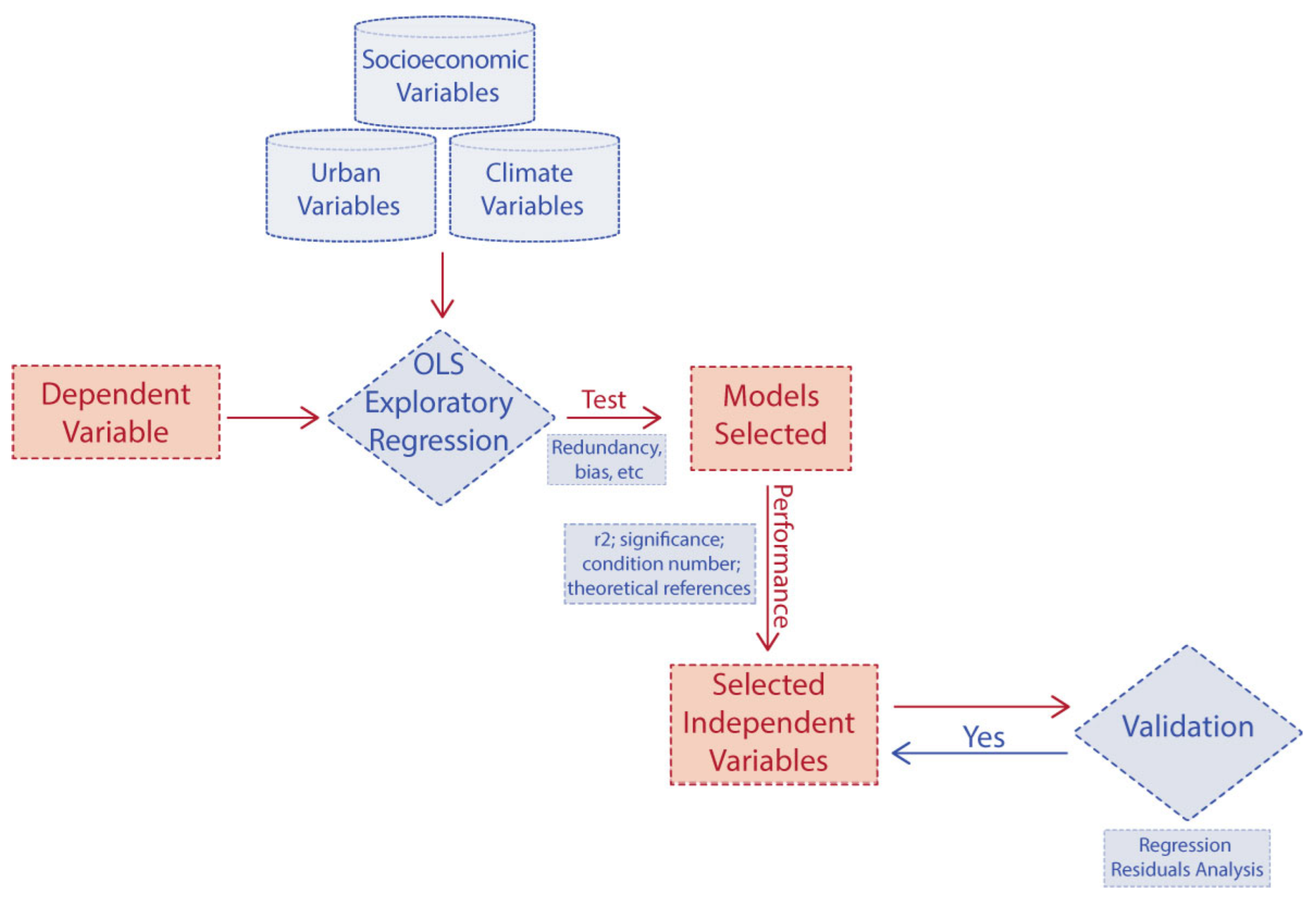
3.1. Model Selection

The survey of independent variables yielded a total combinatorial of 637 models, which is technically and conceptually not attainable, so alternatives were narrowed down by combining two techniques of exploratory statistical data analysis: (1) Multiple correlation matrix, which eliminates collinear variables (prioritizing the elimination of collinearity and thematic overlap between variables); (2) Exploratory regression to eliminate unfeasible combinations and analyze biases and significance, among other key statistics. Some of these are evident, like the annual thermal amplitude and the LST (since one is released from the other). Others are expected but not obvious (the SMTI and the percentage of professionals, the year of construction and the housing material quality indicator, mainly because they come from different databases). The criteria for defining candidate regressions and the number of regressions that meet these parameters are detailed in

Table 1. Percentage of accepted regressions according to search criteria.

Search Criteria	Cut-Off	Attempts	Successes	Percentage of Correct Answers
R2 minimum	>0.4	637	487	76.5%
p-Value	<0.05	637	379	59.5%
VIF Value	<7.50	637	637	100%
Jarque–Bera p-value	>0.10	637	11	1.7%

.

The spatial autocorrelation of the regressions is not evaluated now, assuming that it is measured in conjunction with the local multicollinearity when applying the geographically weighted regressions. Of the 11 regressions used for the GWR, only four models pass the local multicollinearity and spatial autocorrelation tests, integrating one to four independent variables (

Table 2. Description of the selected GWR models and their statistical indicators.

	Model 1	Model 2	Model 3	Model 4
Dependent variable	Inside temperature of homes in winter (year 2017)
Independent variables	NDVI	Professional percentage	Professional percentage	Professional percentage
		Land price	Land price	NDVI
			Segregation	Annual thermal amplitude
				Housing material quality
R2	0.90	0.8801	0.6841	0.8891
Average conditions	7.2	6.39	23.30	26.33
Sigma	0.2726	0.3043	0.4946	0.0859

).

Of the alternatives presented, Model 4 is used based on a multivariate explanation: (i) it has one of the highest coefficients of determination; (ii) it has the lowest sigma of all the models, which accounts for a better overall fit; and (ii) unlike Model 3, which is the multivariate model, it is easier to identify local explanations for the phenomena analyzed. In contrast, the model with only NDVI (Model 1), although it has a good mathematical performance when seeking local explanations, is not clear in all cases if it is the behavior of an underlying variable or a product of local autocorrelation. Finally, although the average conditions are higher, it is evident that better explanatory power is obtained in a geographically weighted regression model with more variables, even with an average of 26.33. The variables chosen are related to the energy poverty phenomenon and are consistent with the spatial modelling. The materiality of the housing accounts for the insulation problems in both summer and winter. Vegetation performs as an attenuator of extreme temperature. However, its distribution is also related to the sociodemographic composition, while the annual thermal amplitude is a proxy variable that directly affects the variations of the dependent variable. It is relevant to note that the SMTI has not been considered in any model since it presents collinearity with other variables (housing material quality index and percentage of professionals). This situation may infuse noise into the model through local multicollinearity. Therefore, including it as an explanatory variable in the regression model is not helpful in this case, despite the lack of this variable in providing substantial evidence. Nevertheless, in replacement for this lack, the percentage of professionals was used, measured by the years of schooling, which is also the primary constituent variable of the SMTI, having an average weight of around 78% in a performed principal component analysis. By analyzing the results of the final model, some clear spatial patterns can be established, as well as practical considerations concerning the statistics generally produced by the model.

3.2. Interpretation: Spatial Patterns of Energy Poverty in the Metropolitan Area of Santiago de Chile

The first important aspect is that the model has a low sigma, so the high residual standard deviations are referred to in this case as discrepancies of (+) (−) 1.4 °C. There is some observable spatial autocorrelation which does not invalidate the model. However, it would be advisable to have a sample with a higher level of the spatial grain of the dependent variable, which would allow more in-depth observations, even more, detailed than those that will be defined below, according to the different urban areas:

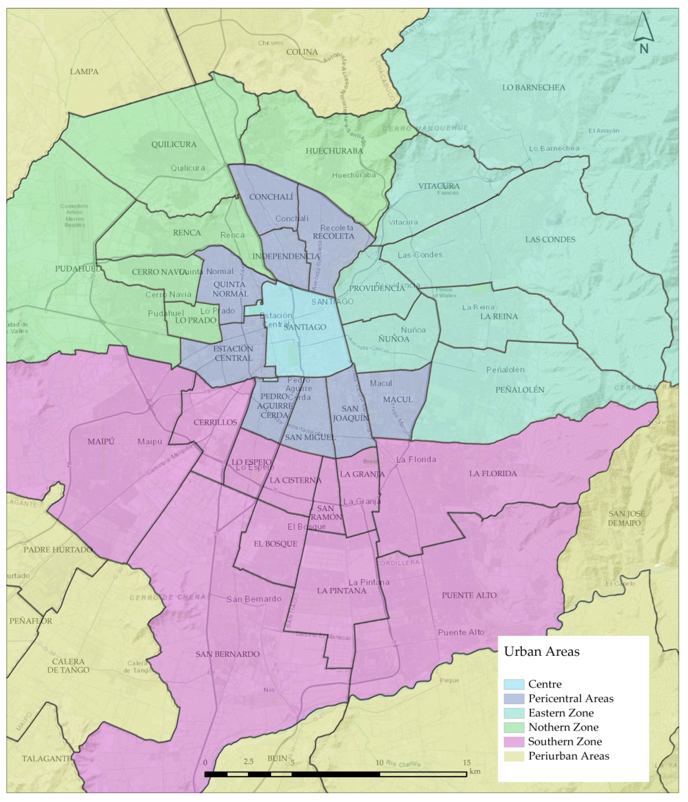
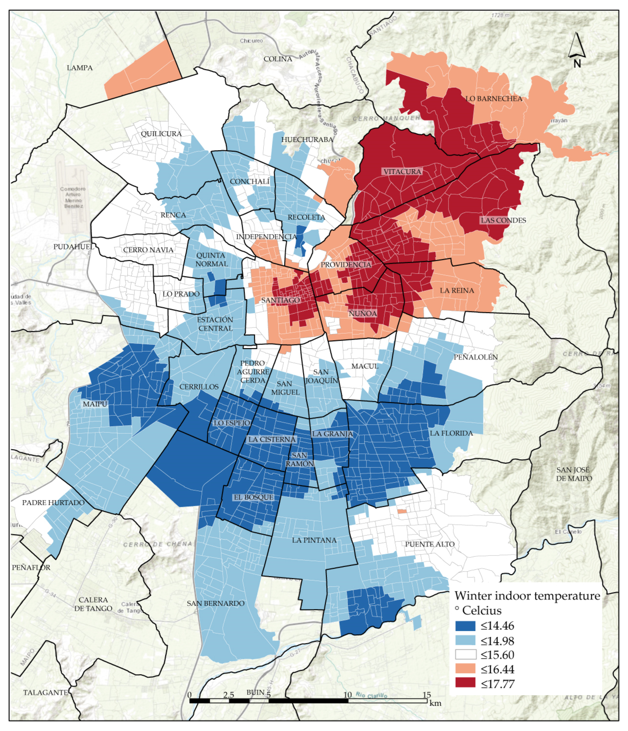
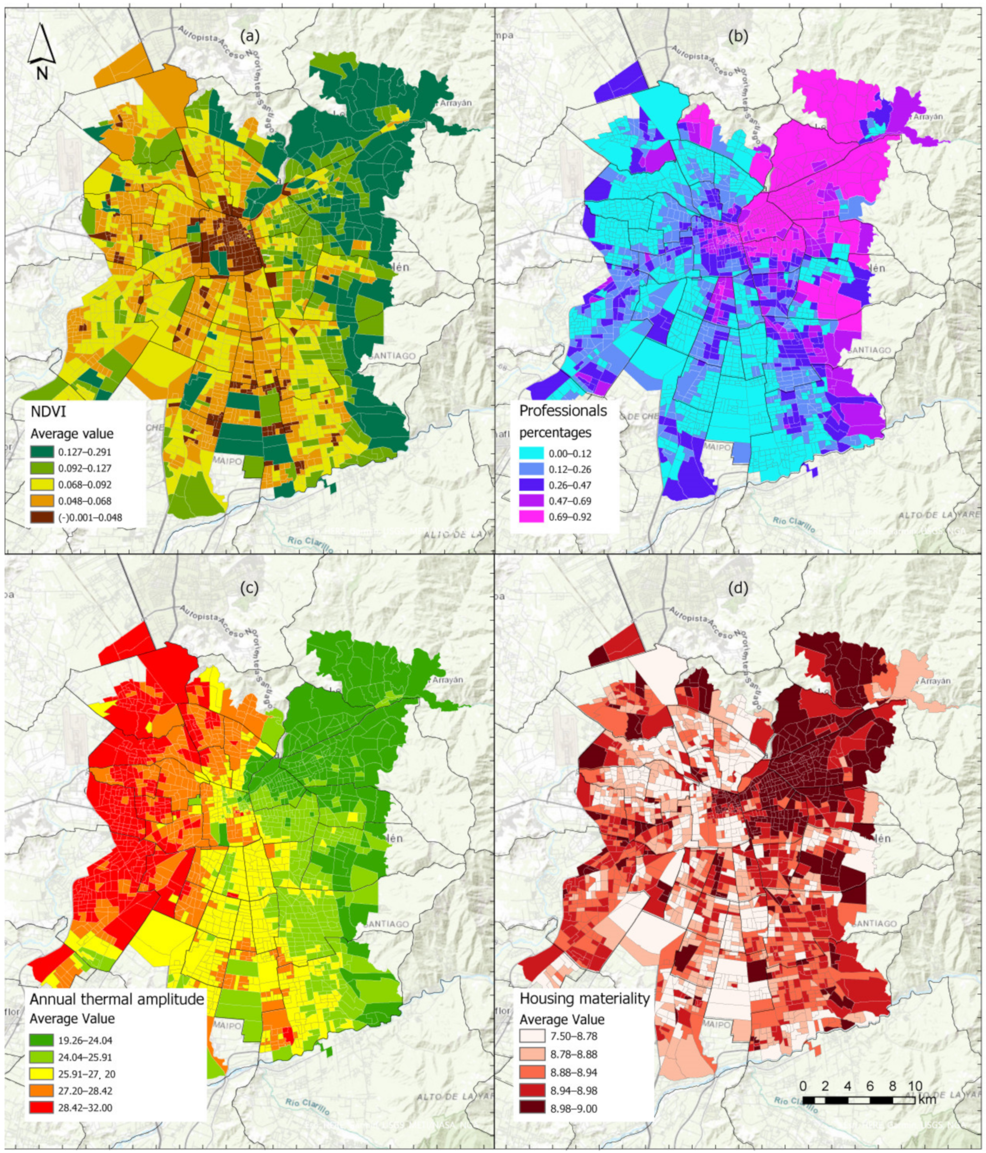
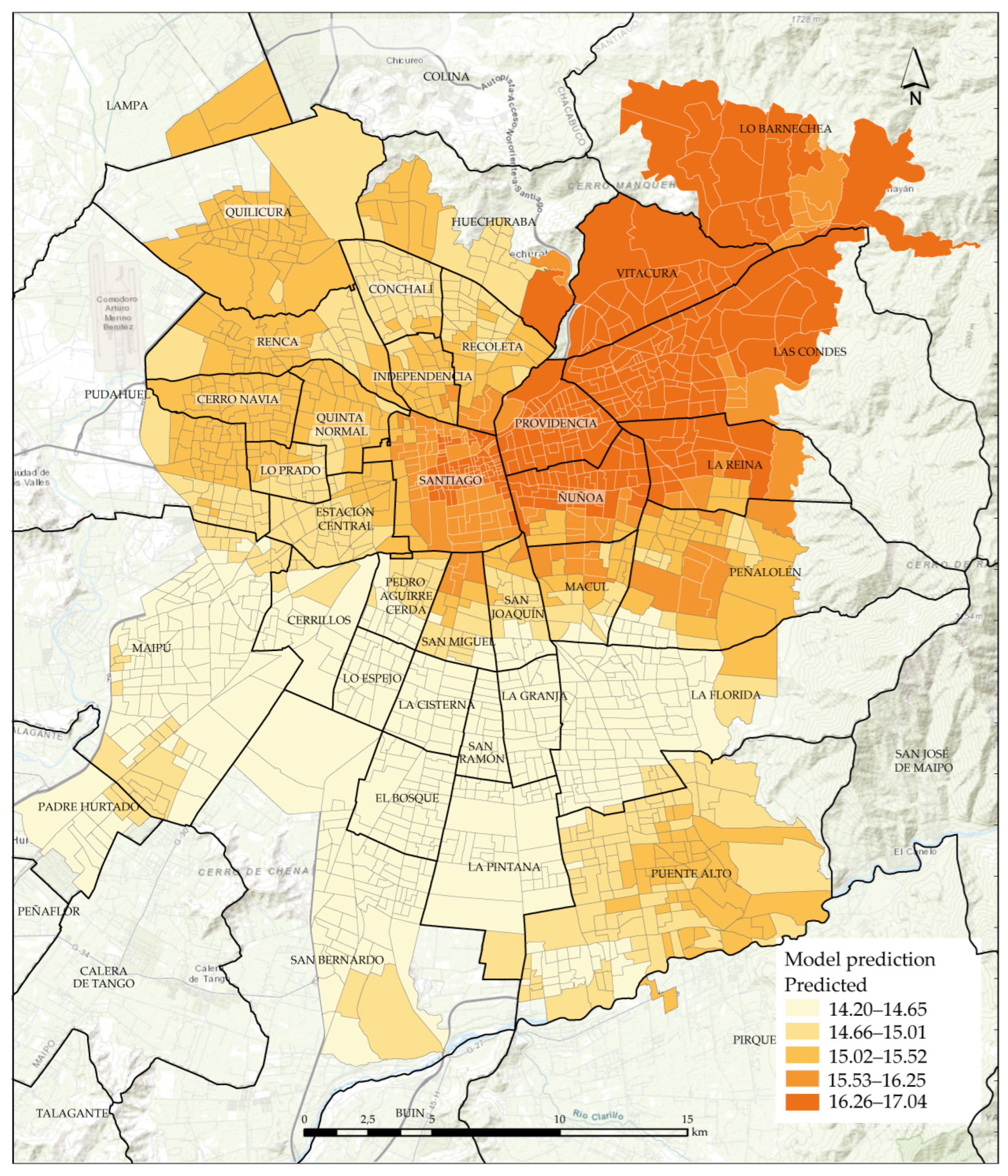
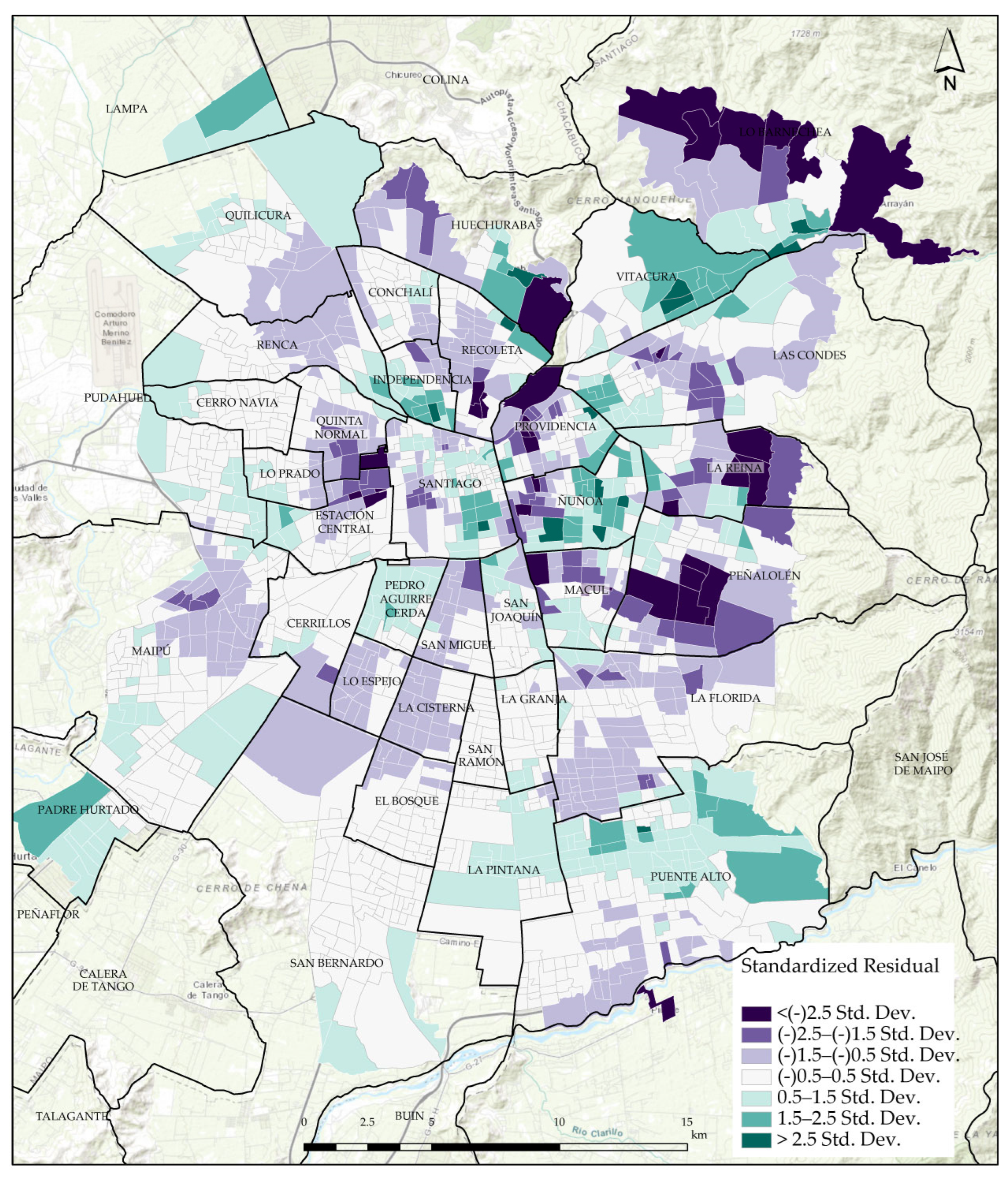
• Eastern Area: in Santiago’s metropolitan area, the higher income sectors are concentrated in “a sort of triangle that has one of its vertices in the commune of Santiago and then stretches towards the northeast, covering a good part of the mountain slopes” [79]. The so-called “high-income cone” [80] has been characterized by processes of spatial self-segregation [81]. In the model, it is expressed with a defined pattern to the dependent variable. Here, there are high inside temperatures transversal to the communes that compose it (Ñuñoa, La Reina, Providencia, Las Condes, Vitacura, and Lo Barnechea). Specifically, the highest values occur in the eastern boundary of the commune of Santiago, the northeastern zone of Ñuñoa, west of La Reina, the vast majority of Providencia and Las Condes, the western sector of Lo Barnechea, and uniformly for the entire commune of Vitacura (Figure 3). The general pattern is reinforced with the four variables of the model. Still, specifically for the highest temperatures, the variables that operate at the local level are the material of the home together with the annual thermal amplitude. This situation is evident when observing the agglomeration of high-temperature sectors in Santiago, which also coincides with the higher percentages of professionals and a greater vegetation cover and green areas expressed in the NDVI (Figure 5). In terms of standardized residuals, the most overestimated place is the foothills of this high-income cone (expressed through lower temperatures in winter), where the geographical factor prevails. The opposite case occurs in some vulnerable enclaves of these communes where the percentage of professionals decreases as well as the material quality of the homes. Still, the other environmental variables remain constant, causing the model to underestimate the observations.
• Pericentral area: in the communes surrounding the center of the metropolitan area of Santiago (Recoleta, Independencia, Quinta Normal, Estación Central and Pedro Aguirre Cerda), there is a pattern of lower temperatures inside the homes in winter compared to the center of the consolidated urban area (Figure 3). Two independent variables mainly explain this: (1) the material quality of the housing is generally precarious, associated in many cases with self-construction processes. This is also reinforced with the second variable that, in this case, corresponds to the almost zero presence of vegetation detected by the (2) NDVI indicator, a situation that is not only expressed as access to public green areas but also more strongly as lack of public trees and private vegetation (inside the home.) The exceptions for this spatial pattern are expressed by the values overestimated by the model (higher temperatures) for part of the commune of San Miguel (neighborhood known as the Llano Subercaseaux) given its higher socioeconomic nature and the better-quality housing material. This is because they are homes built with recent regulations, an urban renewal sector in the verticalization process. The second milestone is the area around the Quinta Normal urban park—a situation associated in this case with the presence of vegetation—which should help mitigate temperatures, which does not occur as the model predicted.
• Northern area: the pattern of inside temperatures of the homes is slightly higher than expected, given the characteristics of the socioeconomic vulnerability of the area, combined with a low presence of vegetation and low material quality indices of the home (Figure 5). This is mainly explained by the behavior of the thermal amplitude, which determines the model in this extensive area of the metropolitan area of Santiago (communes of Lo Prado, Cerro Navia, Renca, and Quilicura). The values of thermal amplitude are the highest, which translates into higher maximum temperatures in summer. However, slightly higher minimum temperatures are also observed in winter, which defines an extensive pattern of inside temperatures in homes somewhat higher than the rest of the peripheral areas (but in this case, not due to housing material).
• Southern area: In terms of the dependent variable, the lowest temperature values inside the homes during the winter occur in the communes of Maipú, Lo Espejo, San Ramón, La Granja, La Florida, San Bernardo, La Pintana, and Puente Alto (Figure 3). In this case, the lowest values of the four independent variables are combined to justify the values observed and estimated by the geographically weighted regression model, with extreme cases in particularly vulnerable areas, such as the Bajo de Mena sector, south of the commune of Puente Alto.

3.3. Validation of the Model

In general, terms, the model applies very well given the equilibrium provided by having a multivariate explanatory function (Figure 6). At the same time, the condition number, which accounts for local multicollinearity, is below the limit of 30 in all the census tract units, which shows the feasibility of the GWR model. This indicator is especially significant considering that the dependent variable (indoor temperature of the houses) comes from an interpolation. However, the standard deviation of the standardized residuals accounts for better fits in some map locations (greater than 2.5 standard deviations correspond to estimated differences versus the observed of only 1.4 °C) (Figure 7). With this, in terms of methodological aspects, it is possible to affirm that local multicollinearity can be increased slightly—consistently within the acceptable range of the GWR model—to obtain stronger arguments for analyzing the results.

In addition to this analysis, it is possible to observe the non-correlation between the standardized residuals and the predicted values, which is essential to give reliability to the model (Figure 8). In this sense, it is evident that a trend does not exist between the values obtained from the model and the model errors.

Additionally, traditional testing methods for the GWR model indicate the need to examine the clustering level of the (unstandardized) residuals. It is assumed that when there is a high Moran index, we have some unknown variables that should be explored and considered for the model. For the Moran Index, a matrix of spatial weights of K neighbors was used, the same as the regression neighborhood, to maintain the consistency of the method (Figure 9). The result is indeed clustered but with a low Moran Index value, indicating that the problems of the model are minor.

4. Discussion

With the results presented, several lessons can be extracted that indicate, on the one hand, the ability of the model to link a set of socioeconomic, urban, and climatic variables, allowing an interpretation based on energy poverty; on the other hand, as a model of these characteristics, it can propose a spatial analysis of urban and climate implications, contributing evidence to decision-making for public policy.

Strictly speaking, from the specificity of the GWR model, one can argue the need for more precise global variables. An example is housing material. A specific definition of the thermal envelope can be inferred but does not directly constitute this factor, presenting the percentage of substandard housing and not a direct metric of this factor. Still, this does not add heterogeneity to the GWR model but would allow it to be more conclusive with the model. Public agencies must be able to register the technical definition of the different elements of the housing envelope (e.g., walls, windows, and roofs) to improve these indicators.

Similarly, exploring beyond NDVI could provide more detail about how vegetation types directly affect mitigating extreme temperatures. On the other hand, from the sphere of spatial quality, it would be recommended to have a dependent variable with a better sampling frame (statistical representativeness) and given the significant spatial autocorrelation inherent in the variable, it seems wise to explore alternatives based on spatialized sampling [82,83,84]. This implies generating a plausible explanatory scheme associated with energy poverty and urging census and sample instruments to include this information to better position this issue as an evaluable public policy through spatial indicators sensitive to temporal monitoring. In this regard, it is essential to mention the possibility of adding a territorial specificity factor, as indicated by Rodríguez-Iglesias and López [85] to reveal the urban particularities that may be significant when developing the indicator or its standards, given the climatic and geographical diversity of the national territory.

On the other hand, one of the study’s main findings is identifying a housing quality pattern that acts as a proxy for vulnerability to energy poverty, repeating the distribution pattern of the different socioeconomic sectors. This point is relevant in the context of the discussion on urban segregation [62], where the conditions of liberating the land and housing market exacerbate energy poverty by allocating homes with a low technical standard in locations with low urban attributes that allow—for example—to mitigate thermal fluctuations through the incorporation of green areas. On the other hand, the role of professional heads of households in explaining the relationships of energy poverty allows a rough approximation; however, it is critical to have block-level data on average household income to improve these data. Although the educational level of heads of household and occupational groups is a method widely validated by the literature to generate a proxy of the socioeconomic status of households, the high degree of inequality and how it is distributed in Chile may cause this factor to lose precision. Improving the socioeconomic statistical sampling of grain is key to effectively identifying these patterns in cities. This finding is aligned with the observations provided by Munro and Samarakoon, and Bouzarovski. They indicated how the reliance on free-market urban economics triggers inequalities represented in energy poverty and undermines the efforts of planning solutions by the State [25,27]. The role of free-market urban economics in energy poverty is a common discussion in the revised literature. It seems like the thesis of Kocack and Baglitas on how that income inequality reproduces energy poverty [20] implies that resolving these issues will demand a more interdisciplinary approach to the case, ranging from housing policies to financial regulations, including macroeconomic factors as indicated by Primc et al. [19].

Croce and Tondini pointed out the importance of improving and exploring ways to measure city energy poverty [24]. This article provides an approach which was not previously applied to the case of Chile, with relevant findings as pointed out above. In this sense, a diagram summarizes the interactions and conditions that would improve the methodological quality of the model to better understand the housing situation under conditions of energy poverty (Figure 10). This, from a multidimensional logic that articulates socioeconomic, urban, and climatic variables—as this article questioned at the beginning—and that spatial analysis can explain energy poverty from three types of vulnerability: socio-spatial, territorial, and territorial socioenvironmental.

As Hidalgo argues, the dominance of the free market in urban development, coupled with the ‘State’s” inability to generate significant advances in spatial justice, is a sure path to the precariopolis [20]. This precarious, dystopian, and unjust city is no stranger to the reality of different neighborhoods in the Santiago Metropolitan Area when analyzed from the perspective of energy poverty. The articulation between the housing market and territorial planning instruments needs to coordinate an approach that reduces the socio-spatial effects of their contradictions.

5. Conclusions

The study results have allowed a methodology to develop maps of energy poverty, taking the metropolitan area of Santiago de Chile as a specific case. The use of the GWR analysis technique is innovative and has generated findings that can contribute to improving territorial planning instruments for the Santiago Metropolitan Area. As a spatial regression model, it presents methodological limitations, which were approached through variable control and specific statistical analysis. In addition, applying this analysis technique opens a space for discussion on the cross-cutting relationships between energy poverty and other inequalities represented in the urban space of Santiago. One of the main inequalities is the quality of the data, for which it is suggested to move towards a national census that accurately measures the quality of construction. In Chile, a new population census will be implemented in 2024, which presents an excellent opportunity to implement this measurement, considering the urgency of the energy poverty problem highlighted in this article.

The levels of socio-spatial inequality of this metropolis offer ad hoc conditions to measure the precision of this type of analysis, where high residential segregation and free-market urban development allow the application of a ceteris paribus (in the context of urban econometric studies). In this scenario, the understanding of energy poverty as an unequally distributed factor in the city is deepened, expressed through the interaction of three types of vulnerability: socio-spatial, territorial, and socio-environmental. Alternative findings inform decision-makers about the importance of generating comprehensive urban policies on a more precise scale than the level of communes. Added to this is the critical observation of official data, which are currently insufficient to generate diagnoses that effectively improve resource targeting strategies. Applying energy poverty questions in the next census or the national socioeconomic survey (CASEN) in 2024 is critical to advance a better diagnosis of the problem.

The findings incorporate a new interpretive matrix into the already complex reproduction of the precariópolis in Santiago de Chile, as Hidalgo et al. [20] observed. The different clusters in the territory indicate that energy poverty proliferates in sectors where social housing has been produced or urban renewal via private condominiums has shaped these spaces. Historically the construction of social housing in Chile has been based on low-cost solutions using the minimum building standards, which has undermined the advance toward social spaces where energy poverty is reduced. Although new regulations aim to tackle this problem, free-market urban production is still ruling the urban development of Chilean cities. Reversing this trend requires stricter housing policy regulations and making residential technical requirements in Chile adapt to the urgent needs of the current climate emergency. These requirements may assume a more aggressive retroactive role than they have had thus far, providing more significant resources for improving existing homes. The main topics to address in these regulations are the thermal envelope, passive climatic techniques, and equal construction standards independent of the household’s average income. The question to advance in these matters is how to accomplish it without triggering a boost in housing prices. However, evidence indicates that better construction standards are not the leading cause of increasing prices in Chile [62]. A passive strategy from the State is no longer socially and environmentally sustainable. A necessary shift is urgent.

As has been indicated, the concern about energy poverty is urgent, even more so considering that the household budget in Chile is highly pressurized by the high cost of living, which is underrepresented in the official instruments for measuring inflation. This mechanism also ignored spatial diversity [86]. One of the main contributions of this article is to identify the socio-spatial distribution of energy poverty, providing an exploratory model whose application in other cities can estimate the impact of socioeconomic, urban, and climatic variables at the territorial scale on the performance and comfort of cities and homes on a domestic scale, thus fulfilling its initial objective. Further research may be undertaken by sampling the different areas of the city identified as conducting qualitative research based on fieldwork to collect primary data and then testing the results of this analysis, focusing on a broader scale. In addition, the results must be presented to decision-makers considering the relevance of the matters. Researchers must also communicate the results to a broader audience and ensure that the Housing Ministry and the Parliament are aware of the importance of regulating housing quality to reduce energy poverty.

References

1. Kerr, N.; Gillard, R.; Middlemiss, L. Politics, Problematisation, and Policy: A Comparative Analysis of Energy Poverty in England, Ireland and France. Energy Build. 2019, 194, 191–200. [Google Scholar] [CrossRef]
2. Primc, K.; Slabe-Erker, R.; Majcen, B. Constructing Energy Poverty Profiles for an Effective Energy Policy. Energy Policy 2019, 128, 727–734. [Google Scholar] [CrossRef]
3. Walker, G.; Day, R. Fuel Poverty as Injustice: Integrating Distribution, Recognition and Procedure in the Struggle for Affordable Warmth. Energy Policy 2012, 49, 69–75. [Google Scholar] [CrossRef]
4. Hills, J. Getting the Measure of Fuel Poverty: Final Report of the Fuel Poverty Review. CASE Report 72; Centre for Analysis of Social Exclusion, The London School of Economics and Political Science: London, UK, 2012. [Google Scholar]
5. Boardman, B. Fuel Poverty: From Cold Homes to Affordable Warmth; Wiley and Sons: London, UK, 1991. [Google Scholar]
6. Liddell, C. Fuel Poverty Comes of Age: Commemorating 21 Years of Research and Policy. Energy Policy 2012, 49, 2–5. [Google Scholar] [CrossRef]
7. Rademaekers, K.; Yearwood, J.; Ferreira, A.; Pye, S.; Hamilton, I.; Agnolucci, P.; Grover, D.; Karásek, J.; Animisova, N. Selecting Indicators to Measure Energy Poverty; Trinomics, B.V.: Rotterdam, The Netherlands, 2016. [Google Scholar]
8. Moore, R. Definitions of Fuel Poverty: Implications for Policy. Energy Policy 2012, 49, 19–26. [Google Scholar] [CrossRef]
9. Boardman, B. Fixing Fuel Poverty: Challenges and Solutions; Earthscan: London, UK, 2010. [Google Scholar]
10. González-Eguino, M. Energy Poverty: An Overview. Renew. Sustain. Energy Rev. 2015, 47, 377–385. [Google Scholar] [CrossRef]
11. Calvo, R.; Amigo, C.; Billi, M.; Cortés, A.; Mendoza, P.; Tapia, R.; Urquieta, M.A.; Urquiza, A. Acceso Equitativo a Energía de Calidad en Chile: Hacia un Indicador Territorializado y Tridimensional de Pobreza Energética; Red de Pobreza Energética: Santiago, Chile, 2019; ISBN 978-956-398-826-0. [Google Scholar]
12. United Nations. Transforming Our World: The 2030 Agenda for Sustainable Development; United Nations: New York, NY, USA, 2015. [Google Scholar]
13. Ministerio de Energía. Transición Energética de Chile. Política Energética Nacional. Actualización 2022; Ministerio de Energía: Santiago, Chile, 2022.
14. Bridge, B.A.; Adhikari, D.; Fontenla, M. Electricity, Income, and Quality of Life. Soc. Sci. J. 2016, 53, 33–39. [Google Scholar] [CrossRef]
15. Vilches, A.; Barrios Padura, Á.; Molina Huelva, M. Retrofitting of Homes for People in Fuel Poverty: Approach Based on Household Thermal Comfort. Energy Policy 2017, 100, 283–291. [Google Scholar] [CrossRef]
16. Igawa, M.; Managi, S. Energy Poverty and Income Inequality: An Economic Analysis of 37 Countries. Appl. Energy 2022, 306, 118076. [Google Scholar] [CrossRef]
17. Bouzarovski, S. Energy Poverty in the European Union: Landscapes of Vulnerability. Wiley Interdiscip. Rev. Energy Environ. 2014, 3, 276–289. [Google Scholar] [CrossRef]
18. Buzar, S. Energy Poverty in Eastern Europe: Hidden Geographies of Deprivation; Routledge: Boca Raton, FL, USA, 2007. [Google Scholar]
19. Primc, K.; Slabe-Erker, R.; Majcen, B. Energy Poverty: A Macrolevel Perspective. Sustain. Dev. 2019, 27, 982–989. [Google Scholar] [CrossRef]
20. Hidalgo, R.; Borsdorf, A.; Zunino, H.M.; Álvarez, L. Tipologías de Expansión Metropolitana En Santiago de Chile: Precariópolis Estatal y Privatópolis Inmobiliaria. Scr. Nova Rev. Electrónica Geogr. Cienc. Soc. 2008, 12, 113. [Google Scholar]
21. Kocak, E.; Baglitas, H.H. The Path to Sustainable Municipal Solid Waste Management: Do Human Development, Energy Efficiency, and Income Inequality Matter? Sustain. Dev. 2022, 1–16. [Google Scholar] [CrossRef]
22. Guzmán-Rosas, S.C. Ethnicity as a Social Determinant of Energy Poverty: The Case of Mexican Indigenous Population. Local Environ. 2022, 27, 1075–1101. [Google Scholar] [CrossRef]
23. Caprotti, F.; de Groot, J.; Bobbins, K.; Mathebula, N.; Butler, C.; Moorlach, M.; Schloemann, H.; Densmore, A.; Finlay, K. Rethinking the Off-Grid City. Urban Geogr. 2022, 1–14. [Google Scholar] [CrossRef]
24. Croce, S.; Tondini, S. Fixed and Mobile Low-Cost Sensing Approaches for Microclimate Monitoring in Urban Areas: A Preliminary Study in the City of Bolzano (Italy). Smart Cities 2022, 5, 54–70. [Google Scholar] [CrossRef]
25. Bouzarovski, S. Just Transitions: A Political Ecology Critique. Antipode 2022, 54, 1003–1020. [Google Scholar] [CrossRef]
26. Alabi, O.; Abubakar, A.; Werkmeister, A.; Sule, S.D. Keeping the Lights On or Off: Tracking the Progress of Access to Electricity for Sustainable Development in Nigeria. GeoJournal 2022, 1–24. [Google Scholar] [CrossRef]
27. Munro, P.G.; Samarakoon, S. Off-Grid Electrical Urbanism: Emerging Solar Energy Geographies in Ordinary Cities. J. Urban Technol. 2022, 1–24. [Google Scholar] [CrossRef]
28. Chipango, E.F. Political Ecologies of Energy Poverty in Zimbabwe. GeoJournal 2022, 1–15. [Google Scholar] [CrossRef]
29. Bîrsănuc, E.-M. Mapping Gendered Vulnerability to Energy Poverty in Romania. Appl. Spat. Anal. Policy 2022, 1–20. [Google Scholar] [CrossRef]
30. Bouzarovski, S.; Simcock, N. Spatializing Energy Justice. Energy Policy 2017, 107, 640–648. [Google Scholar] [CrossRef]
31. März, S. Assessing the Fuel Poverty Vulnerability of Urban Neighbourhoods Using a Spatial Multi-Criteria Decision Analysis for the German City of Oberhausen. Renew. Sustain. Energy Rev. 2018, 82, 1701–1711. [Google Scholar] [CrossRef]
32. Robinson, C.; Lindley, S.; Bouzarovski, S. The Spatially Varying Components of Vulnerability to Energy Poverty. Ann. Am. Assoc. Geogr. 2019, 109, 1188–1207. [Google Scholar] [CrossRef]
33. Reames, T.G. Targeting Energy Justice: Exploring Spatial, Racial/Ethnic and Socioeconomic Disparities in Urban Residential Heating Energy Efficiency. Energy Policy 2016, 97, 549–558. [Google Scholar] [CrossRef]
34. Scarpellini, S.; Sanz Hernández, M.A.; Moneva, J.M.; Portillo-Tarragona, P.; López Rodríguez, M.E. Measurement of Spatial Socioeconomic Impact of Energy Poverty. Energy Policy 2019, 124, 320–331. [Google Scholar] [CrossRef]
35. López-Bueno, J.A.; Díaz, J.; Sánchez-Guevara, C.; Sánchez-Martínez, G.; Franco, M.; Gullón, P.; Núñez Peiró, M.; Valero, I.; Linares, C. The Impact of Heat Waves on Daily Mortality in Districts in Madrid: The Effect of Sociodemographic Factors. Environ. Res. 2020, 190, 109993. [Google Scholar] [CrossRef]
36. Martín-Consuegra, F.; Hernández-Aja, A.; Oteiza, I.; Alonso, C. Distribución de La Pobreza Energética En La Ciudad de Madrid (España). EURE-Rev. Estud. Urbano Reg. 2019, 45, 133–152. [Google Scholar] [CrossRef]
37. Sanusi, Y.A.; Owoyele, G.S. Energy Poverty and Its Spatial Differences in Nigeria: Reversing the Trend. Energy Procedia 2016, 93, 53–60. [Google Scholar] [CrossRef]
38. Gupta, S.; Gupta, E.; Sarangi, G.K. Household Energy Poverty Index for India: An Analysis of Inter-State Differences. Energy Policy 2020, 144, 111592. [Google Scholar] [CrossRef]
39. Marchand, R.; Genovese, A.; Koh, S.C.L.; Brennan, A. Examining the Relationship between Energy Poverty and Measures of Deprivation. Energy Policy 2019, 130, 206–217. [Google Scholar] [CrossRef]
40. Moore, D.; Webb, A.L. Evaluating Energy Burden at the Urban Scale: A Spatial Regression Approach in Cincinnati, Ohio. Energy Policy 2022, 160, 112651. [Google Scholar] [CrossRef]
41. García-Ochoa, R.; Graizbord, B. Privation of Energy Services in Mexican Households: An Alternative Measure of Energy Poverty. Energy Res. Soc. Sci. 2016, 18, 36–49. [Google Scholar] [CrossRef]
42. Pérez-Fargallo, A.; Bienvenido-Huertas, D.; Rubio-Bellido, C.; Trebilcock, M. Energy Poverty Risk Mapping Methodology Considering the User’s Thermal Adaptability: The Case of Chile. Energy Sustain. Dev. 2020, 58, 63–77. [Google Scholar] [CrossRef]
43. Chen, H.-C.; Han, Q.; de Vries, B. Modeling the Spatial Relation between Urban Morphology, Land Surface Temperature and Urban Energy Demand. Sustain. Cities Soc. 2020, 60, 102246. [Google Scholar] [CrossRef]
44. Meng, Y.; Xing, H.; Yuan, Y.; Wong, M.S.; Fan, K. Sensing Urban Poverty: From the Perspective of Human Perception-Based Greenery and Open-Space Landscapes. Comput. Environ. Urban Syst. 2020, 84, 101544. [Google Scholar] [CrossRef]
45. Shaker, R.R.; Altman, Y.; Deng, C.; Vaz, E.; Forsythe, K.W. Investigating Urban Heat Island through Spatial Analysis of New York City Streetscapes. J. Clean. Prod. 2019, 233, 972–992. [Google Scholar] [CrossRef]
46. Tu, M.; Liu, Z.; He, C.; Fang, Z.; Lu, W. The Relationships between Urban Landscape Patterns and Fine Particulate Pollution in China: A Multiscale Investigation Using a Geographically Weighted Regression Model. J. Clean. Prod. 2019, 237, 117744. [Google Scholar] [CrossRef]
47. Robinson, C.; Bouzarovski, S.; Lindley, S. Underrepresenting Neighbourhood Vulnerabilities? The Measurement of Fuel Poverty in England. Environ. Plan. A Econ. Space 2018, 50, 1109–1127. [Google Scholar] [CrossRef]
48. O’Sullivan, D. Geographically Weighted Regression: The Analysis of Spatially Varying Relationships (Review). Geogr. Anal. 2010, 35, 272–275. [Google Scholar] [CrossRef]
49. Páez, A.; Farber, S.; Wheeler, D. A Simulation-Based Study of Geographically Weighted Regression as a Method for Investigating Spatially Varying Relationships. Environ. Plan. A Econ. Space 2011, 43, 2992–3010. [Google Scholar] [CrossRef]
50. Griffith, D.A. A Linear Regression Solution to the Spatial Autocorrelation Problem. J. Geogr. Syst. 2000, 2, 141–156. [Google Scholar] [CrossRef]
51. Sánchez-Peña, L.L. Alcances y Límites de Los Métodos de Análisis Espacial Para El Estudio de La Pobreza Urbana. Pap. Población 2012, 18, 147–180. [Google Scholar]
52. INE; MINVU. Metodología Para Medir el Crecimiento Urbano de Las Ciudades de Chile; Ministerio de Vivienda y Urbanismo: Santiago, Chile, 2017.
53. Vergara-Perucich, J.F. Aplicaciones de La Teoría Implosión/Explosión: Relación Entre La Región Metropolitana de Santiago de Chile y Los Territorios Productivos Regionales. EURE-Rev. Estud. Urbano Reg. 2018, 44, 71–90. [Google Scholar] [CrossRef]
54. Celedon Forster, A. Operación Piloto: Santiago En Tres Actos. Revista 180 2019, 43, 1–12. [Google Scholar] [CrossRef]
55. Gross, P. Santiago de Chile (1925–1990): Planificación Urbana y Modelos Políticos. EURE-Rev. Estud. Urbano Reg. 1991, 17, 27–52. [Google Scholar]
56. Vergara-Perucich, F.; Boano, C. The Big Bang of Neoliberal Urbanism: The Gigantomachy of Santiago’s Urban Development. Environ. Plan. C Politics Space 2021, 39, 184–203. [Google Scholar] [CrossRef]
57. Garreton, M. City Profile: Actually Existing Neoliberalism in Greater Santiago. Cities 2017, 65, 32–50. [Google Scholar] [CrossRef]
58. Donoso, F.; Sabatini, F. Santiago: Empresa Inmobiliaria Compra Terrenos. EURE-Rev. Estud. Urbano Reg. 1980, 7, 25–51. [Google Scholar]
59. Trivelli, P. Accesibilidad al Suelo Urbano y La Vivienda Por Parte de Los Sectores de Menos Ingresos En América Latina. EURE-Rev. Estud. Urbano Reg. 1982, 9, 7–32. [Google Scholar]
60. Sabatini, F.; Brain, I. La Segregación, Los Guetos y La Integración Social Urbana: Mitos y Claves. EURE-Rev. Estud. Urbano Reg. 2008, 34, 5–26. [Google Scholar] [CrossRef]
61. Hidalgo, R. ¿Se Acabo El Suelo En La Gran Ciudad? Las Nuevas Periferias Metropolitanas de La Vivienda Social En Santiago de Chile. EURE-Rev. Estud. Urbano Reg. 2007, 33, 57–75. [Google Scholar] [CrossRef]
62. Encinas, F.; Aguirre, C.; Vergara-Perucich, F.; Tironi, M.; Truffello, R.; Freed, C.; Hidalgo, R. Disciplinary Inflections: Contesting Three Concepts for the Construction of the Post-Neoliberal City. ARQ 2021, 107, 46–57. [Google Scholar] [CrossRef]
63. Vergara-Perucich, F.; Aguirre, C.; Encinas, F.; Truffello, R.; Ladrón de Guevara, F. Contribución a la Economía Política de la Vivienda en Chile; RiL Editores: Santiago, Chile, 2020. [Google Scholar]
64. Sarricolea Espinoza, P.; Martín-Vide, J. El Estudio de La Isla de Calor Urbana de Superficie Del Área Metropolitana de Santiago de Chile Con Imágenes Terra-MODIS y Análisis de Componentes Principales. Rev. Geogr. Norte Gd. 2014, 123–141. [Google Scholar] [CrossRef]
65. Montaner-Fernández, D.; Morales-Salinas, L.; Rodriguez, J.S.; Cárdenas-Jirón, L.; Huete, A.; Fuentes-Jaque, G.; Pérez-Martínez, W.; Cabezas, J. Spatio-Temporal Variation of the Urban Heat Island in Santiago, Chile during Summers 2005–2017. Remote Sens. 2020, 12, 3345. [Google Scholar] [CrossRef]
66. Romero, H.; Vásquez, A.; Fuentes, C.; Salgado, M.; Schmidt, A.; Banzhaf, E. Assessing Urban Environmental Segregation (UES). The Case of Santiago de Chile. Ecol. Indic. 2012, 23, 76–87. [Google Scholar] [CrossRef]
67. Calvo, R.; Amigo, C.; Billi, M.; Fleischmann, M.; Urquiza, A. Vulnerabilidad Energética Territorial: Desigualdad Mas Allá del Hogar; Red de Pobreza Energética: Santiago, Chile, 2020; ISBN 978-956-402-385-4. [Google Scholar]
68. MINVU RENAM-Red Nacional de Monitoreo. Available online: https://renam.cl (accessed on 20 July 2022).
69. González, K.; Amigo, C.; Calvo, R.; Oyarzún, T.; San Martín, M.; Urquiza, A.; Álvarez, M.; Hidalgo, F.; Muñoz, F.; Tapia, T.; et al. Una Mirada Multidimensional a la Pobreza Energética en Chile; Red de Pobreza Energética and Generadoras de Chile: Santiago, Chile, 2022. [Google Scholar]
70. Becerra, M.; Jerez, A.; Valenzuela, M.; Garcés, H.O.; Demarco, R. Life Quality Disparity: Analysis of Indoor Comfort Gaps for Chilean Households. Energy Policy 2018, 121, 190–201. [Google Scholar] [CrossRef]
71. Castaño-Rosa, R.; Solís-Guzmán, J.; Rubio-Bellido, C.; Marrero, M. Towards a Multiple-Indicator Approach to Energy Poverty in the European Union: A Review. Energy Build. 2019, 193, 36–48. [Google Scholar] [CrossRef]
72. Urquiza, A.; Amigo, C.; Billi, M.; Leal, T. Pobreza Energética en Chile: ¿Un Problema Invisible? Análisis de Fuentes Secundarias Disponibles de Alcance Nacional; Red de Pobreza Energética, Universidad de Chile: Santiago, Chile, 2017. [Google Scholar]
73. OCUC. Observatorio de Ciudades UC. Centro de Investigación Urbano-Territorial. Available online: https://observatoriodeciudades.com (accessed on 20 July 2022).
74. CENSO. 2017 Microdatos Censo. 2017. Available online: http://www.censo2017.cl/microdatos/ (accessed on 20 July 2022).
75. USGS. Landsat 8. Available online: https://earthexplorer.usgs.gov (accessed on 20 July 2022).
76. Encinas, F.; Truffello, R.; Aguirre, C.; Hidalgo, R. Speculation, Land Rent, and the Neoliberal City. Or Why Free Market Is Not Enough. ARQ 2019, 120–133. [Google Scholar] [CrossRef]
77. OIT. Clasificación Internacional Uniforme de Ocupaciones; International Labour Office: Geneva, Switzerland, 2008. [Google Scholar]
78. Parisi, D.; Lichter, D.T.; Taquino, M.C. Multi-Scale Residential Segregation: Black Exceptionalism and America’s Changing Color Line. Soc. Forces 2011, 89, 829–852. [Google Scholar] [CrossRef]
79. De Mattos, C.A. Mercado Metropolitano de Trabajo y Desigualdades Sociales En El Gran Santiago: ¿Una Ciudad Dual? EURE-Rev. Estud. Urbano Reg. 2002, 28, 51–70. [Google Scholar] [CrossRef]
80. Link, F.; Valenzuela, F.; Fuentes, L. Segregación, Estructura y Composición Social Del Territorio Metropolitano En Santiago de Chile: Complejidades Metodológicas En El Análisis de La Diferenciación Social En El Espacio. Rev. Geogr. Norte Gd. 2015, 28, 151–168. [Google Scholar] [CrossRef]
81. Sabatini, F.; Cáceres, G.; Cerda, J. Segregación Residencial En Las Principales Ciudades Chilenas: Tendencias de Las Tres Últimas Décadas y Posiblescursos de Acción. EURE-Rev. Estud. Urbano Reg. 2001, 27, 21–42. [Google Scholar] [CrossRef]
82. Griffith, D.A. Effective Geographic Sample Size in the Presence of Spatial Autocorrelation. Ann. Assoc. Am. Geogr. 2005, 95, 740–760. [Google Scholar] [CrossRef]
83. She, B.; Duque, J.C.; Ye, X. The Network-Max-P-Regions Model. Int. J. Geogr. Inf. Sci. 2017, 31, 962–981. [Google Scholar] [CrossRef]
84. Folch, D.C.; Spielman, S.E. Identifying Regions Based on Flexible User-Defined Constraints. Int. J. Geogr. Inf. Sci. 2014, 28, 164–184. [Google Scholar] [CrossRef]
85. Rodríguez-iglesias, G.; Teresa, M. La importancia de la especificidad territorial en la construccion de indicadores locales. Cienc. Ergo Sum 2010, 18, 145–152. [Google Scholar]
86. Fuentes, V.; Montecinos, E.; Güell, P. (Eds.) El Nuevo Orden Regional: Construcción Social y Gobernanza del Territorio; Ediciones UACh: Valdivia, Chile, 2020; ISBN 978-956-390-116-0. [Google Scholar]
Figure 1. Data flow diagram of the proposed spatial regression model.
Land 11 01449 g001
Figure 2. Urban zones from the metropolitan area of Santiago de Chile.
Land 11 01449 g002
Figure 3. Distribution of the inside temperature of the homes in winter as a dependent variable.
Land 11 01449 g003
Figure 4. Description of the independent variables, indicating their minimum and maximum values, used in the models to explain the inside temperature of homes in the metropolitan area of Santiago: (a) SMTI; (b) land-use heterogeneity; (c) percentage of professionals; (d) percentage of households without children; (e) 2017 annual thermal amplitude; (f) 2017 winter LST; (g) 2017 NDVI; (h) percentage of flats; and (i) average values of land prices expressed in US$/m2.
Land 11 01449 g004
Figure 5. Description of the independent variables in the selected model: (a) 2017 NDVI; (b) the percentage of professionals; (c) 2017 annual thermal amplitude; (d) housing material quality index.
Land 11 01449 g005
Figure 6. GWR model prediction by census tract unit.
Land 11 01449 g006
Figure 7. Standardized residuals for the GWR model by census tract unit.
Land 11 01449 g007
Figure 8. Standardized residuals vs predicted values plot for the GWR model.
Land 11 01449 g008
Figure 9. Moran index plot for the GWR model.
Land 11 01449 g009
Figure 10. Diagram of interactions between the different areas of socioeconomic, urban, and climatic variables to explain the situation of housing in energy poverty.
Land 11 01449 g010