How Rising Water Levels Altered Ecosystem Provisioning Services of the Area around Qinghai Lake from 2000 to 2020: An InVEST-RF-GTWR Combined Method

Abstract

The water level of Qinghai Lake, the largest saltwater lake in China, has been rising consistently, which has altered the lake’s ecosystem service patterns and produced an unpredictable impact on local ecological security and sustainable development. To explore the changes in the area around Qinghai Lake’s ecosystem provisioning services that respond to the rise in water level, the spatial and temporal changes of three ecosystem services (water yield, soil conservation, and habitat quality) from 2000 to 2020 were calculated by the InVEST model. Then, the ecosystem service transformation of the rise in Qinghai Lake’s underwater level was evaluated, and the trade-off and synchrony among the three ecosystem services were discussed. Finally, Random Forest and Geographically and Temporally Weighted Regression models were used, to reveal the driving factors and spatial differentiation of ecosystem service change. Results showed that: (1) Although three ecosystem provisioning services were increased by 3.21%, 31.67%, and 6.19%, respectively, in 2000–2020, an overall change trend was observed that they increased first and then decreased. After reaching their peak values in 2005 (444.68 mm), 2015 (341.89 t·hm⁻²·a⁻¹) and 2015 (0.67), three ecosystem provisioning services decreased to 349.27 mm, 271.82 t·hm⁻²·a⁻¹, and 0.66 in 2020, respectively. (2) Three ecosystem provisioning services, as well as ecosystem services among different land use types, presented a synchronous relationship during the research periods. (3) Natural factors, such as precipitation and NDVI (Normalized Difference Vegetation Index), accounted for 30.0% of ecosystem services changes, and Social-economic factors, such as GDP (Gross Domestic Product) and population accounted for 28.0% of three ecosystem provisioning services changes. These driving factors exhibited significant spatial heterogeneity (adjusted R² > 0.6). There were limitations in the scope of ecosystem services evaluation and insufficient consideration of the value of aquatic habitats, which deserved further exploration. This study may provide a scientific basis for the evaluation and management of the plateau lake ecosystem under the background of climate change.

1. Introduction

Lake wetlands play an important role in regulating climate, releasing carbon, fixing oxygen, and protecting biodiversity. The evaluation of ecosystem service function is an important basis for understanding the disturbance and feedback processes of lakes. Wetland’s ecological value accounts for 15% of the value of global ecosystem services [1,2,3]. Since Constanza et al., first systematically calculated the ecosystem service index system, scholars around the world have carried out many evaluation studies on the ecosystem service value of lakes such as Dongting Lake, Poyang Lake, and Qinghai Lake [4,5,6], mainly in terms of carbon storage, soil erosion, nitrogen, and phosphorus load, etc., [7,8,9]. These studies are not only an important basis for evaluating the response of lakes to climate change but also provide a basis for the management decision-makers to make rational use of and protect wetlands.

Climate change, especially the increase in precipitation, has had a significant impact on the lake ecosystem recently. For example, the number, area, and distribution of lakes have been altered [10,11,12], causing ecological environment degradation and service supply reduction [13,14]. As an important part of global ecosystem service evaluation [15,16], lake ecosystem service evaluation mainly focuses on ecosystem service value [17,18,19], and material quality or function evaluation [20,21,22]. Ecosystem services are evaluated through the Integrated Valuation of Ecosystem Services and Tradeoffs (InVEST), Social Values for Ecosystem Service (SolVES), economic methods, meta-analysis, and other methods [23,24,25]. Previous studies evaluated lake ecosystem services from the perspectives of water supply, lakeside protection, and climate regulation [26], and estimated the averages of ecosystem services of 699 lakes in the world based on the meta-analysis statistical method [27]. Some studies evaluated the ecosystem service value of lake wetlands such as Poyang Lake and Lugu Lake using the index system method [28]. However, these research methods are complex and require a large amount of data. The advantages of the InVEST model are easily operable and has few parameter inputs. The model output results can be directly applied to analyze the temporal and spatial distribution pattern of ecosystem services. Therefore, some studies such as the Yellow River Delta Coast used the InVEST model to evaluate the spatial pattern and dynamic evolution of the wetland ecosystem [29]. The ecosystem services changes caused by lake area expansion in the Qinghai Tibet Plateau have not yet been studied. Meanwhile, there is a lack of quantitative evaluation of ecosystem services research methods, a general evaluation framework, and a method for driving factor analysis have not been formed, and there are only a few reports on the temporal and spatial trade-off relationship of lake ecosystem services.

The Qinghai Tibet Plateau is one of the regions with the most severe global climate change [30]; the Qinghai Lake, as a world-famous alpine wetland nature reserve, plays an irreplaceable role in protecting and maintaining biodiversity, regulating the climate, water conservation, and maintaining the ecological balance in Northwest China. However, due to its unique geographical characteristics, its ecological environment is extremely fragile and highly sensitive to human activities and climate change [31]. As some studies have shown, the water level change of Qinghai Lake was mainly controlled by the warming and wetting trend [32]. Some scholars held that the average precipitation and days in summer with precipitation ≥5 mm had also increased significantly under the background of climate warming, which caused an average of 2.01 m/a rise in the water level of Qinghai Lake. Climate warming promoted an increase in precipitation and its intensity, which caused the rise in Qinghai Lake water level since 2005 [33,34]. The rapid expansion of Qinghai Lake decreased grassland and other land types around Qinghai Lake, which alters its ecosystem structure and function. In addition, the identification of ecosystem changes and their drivers has become more complex as a result of increasing human activity around the lake.

Here, we focused on ecosystem service changes as well as the driving factors around Qinghai Lake. The InVEST model was used to quantitatively analyze the temporal and spatial changes in water yield, soil conservation, and habitat quality in the study area in 2000–2020. Then, the ecosystem provisioning services changes with different land use types were evaluated under the background of rising water levels in Qinghai Lake and explored the trade-off and synchrony among the three ecosystem provisioning services. Finally, the driving factors and spatial heterogeneity of ecosystem service change were revealed by Random Forest (RF) and Geographically and Temporally Weighted Regression (GTWR) models.

2. Materials and Methods

2.1. Study Area

The study area is located in the northeast of Qinghai Tibet Plateau and the southeast of Qinghai Lake Basin, 36°17′ to 37°52′ N, 99°09′ to 101°12′ E, with an area of about 1.62 × 10⁴ km², altitude of 3036–4753 m (Figure 1). With an area of about 4400 km², Qinghai Lake is the largest saltwater lake in China [35]. The annual average air temperature is −4.6–4.0 °C and the annual average precipitation is 291–579 mm. The region has a typical plateau continental climate, and the vegetation is mainly grassland, meadow, and shrub [36]. Soil types include alpine meadow soil, alpine grassland soil, mountain meadow soil, swamp soil, and aeolian sand soil. The unique alpine lake wetland ecological environment of Qinghai Lake is an important habitat for wild animals and plants. Qinghai Lake is not only located at the intersection of East Asian monsoon, Indian monsoon, and westerly jet, but also at the junction of western Qaidam Basin, eastern Huangshui Valley, south of rivers source, and northern Qilian Mountains, which plays an important role as an ecological barrier [37,38,39].

2.2. Ecosystem Provisioning Services Assessment

2.2.1. Water Yield

In this study, the water yield module in the InVEST model was used to evaluate the water yield service of Qinghai Lake. The module calculated the total annual water yield of each raster in the study area based on the Budyko water heat coupling equilibrium hypothesis proposed by Zhang et al. [40]. The model algorithm is as follows:

$$Y_{\mathit{ij}}=(1-\frac{{\mathit{AET}}_{\mathit{ij}}}{P_i}{)\times P}_i$$

(1)

In Equation (1), Y_ij is the annual water yield of the study area (mm); AET_ij is the annual average actual evaporation of each raster i on land use type j (mm); P_i is the average annual precipitation (mm).

$$\frac{{\mathit{AET}}_{\mathit{ij}}}{P_i}=\frac{{1+\omega }_i{R}_{\mathit{ij}}}{{1+\omega }_i{R}_{\mathit{ij}}+\frac{1}{R_{\mathit{ij}}}}$$

(2)

In Equation (2), R_ij is the Budyko dryness index, which is the ratio of potential evaporation to rainfall, and is a dimensionless parameter; ω_i is an empirical parameter, which is calculated by Equation (3) [41]:

$$R_{\mathit{ij}}=\frac{{\mathit{kc}}_{\mathit{ij}}{\times \mathit{ET}}_0}{P_i}, {\omega }_i=Z\times \left(\frac{{\mathit{AWC}}_i}{P_i}\right)+1.25$$

(3)

In Equation (3), kc_ij is the vegetation evapotranspiration coefficient in each raster i on land use type j; ET₀ represents potential evaporation (mm); Z is the empirical constant, also known as the “seasonal constant”; AWC_i is the available water content of soil (mm).

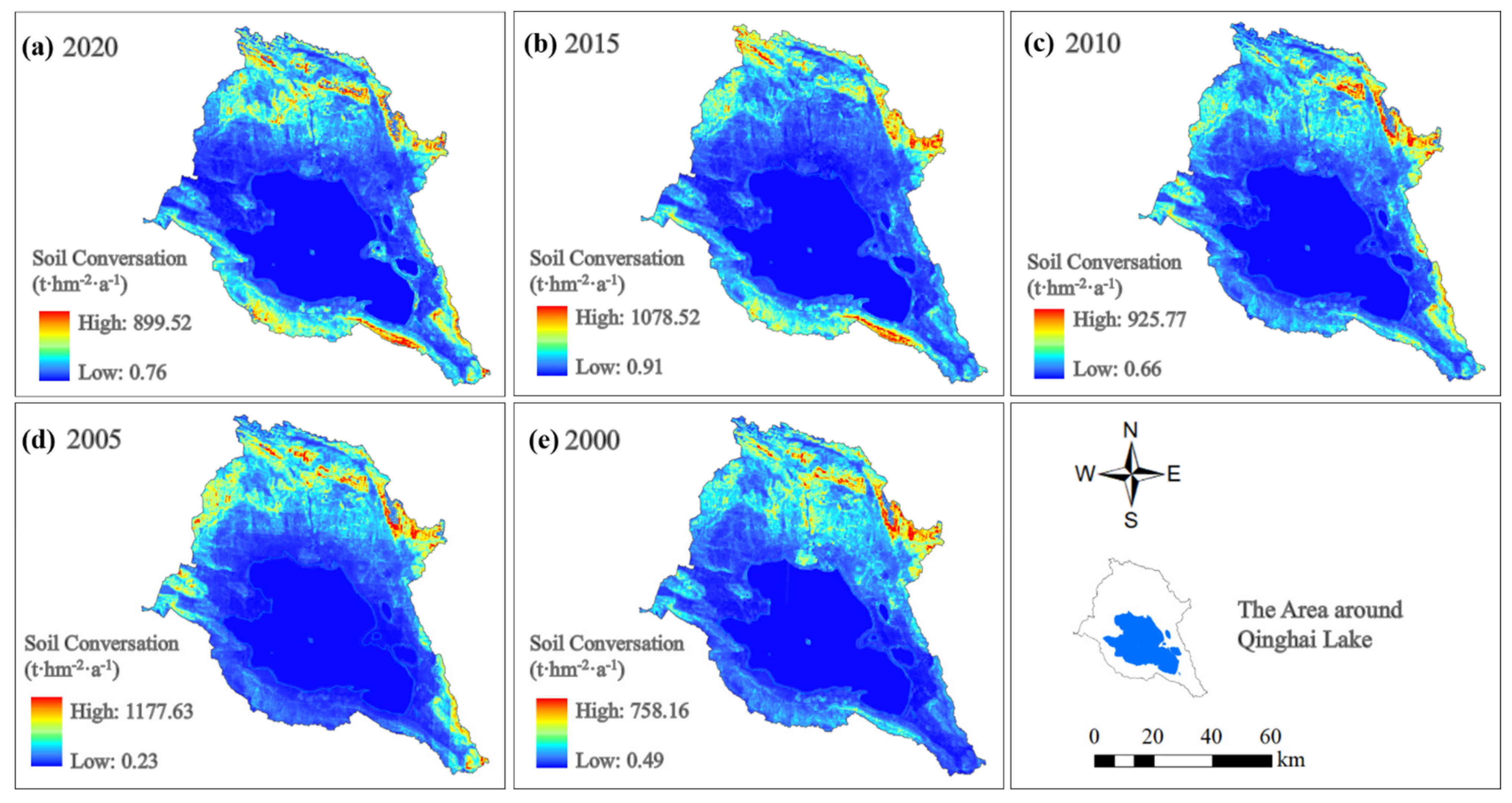
2.2.2. Soil Conservation

The InVEST, a soil conservation module is based on the revised universal soil loss equation (RUSLE) to estimate the soil conservation of each raster in the study area by subtracting the actual soil erosion from the potential soil loss. The formula is:

$${\mathit{RKLS}}_i=R_i{\times K}_i{\times \mathit{LS}}_i$$

(4)

$${\mathit{USLE}}_i=R_i{\times K}_i{\times \mathit{LS}}_i{\times C}_i{\times P}_i$$

(5)

$${\mathit{SD}}_i={\mathit{RKLS}}_i-{\mathit{USLE}}_i$$

(6)

where RKLS_i represents the amount of soil erosion of bare land on each raster i (t·hm⁻²·a⁻¹), and USLE_i is the amount of soil erosion of each raster i under the action of vegetation cover management factors and water and soil conservation measures factors (t·hm⁻²·a⁻¹); SD_i is the actual soil conservation (t·hm⁻²·a⁻¹); R_i is rainfall erosivity factor (MJ·mm·hm⁻²·h⁻¹·a⁻¹), which is calculated by Wischmeier’s monthly scale formula [42]; K_i is the soil erodibility factor (t·hm²·h·hm⁻²·MJ⁻¹·mm⁻¹), which is localized and corrected by EPIC model; LS_i is the slope length and slope factor; C_i is the vegetation cover management factor, referring to the research of Cai et al. [43]; P_i is the factor of water and soil conservation measures.

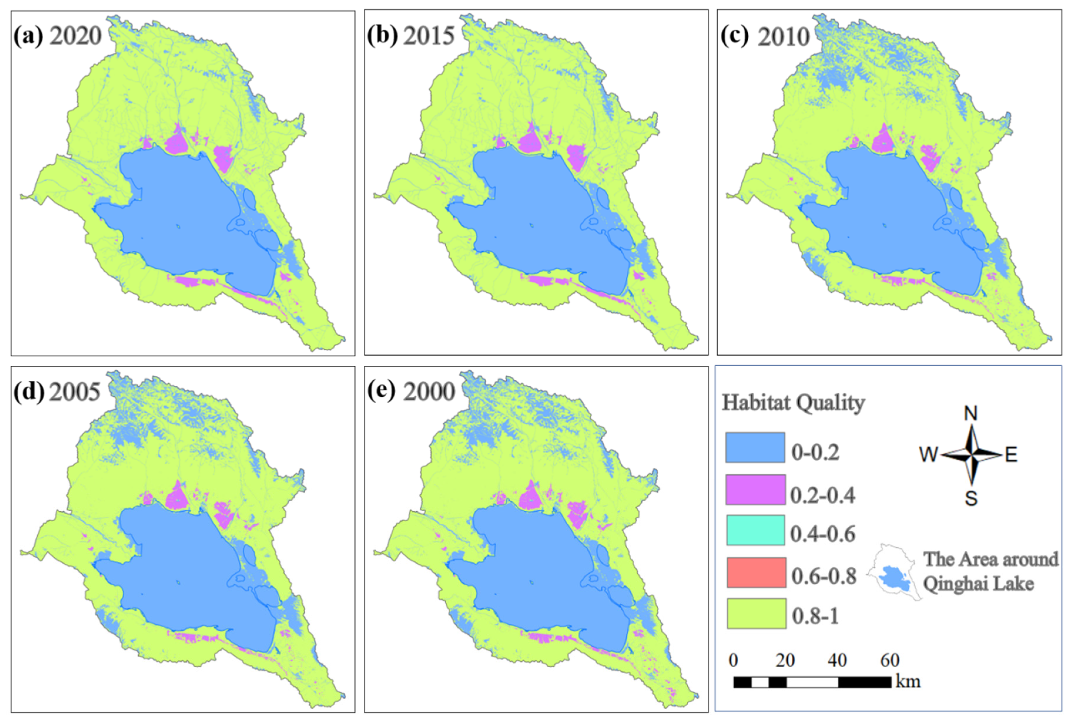
2.2.3. Habitat Quality

Based on land use data and threat source data, the InVEST model calculates the habitat quality score of each raster. The score is between 0 and 1, the larger the value, the better the habitat quality. In this study, cultivated land, urban and built-up land, unused land (currently unused land, including hard-to-use land, sandy land, Gobi, saline-alkali land, bare land, etc.), and roads were selected as threat source data, and the habitat quality parameter table was constructed (

Table A1. Land use classification and its specific description.

Land Use Types	Description
Cultivated land	It refers to the land for planting crops, including mature cultivated land, newly opened wasteland, leisure land, rotation land, and grass field rotation land. Agricultural fruit, mulberry, and forestry land mainly for planting crops. Beaches and tidal flats that have been cultivated for more than three years.
Woodland	It refers to the forest land for growing trees, shrubs, open woodlands, nurseries, and various gardens.
Grassland	It refers to all kinds of grasslands mainly growing herbaceous plants with a coverage of more than 5%, including shrub grassland dominated by grazing and open forest grassland with a canopy density of less than 10%.
Waters	It refers to the natural land water area and the land for water conservancy facilities, including rivers, lakes, reservoirs, ponds, and beaches.
Built-up land	It refers to urban and rural residential areas, factories, and mines independent of cities and towns, large industrial areas, quarries, traffic roads, and special land.
Unused land	It refers to currently unused land, including hard-to-use land, sandy land, Gobi, saline-alkali land, bare land, etc.

). Finally, the habitat quality module was run to obtain the habitat quality score of each raster of the study area in Qinghai Lake. The specific formula is as follows:

$$Q_{\mathit{ij}}{=H}_j\left[1-\frac{D_{\mathit{ij}}^z}{D_{\mathit{ij}}^z{+k}^z}\right]$$

(7)

$$D_{\mathit{ij}}={\displaystyle \sum }_{r=1}^R{\displaystyle \sum }_{p=1}^{P_r}\left(\frac{w_r}{{{\displaystyle \sum }}_{r=1}^R{w}_r}\right)r_p{i}_{\mathit{rip}}{\beta }_i{S}_{\mathit{jr}}$$

(8)

where Q_ij is the habitat quality of each raster i; H_j is the habitat suitability of land use type j; D_ij is the habitat degradation degree of each raster i; k is the semi saturation constant 0.5; Z is the default parameter 2.5; R is the number of threat factors; P_r is the total number of each raster of threat factor r; W_r is the weight of threat factor r; rp is the threat intensity; i_rip represents the threat degree of rp to each raster i; β_i represents the accessibility of i; S_jr is the sensitivity of land use type j to threat factor r.

2.3. Random Forest

RF is a multi-decision tree integrated model, which can explain the influence degree of several independent variables (x₁, x₂, …, x_k) on dependent variable Y. Assuming that the dependent variable Y has n observations and k relevant independent variables, the random forest regression model randomly and independently extracts sample data (in bag samples) to build a decision tree, and the remaining data (out of bag samples, OOB) is used as the test set. Finally, the tree with the highest degree of repetition is selected as the result [44]. This renders the model to well predict the degree of influence of multiple explanatory variables, have a good tolerance for noise and outliers, and avoid overfitting to a certain extent. The RF model uses the percentage increase of mean square error (% Inc MSE) to evaluate the influence of independent variables on dependent variables. The greater the value, the greater the importance of independent variables.

The decision tree model is constructed, and the OBB mean square error matrix of random replacement is calculated as follows:

$$\left[\begin{array}{cccc}{\mathit{MSE}}_{11}& {\mathit{MSE}}_{12}& \cdots & {\mathit{MSE}}_{1\mathit{ntree}}\\ {\mathit{MSE}}_{21}& {\mathit{MSE}}_{22}& \dots & {\mathit{MSE}}_{2\mathit{tree}}\\ ⋮& ⋮& ⋮& ⋮\\ {\mathit{MSE}}_{m1}& {\mathit{MSE}}_{m2}& \cdots & {\mathit{MSE}}_{\mathit{mtree}}\end{array}\right]$$

(9)

The importance of calculating scores is as follows:

$${\mathit{score}}_x{=S}_E^{-1}\frac{{{\displaystyle \sum }}_{r=1}^{n_{\mathit{tree}}}{\mathit{MSE}}_r-{\mathit{MSE}}_{\mathit{pr}}}{n_{\mathit{tree}}},(1\le p\le m)$$

(10)

where n is the number of original data samples; m is the number of variables.

Based on the availability of data and empirical judgment, this study selected eight natural and socio-economic factors, including precipitation (pre), temperature (tem), altitude (DEM), slope, human footprint (HF), gross domestic product (GDP), population density (POP) and normalized difference vegetation index (NDVI). Taking eight influencing factors as independent variables and three ecosystem provisioning services as dependent variables, the RF model between natural and socio-economic factors and ecosystem services was constructed in the “random forest” package of R language.

2.4. The Geographically and Temporally Weighted Regression Model

Geographically weighted regression (GWR) is a classical model for the study of spatial heterogeneity, which requires a certain number of samples, but in reality, the sample size of cross-sectional data is limited, which often affects the results of the model. However, the GTWR model introduces the time dimension into the GWR model, which can obtain the dual information of time and space, making the estimation results more effective. The expression for the GTWR model is as follows:

$${Y=\beta }_0(u_i,v_i,t_i)+{\displaystyle \sum }_{k=1}^p{\beta }_k(u_i,v_i,t_i)x_{\mathit{ik}}{+\epsilon }_i$$

(11)

where u_i and v_i are the coordinates for the longitude and latitude, respectively, of raster i; t_i is the time coordinate of raster i; β₀ is the regression constant; β_k is the kth regression parameter; x_ik is the value of independent variable x_k in raster i; ε_i is the random error term.

Based on the results of the RF model, this study selected the first three factors affecting each ecosystem service as the driving factors. Based on the GTWR model and taking three ecosystem services as dependent variables, the regression coefficient of each driving factor was calculated to reflect the spatial differentiation of driving factors on ecosystem services.

2.5. Data Sources

Precipitation and temperature data were obtained from the China Meteorological data network (http://data.cma.cn, accessed on 28 August 2021), the source of MOD 16A2 remote sensing data was evapotranspiration (https://ladsweb.modaps.eosdis.nasa.gov, accessed on 28 August 2021), and the temporal and spatial resolution were 8 d 500 m. NDVI was from the US Geological Survey (USGS) land process Distributed Data Archive Center (https://lpdaas.usgs.gov, accessed on 28 August 2021) MOD13 Q1 data. Land-Use and Land-Cover Change (LUCC) data were originally downloaded from Geospatial Data Cloud (http://www.gscloud.cn, accessed on 28 August 2021); then, conducted radiometric calibration, atmospheric correction, and image fusion using GEE (Google Earth Engine) platform; finally, obtained by visual interpretation using ArcGIS. Soil data, including soil texture, organic matter content, and bulk density, were derived from the soil series survey of China—Qinghai volume and the Chinese soil data set of the Food and Agriculture Organization of the United Nations (FAO) and Harmonized World Soil Database (HWSD). GDP and POP data were from the resource and environment data center of the Chinese Academy of Sciences (http://www.resdc.cn/data, accessed on 7 May 2021). HF comes from the human footprint data set of the Qinghai Tibet Plateau calculated by Duan et al. [45]. This paper selected the data from 2000, 2005, 2010, 2015, and 2020 for research (

Table 1. Information of data used in this study.

Data Type	Unit	Resolution/Scale	Data Sources
Monthly precipitation	mm	1 km	http://data.cma.cn (accessed on 28 August 2021)
Average monthly temperature	°C	1 km	http://data.cma.cn (accessed on 28 August 2021)
Evapotranspiration	mm	500 m	https://ladsweb.modaps.eosdis.nasa.gov (accessed on 28 August 2021)
Normalized Difference Vegetation Index	/	250 m	https://lpdaas.usgs.gov (accessed on 28 August 2021)
Digital Elevation	m	30 m	Shuttle Radar Topography Mission
Soil texture	%	1 km	Harmonized World Soil Database
Soil organic matter	%	1 km	Harmonized World Soil Database
Soil bulk density	g·cm−3	1 km	Harmonized World Soil Database
Land-Use and Land-Cover Change	/	Type Value	Remote sensing interpretation
Gross Domestic Product	Ten thousand yuan /km2	1 km	http://www.resdc.cn/data (accessed on 7 May 2021)
Population Density	Person/km2	1 km	http://www.resdc.cn/data (accessed on 7 May 2021)
Human Footprint	/	1 km	https://data.tpdc.ac.cn/ (accessed on 7 May 2021)

).

3. Result

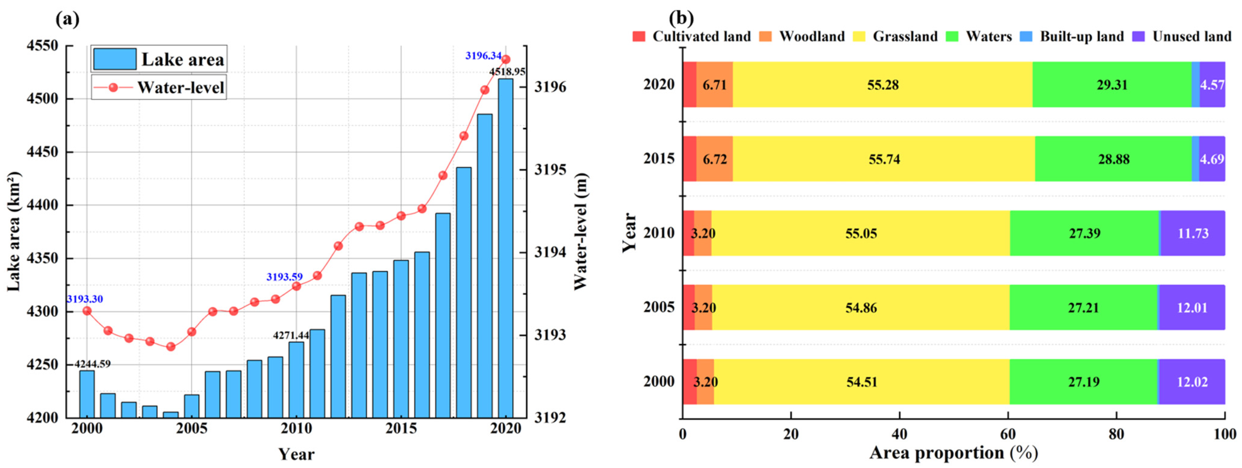
3.1. Temporal Changes of Ecosystem Provisioning Services around Qinghai Lake

The three ecosystem services of water yield, soil conservation, and habitat quality in the study area in 2000, 2005, 2010, 2015, and 2020 were calculated using the InVEST model (

Table 2. Changes in three ecosystem services from 2000 to 2020.

Year	Ecosystem Services Per Unit Area			Total Ecosystem Services
	WY (mm)	SC (t·hm−2·a−1)	HQ	WY (×108 m3)	SC (×108 t)	HQ (×106)
2020	349.27	271.82	0.66	56.55	1.58	11.93
2015	377.51	341.89	0.67	61.12	1.86	12.00
2010	367.60	285.84	0.63	59.52	1.60	11.30
2005	444.68	331.39	0.63	72.00	1.74	11.27
2000	338.40	230.05	0.62	54.79	1.20	11.23

Note: WY, SC, and HQ refer to water yield, soil conservation, and habitat quality respectively.

). In 2000–2020, the total water yield and average water yield depth in the study area showed a fluctuating trend of “increase-decrease-increase-decrease”. It showed an overall increasing trend, and the total water yield increased from 54.79 × 10⁸ m³ to 56.55 × 10⁸ m³, with an increase of 3.21%. The maximum average water yield depth in 2005 was 444.68 mm, and the total annual water yield increased the most from 2000 to 2005, with a total increase of 17.21 × 10⁸ m³ by 2005, and the average water yield depth increased by 106.28 mm, due to the increase of precipitation and river runoff in the study area after 2005; the supply of water resources also has an obvious increasing trend. In 2005–2020, the average depth of water yield first decreased by 17.33%, then increased by 2.70%, and then decreased by 7.48%. The overall change in the trend of soil conservation services in the study area in 2000–2020 was consistent with that of water yield services, and soil conservation service values were 0.23 to 1177.63 t·hm⁻²·a⁻¹ in 2000–2020. The soil conservation per area increased from 230.05 t·hm⁻²·a⁻¹ in 2000 to 331.39 t·hm⁻²·a⁻¹ in 2005, then decreased to 285.84 t·hm⁻²·a⁻¹ in 2010 and increased to 341.89 t·hm⁻²·a⁻¹ in 2015. In 2000–2020, the average soil conservation in the study area was 1.60 × 10⁸ t, which was a 31.67% increase in 2020 compared to that in 2000. The habitat quality score of the study area showed a yearly increasing trend from 2000–2015 (Table 2), which decreased by only 0.60% from 2015 to 2020, with a high multi-year average of 0.64.

3.2. Spatial Changes in Ecosystem Provisioning Services around Qinghai Lake

Spatially, there were significant differences in water yield service areas (Figure 2). The water yield was less in and around the Qinghai Lake area, and there were more watershed areas in the north and the boundary of the region, showing that in the surrounding high Lake area, the north and east are higher and the south and west are relatively lower, consistent with the distribution characteristics of rainfall in this area.

The spatial distribution characteristics of soil conservation services were low in the lake area and high around the area, which was consistent with the distribution pattern of water production services (Figure 3). The areas with high values of soil conservation services were mainly distributed in the marginal areas of the region. Concurrently, with the increase in precipitation in the region, vegetation coverage increased, and the capacity of soil conservation services increased. The lake area is mainly distributed by water, and there is almost no soil evolution, resulting in the weakening of soil conservation service capacity. The soil conservation value of the lake center was not zero due to the existence of Haixin Mountain in Qinghai Lake. There might be a large amount of sediment below the water body, which was also a way of soil conservation and caused the soil conservation value of the water body in Qinghai Lake to not be zero [46].

The overall habitat of the study area exhibited fairly obvious spatial differentiation (Figure 4). Warm grasslands around the lake, alpine meadows, wetlands, and forest areas have high vegetation coverage and low intensity of human disturbance, so the habitat quality score should be high. However, due to the intensive population and strong human activities in the peripheral areas around the lake, the connectivity of the habitat has been damaged, which led to poor habitat quality.

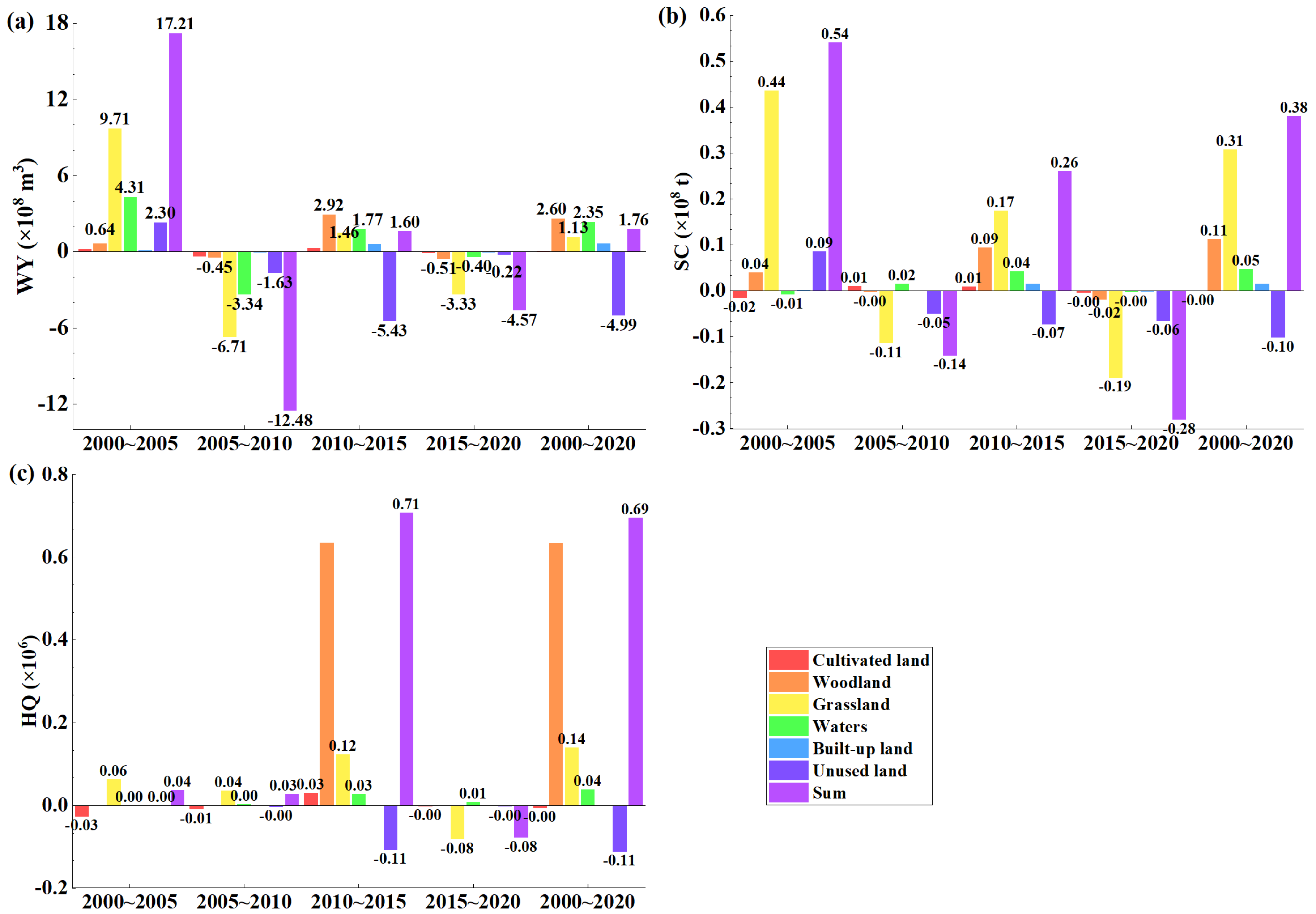
3.3. Changes in Ecosystem Provisioning Services in Different Land Use Types

In the past 15 years, the water level of Qinghai Lake has been rising continuously [47] and the water area in the study area has been increasing (Figure 5), causing a change in the area of other land types and ecosystem services of the whole region. To explore the change in ecosystem services in different land types after the rise in water level and whether it showed the trend of increasing ecosystem services in water areas and decreasing ecosystem services in other land types, i.e., one fades and the other fades, this study analyzed the zoning statistics of three ecosystem services: water yield, soil conservation, and habitat quality through five periods of land use data in 2000–2020, to obtain the change in ecosystem services per unit area on different land types (Figure 6) and the overall change in total ecosystem services (Figure 7).

Taking the most significant stage of water level increase (2015–2020) as an example, this study analyzed the changes in the area of various types of land after the rise in water level in Qinghai Lake. In 2015–2020, the expansion of water was over 77.22 km² of grassland (75.84% of the increased area comes from grassland), 18.88 km² of unused land, 4.02 km² of woodland, 1.35 km² of built-up land, and 0.35 km² of cultivated land (

Table 3. Area transfer matrix of various categories in 2015–2020 (km²).

2015–2020	Cultivated Land	Woodland	Grassland	Waters	Built-Up Land	Unused Land	Loss-2015
Cultivated land		0.03	3.87	0.35	6.41	0.01	10.67
Woodland	0.05		52.92	4.02	1.18	2.01	60.18
Grassland	4.86	54.08		77.22	58.16	18.13	212.45
Waters	0.02	2.59	22.71		1.26	5.32	31.89
Built-up land	3.58	0.95	42.10	1.35		0.26	48.24
Unused land	0.02	2.13	20.86	18.88	0.48		42.37
Gain-2015	8.53	59.78	142.45	101.82	67.49	25.72	405.81
Net changes	−2.14	−0.40	−69.99	69.93	19.25	−16.65

). In general, the area of water and built-up land showed a net increase, while the area of other land types showed a net decreasing trend. However, the ecosystem services of waters, built-up land, grassland, and other land types showed a downward trend in 2015–2020 (Figure 6 and Figure 7). If this increasing trend of water continues, the change in land area and the related loss of ecosystem services are also expected to increase in the future.

In 2000–2020, the water yield services per unit area of various types showed a “rise- decline-rise-decline” trend, the soil conservation services per unit area of cultivated land and waters showed a “decline-rise-decline-rise” trend, and the habitat quality services per unit area of cultivated land, woodland, grassland, and waters decreased in 2000–2005, and all land use types essentially stabilized between 2010 and 2020. From the same land type (Figure 6), the water yield, soil conservation, and habitat quality service of woodland were the highest, the water yield and soil conservation service of waters were the lowest, and the habitat quality service of built-up land was the lowest. Taking 2020 as an example, in different land use types (Figure 7), the order of total water yield services was: grassland > waters > woodland > unused land > cultivated land > built-up land. The total amount of soil conservation services was: grassland > woodland > unused land > waters > cultivated land > built-up land, and the total amount of habitat quality services was: woodland > grassland > cultivated land > waters > unused land > built-up land.

4. Discussion

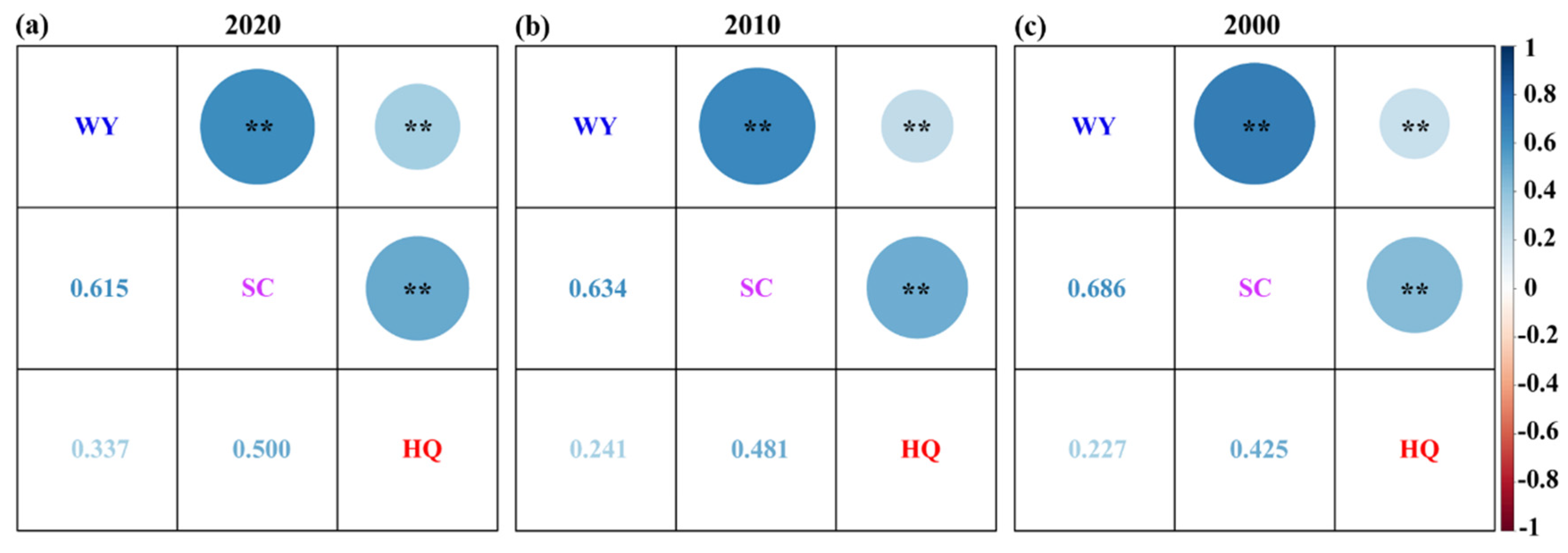
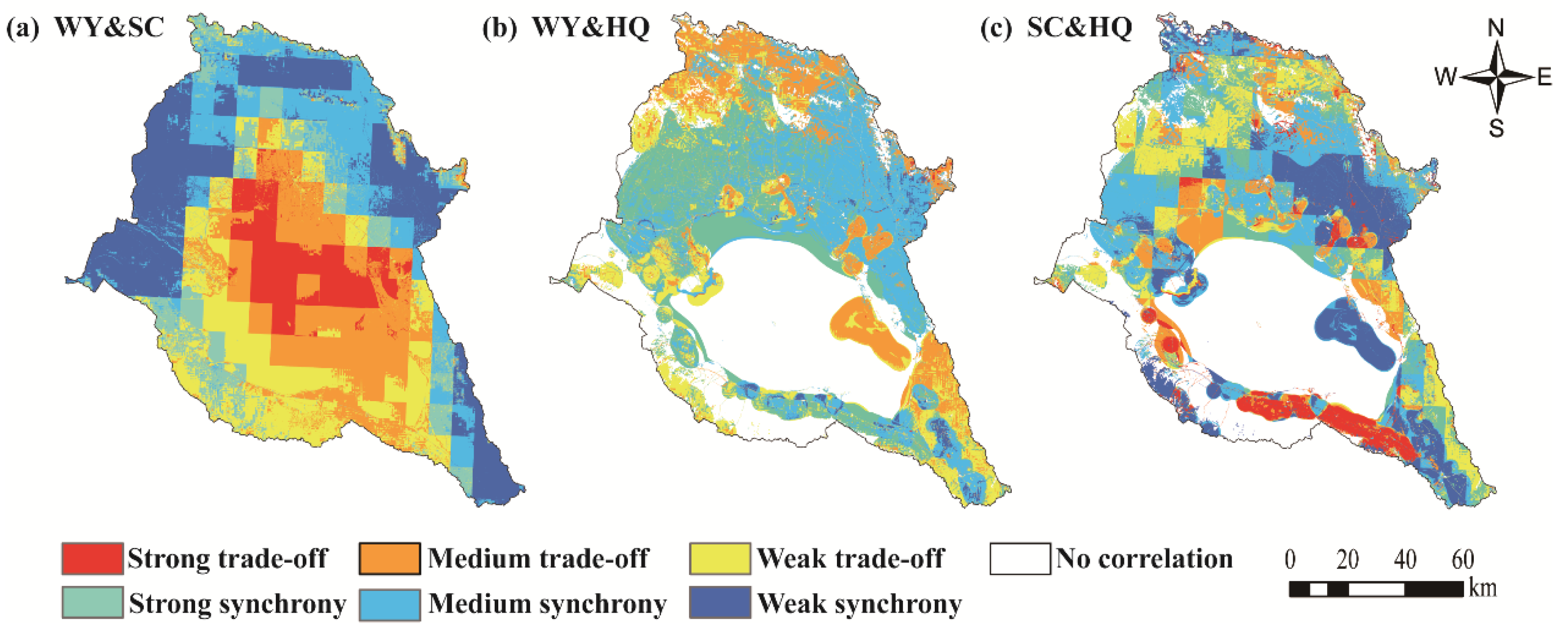
4.1. Trade-Off and Synchrony among Ecosystem Provisioning Services

The R language “corrgram” function was used to analyze the trade-off and synchrony among three ecosystem services, including water yield, soil conservation, and habitat quality. By establishing the Spearman correlation matrix for different ecosystem services (Figure 8), the three ecosystem services in the study area showed a significant positive correlation, that is, synchrony from 2000 to 2020. The correlation coefficient r between water yield and soil conservation was the highest, which was greater than 0.6, indicating a strong synchronous relationship between them. The reason was that vegetation in areas with high water yields generally grew well and had a strong soil conservation capacity. There was a synchronous relationship between water yield and habitat quality, and the correlation coefficient increased from 0.227 in 2000 to 0.337 in 2020. The relationship between soil conservation and habitat quality was found to change from weak synchrony to strong synchrony because the area with good habitat quality has high vegetation coverage and is not prone to soil erosion.

The spatial correlation level of three ecosystem services was analyzed based on the pixel scale and produced the spatial distribution map of ecosystem service trade-off and coordination by ArcGIS 10.6 software [30] (Figure 9 and

Table A2. Description of trade-off and synchrony relationship.

Correlation Coefficient	Trade-Off and Synchrony
0.7~1	Strong synchrony
0.3~0.7	Medium synchrony
0~0.3	Weak synchrony
0	No correlation
−0.3~0	Weak trade-off
−0.7~−0.3	Medium trade-off
−1~−0.7	Strong trade-off

). Synchrony was observed between water yield and soil conservation spatially (50.02% area), which was mainly concentrated in the north and southeast of the region and the marginal area of Qinghai Lake area, and the strong trade-off was distributed in the Qinghai Lake area. The spatial relationship between water yield and habitat quality was mainly synchrony (43.04% area), and the synchronous areas were mainly concentrated in the north of the region and the south edge of the lake area, while the other areas showed no correlation (31.21% area), and the trade-off relationship was sporadically distributed in the north and southeast of the region. The interaction between soil conservation services and habitat quality services was also dominated by synchrony (43.66% area), with a complex spatial distribution pattern, and the synchrony and trade-off were spatially intersected. The synchrony was mainly distributed in the north and south edge of the lake area, and the strong trade-off was mainly distributed in the south edge of the lake area.

4.2. Trade-Off and Synchrony of Ecosystem Provisioning Services in Different Land Types

The relationship among the three ecosystem services in each land use type was analyzed (Figure 10). Among different land types, the relationship between water yield and soil protection services was dominated by synchrony. Among them, the synchrony of woodland, grassland, built-up land, and unused land was more than 50%. The highest proportion of synchrony was that of woodland, with a synchrony area of 83.23%. The cultivated land and waters mainly exhibited a trade-off relationship, and the trade-off relationship of the water ecosystem accounted for 92.48%. The relationship between water yield and habitat quality services also was mainly synchrony. Among them, the proportion of synchronous relationship area of cultivated land was as high as 80.36%, and that of built-up land was as low as 58.04%. Only in woodland and unused land, the relationship between ecosystem services was mainly a trade-off.

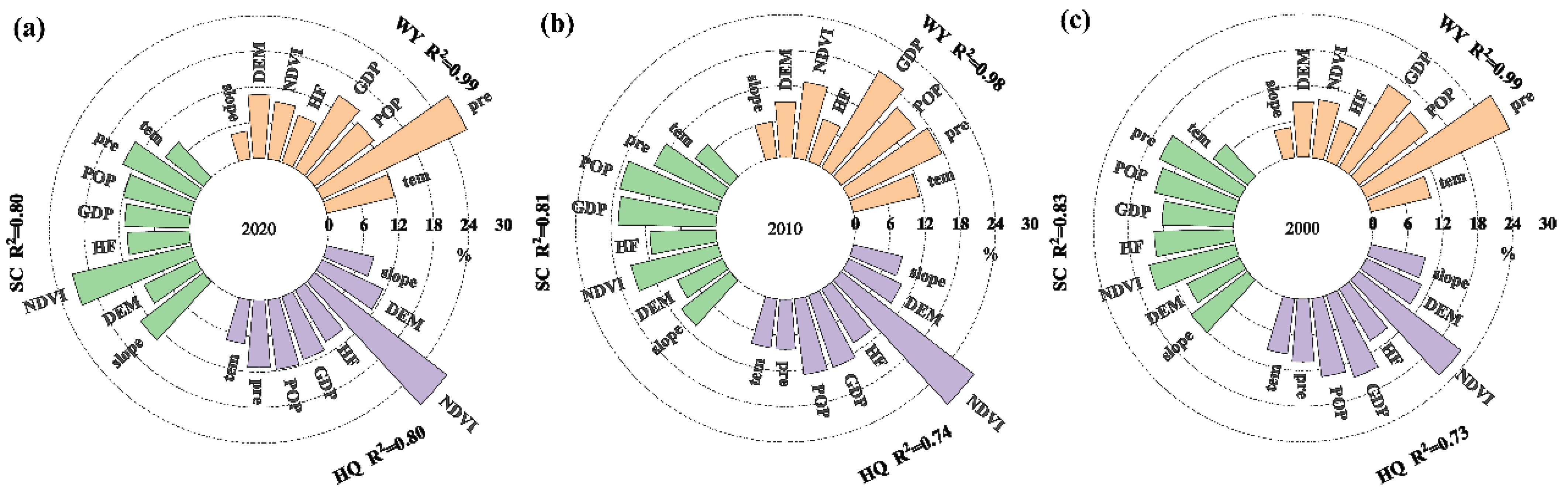
4.3. Influencing Factors of Ecosystem Provisioning Services

Based on the RF model, the social-ecological environment factors of three ecosystem services in 2000–2020 were statistically modeled; the goodness of fit R² was more than 0.7, indicating that the model can well fit the relative impact of various factors on the temporal and spatial distribution of ecosystem services (Figure 11).

The results showed that the water yield service in the study area was mainly affected by climate factors (mainly affected by GDP factors in 2010); particularly, the proportion of precipitation factors in 2020 was up to 27.48%, followed by POP and GDP, temperature, while DEM and NDVI contribute less, and HF and slope had the weakest impact. Since precipitation was one of the most important factors to determine the surface runoff when the precipitation exceeded the interception of the underlying surface, the surface runoff was generated, and the number of water resources in the region also increased.

In 2000–2020, soil conservation services were mainly affected by NDVI and precipitation. In 2020, the proportion of NDVI and precipitation was 20.93% and 13.85%, respectively. The high-value areas of soil conservation services were basically consistent with the high-value areas of NDVI and precipitation. Appropriate precipitation can promote vegetation growth and improve vegetation coverage and soil conservation capacity. However, when the precipitation exceeded a certain threshold, it scoured the soil and weakened the soil conservation function, causing the soil conservation service to be more easily affected by GDP and POP in 2010.

The explanation degree of each factor to the spatial differentiation of habitat quality was NDVI > POP > DEM > pre > GDP > HF > slope > tem. The impact of NDVI on the watershed habitat quality service was higher than other terrains, climate, and human activity factors, indicating that the higher the vegetation coverage, the higher the habitat quality service provided by the region.

Based on the RF and GTWR models, precipitation was estimated to play a leading role in water conservation services from 2000 to 2020, which was related to the decline considering the background of warming and humidification in the Qinghai Tibet Plateau, and increase in water volume, river runoff and water resources in the region [48]. The existing research results show that human activities have a great impact on the spatial distribution of ecosystem services [49], but the correlation of POP and GDP on various ecosystem services (except soil conservation services) is not dominant so far. Li et al., also showed that the overall ecological environment of the Qinghai Tibet Plateau was less affected by human activities in 1990–2020 [50]. As a controllable management factor, NDVI played an important role in the feedback on soil conservation and habitat quality service supply [51].

4.4. Spatial Differentiation of Driving Factors of Ecosystem Provisioning Services

To intuitively reflect the spatial differentiation of driving factors on ecosystem services, in this study, we selected the first three factors affecting ecosystem services as driving factors and determined their regression coefficients based on the GTWR model to make the spatial differentiation map (Figure 12). The results showed that the adjusted R² was more than 0.6 and the p-value was less than or equal to 0.05, indicating that the GTWR model had great goodness of fit, and confirmed that the selected driving factors had explanatory power on ecosystem services. The results also showed that precipitation had a significant impact on the spatial distribution of water yield services (Figure 12), consistent with the research results of Yang et al. [52], showing an increasing trend from northeast to southwest. POP showed a positive impact in the lake area while a negative impact around the lake area; its impact in the north and southeast of the region was significant, indicating that the water yield services in areas with low population density were higher. The spatial distribution difference of GDP on water yield services was obvious. Except for the northern part of the region, the other areas exhibited a mainly negative impact, indicating that the higher the GDP, the lower the water conservation services. NDVI had a positive impact on soil conservation services, with obvious spatial differences, which were manifested as a distribution from northwest to southeast, with a low correlation between the lake area and the surrounding area. Precipitation was an important factor affecting vegetation coverage, which was mainly positive in the northeast of the region. The slope was mainly positive in the north of the region. The positive effect of NDVI on habitat quality service was primary, which is generally characterized by circular distribution centered on the Qinghai Lake area. POP had both positive and negative effects in the east of the region. The reason is that POP, as a manageable external factor, has a strong ability to transform the surface in areas. The land use mode had an absolute influence on the spatial distribution of habitat quality, and it changed the surface vegetation coverage and then affected the spatial distribution of habitat quality. Finally, DEM mainly had a negative impact on habitat quality service and had a positive impact only in the lake area.

4.5. Reliability and Limitation

Studies about ecosystem services of the Qinghai Lake are mainly on a short time scale and focus on ecosystem service value calculation [53,54,55], lacking the long-term and continuous time series spatial and temporal change analysis and ecosystem service research based on material quality [56,57]. The multi-year average of soil conservation per unit area in the study area simulated by the InVEST model in 2000–2020 was 292.20 t·hm⁻²·a⁻¹, which was close to the multi-year average (365.91 t·hm⁻²·a⁻¹) of the whole Qinghai Lake Basin calculated by Han, using the InVEST model in 2000–2018 [58]. The total amount of soil conservation and water yield showed a fluctuating and increasing trend. The water yield and habitat quality service space in this study area showed an increasing trend from the center to the edge; the findings were consistent with the simulation results of Lian et al. [59], which confirmed the reliability of simulation results obtained using the InVEST model.

The relationship between ecosystem services, water yield, soil conservation, and habitat quality services were synchronous. The relationship between ecosystem services in a single year was different from that in the past 20 years; weak synchrony was observed in a single year, the interannual synchrony fluctuated with each other, and the soil conservation and habitat quality changed greatly over the years. The synchrony between water yield and soil conservation in the study area was the main relationship. The increase in precipitation promoted vegetation development and enhanced the soil conservation capacity. This conclusion was basically consistent with the research of Bennett et al. [60].

This study and the methods used had limitations and uncertainties. This study only simulated three ecosystem services but did not simulate water purification, carbon storage, windbreak, sand fixation, biodiversity, and other services, which led to the lack of ecosystem service assessment comprehensively. The study did not consider soil conservation services in specific areas (such as beneath water bodies) due to the limitations of the survey in natural conditions, then we just did homogenization temporarily, which was the point of further research and deserves more attention. The calculation and selection of biophysical parameters of each module of InVEST model in this study were combined with the characteristics of the study area, referring to the existing calculation methods and relevant literature. However, the determination of various parameters (vegetation root depth in the water yield module, soil, and water conservation measure factors in the soil conservation module, the sensitivity of land use type to threat sources in the habitat quality module, etc.) still has uncertainties, which affects the simulation accuracy. We set habitat quality measures to a low value in the lake area, and this was not because it had no value or low value, but because it was limited by aquatic ecological environment survey and lack of aquatic biological data. Therefore, it is necessary to comprehensively evaluate the ecosystem services in the region in the future. When localizing and correcting the model parameters, it is also important to carry out field observation and experimental analysis according to the study area characteristics, for verifying the parameters and determining their rationality, which can improve the simulation accuracy of the model.

5. Conclusions

Based on the InVEST-RF-GTWR combined method, the spatial and temporal changes in water conservation, soil conservation, and habitat quality in 2000–2020 were analyzed. It not only evaluated the change of ecosystem provisioning services of different land types with the rise in water level of Qinghai Lake but also explored their synchrony trade-off relationship and the driving factors. This method can be taken into account in other ecosystem services evaluation studies.

Our results revealed that the water yield, soil conservation, and habitat quality of the area around Qinghai Lake showed a fluctuating rise in 2000–2020. The three ecosystem provisioning services increased in 2000–2005, while decreased in 2005–2020 with the rising water level. There was strong synchrony between water yield and soil conservation services, weak synchrony between water yield and habitat quality, and weak synchrony between soil conservation and habitat quality. The ecosystem services among different land use types presented a synchronous relationship in 2000–2020. For the same land use type, only the ecosystem provisioning services on the grassland showed a synchronous relationship.

Precipitation factors had the most significant impact on water yield, and NDVI had the most significant effect on soil conservation and habitat quality services, meanwhile, ecosystem provisioning services have also been weakened by human activities. In the future, assuming that the water level continues to rise, the loss of ecological services will increase. This study clarified the spatial and temporal pattern and evolution trend of ecosystem services around Qinghai Lake and provided a basis for proposing strategies for addressing global climate change.

References

1. Verpoorter, C.; Kutser, T.; Seekell, D.A.; Tranvik, L.J. A global inventory of lakes based on high-resolution satellite imagery. Geophys. Res. Lett. 2014, 41, 6396–6402. [Google Scholar] [CrossRef]
2. Wang, J.; Song, C.; Reager, J.T.; Yao, F.; Famiglietti, J.S.; Sheng, Y.; MacDonald, G.M.; Brun, F.; Schmied, H.M.; Marston, R.A.; et al. Recent global decline in endorheic basin water storages. Nat. Geosci. 2018, 11, 926–932. [Google Scholar] [CrossRef]
3. Alsdorf, D.E.; Rodríguez, E.L.; Lettenmaier, D.P. Measuring surface water from space. Rev. Geophys. 2007, 45, RG2002. [Google Scholar] [CrossRef]
4. Costanza, R.; Arge, R.; Groot, R.D.; Farber, S.; Grasso, M.; Hannon, B.; Limburg, K.; Naeem, S.; Neill, R.V.; Paruelo, J.; et al. The value of the world’s ecosystem services and natural capital. Nature 1997, 387, 253–260. [Google Scholar] [CrossRef]
5. Vitousek, P.M.; Mooney, H.A.; Lubchenco, J.; Melillo, J.M. Human Domination of Earth’s Ecosystems. Science 1997, 277, 494–499. [Google Scholar] [CrossRef]
6. Su, X.; Bo, Z.; Huang, W.; Su, X.; Lei, S. Effects of the Three Gorges Dam on preupland and preriparian drawdown zones vegetation in the upper watershed of the Yangtze River, P.R. China. Ecol. Eng. 2012, 44, 123–127. [Google Scholar] [CrossRef]
7. Qi, Y.; Lian, X.; Wang, H.; Zhang, J.; Yang, R. Dynamic mechanism between human activities and ecosystem services: A case study of Qinghai Lake watershed, China. Ecol. Indic. 2020, 117, 106528. [Google Scholar] [CrossRef]
8. Gu, X.; Long, A.; Liu, G.; Yu, J.; Wang, H.; Yang, Y.; Zhang, P. Changes in ecosystem service value in the 1 km lakeshore zone of Poyang Lake from 1980 to 2020. Land 2021, 10, 951. [Google Scholar]
9. Paterson, A.M.; Rühland, K.M.; Anstey, C.V.; Smol, J.P. Climate as a driver of increasing algal production in lake of the woods, Ontario, Canada. Lake Reserv. Manag. 2017, 33, 403–414. [Google Scholar] [CrossRef]
10. Yang, G.; Zhang, Q.; Wan, R.; Lai, X.; Jiang, X.; Li, L.; Dai, H.; Lei, G.; Chen, J.; Lu, Y. Lake hydrology, water quality and ecology impacts of altered river-lake interactions: Advances in research on the middle Yangtze river. Hydrol. Res. 2016, 47, 1–7. [Google Scholar] [CrossRef]
11. Mekuria, W.; Diyasa, M.; Tengberg, A.; Haileslassie, A. Effects of long-term land use and land cover changes on ecosystem service values: An example from the Central Rift Valley, Ethiopia. Land 2021, 10, 1373. [Google Scholar] [CrossRef]
12. Lavorel, S.; Grigulis, K.; Lamarque, P.; Colace, M.P.; Garden, D.; Girel, J.; Pellet, G.; Douzet, R. Using plant functional traits to understand landscape distribution of multiple ecosystem services. J. Appl. Ecol. 2011, 99, 135–147. [Google Scholar] [CrossRef]
13. Chapin, F.S.; Matson, P.A.; Mooney, H.A. Principles of Terrestrial Ecosystem Ecology; Springer: New York, NY, USA, 2011. [Google Scholar]
14. Darvill, R.; Lindo, Z. The inclusion of stakeholders and cultural ecosystem services in land management trade-off decisions using an ecosystem services approach. Landsc. Ecol. 2016, 31, 533–545. [Google Scholar] [CrossRef]
15. Millennium Ecosystem Assessment. Ecosystems and Human Well-Being: Synthesis; Island Press: Washington, DC, USA, 2005. [Google Scholar]
16. Angradi, T.R.; Launspach, J.J.; Bolgrien, D.W.; Bellinger, B.J.; Starry, M.A.; Hoffman, J.C.; Trebitz, A.S.; Sierszen, M.E.; Hollenhorst, T.P. Mapping ecosystem service indicators in a Great Lakes estuarine Area of Concern. J. Great Lakes Res. 2016, 42, 717–727. [Google Scholar] [CrossRef]
17. Cui, L. Evaluation of functions of Poyang Lake ecosystem. Chin. J. Ecol. 2004, 23, 47–51. [Google Scholar]
18. Schirpke, U.; Tasser, E.; Leitinger, G.; Tappeiner, U. Using the ecosystem services concept to assess transformation of agricultural landscapes in the European Alps. Land 2022, 11, 49. [Google Scholar] [CrossRef]
19. Shui, W.; Wu, K.; Du, Y.; Yang, H. The trade-Offs between supply and demand dynamics of ecosystem services in the bay areas of Metropolitan regions: A case study in Quanzhou, China. Land 2022, 11, 22. [Google Scholar] [CrossRef]
20. Sharma, B.; Rasul, G.; Chettri, N. The economic value of wetland ecosystem services: Evidence from the Koshi Tappu Wildlife Reserve, Nepal. Ecosyst. Serv. 2015, 12, 84–93. [Google Scholar] [CrossRef]
21. Greenland-Smith, S.; Brazner, J.; Sherren, K. Farmer perceptions of wetlands and waterbodies: Using social metrics as an alternative to ecosystem service valuation. Ecol. Econ. 2016, 126, 58–69. [Google Scholar] [CrossRef]
22. Wondie, A. Ecological conditions and ecosystem services of wetlands in the Lake Tana Area, Ethiopia. Ecohydrol. Hydrobiol. 2018, 18, 231–244. [Google Scholar] [CrossRef]
23. Li, M.; Zhou, Y.; Xiao, P.; Tian, Y.; Huang, H.; Xiao, L. Evolution of Habitat Quality and Its Topographic Gradient Effect in Northwest Hubei Province from 2000 to 2020 Based on the InVEST Model. Land 2021, 10, 857. [Google Scholar] [CrossRef]
24. Qiao, M.; Liu, K.; Gao, Y.; Ying, L.; Fan, Y.; Chao, G. Assessment on social values of ecosystem services in Xi’an Chanba national wetland park based on Solves Model. Wetl. Sci. 2018, 16, 51–58. [Google Scholar]
25. Xu, X.; Bo, J.; Yan, T.; Robert, C.; Yang, G. Lake-wetland ecosystem services modeling and valuation: Progress, gaps and future directions. Ecosyst. Serv. 2018, 33, 19–28. [Google Scholar] [CrossRef]
26. Schallenberg, M.; de Winton, M.D.d.; Kelly, D.J.; Hamill, K.D.; Verburg, P. Ecosystem services of lakes. In Ecosystem Services in New Zealand: Conditions and Trends; Dymond, J.R., Ed.; Manaaki Whenua Press: Lincoln, NE, USA, 2013; pp. 203–225. [Google Scholar]
27. Reynaud, A.; Lanzanova, D. A global meta-analysis of the value of ecosystem services provided by lakes. Ecol. Econ. 2017, 137, 184–194. [Google Scholar] [CrossRef]
28. Liu, H.; Yin, J.; Lin, M.; Chen, X. Sustainable development evaluation of the Poyang Lake Basin based on ecological service value and structure analysis. Acta Ecol. Sin. 2017, 37, 2575–2587. [Google Scholar]
29. Yang, W.; Jin, Y.; Sun, T.; Yang, Z.; Cai, Y.; Yi, Y. Trade-offs among ecosystem services in coastal wetlands under the effects of reclamation activities. Ecol. Indic. 2018, 92, 354–366. [Google Scholar] [CrossRef]
30. Chen, X.; Wang, X.; Feng, X.; Zhang, X.; Luo, G. Ecosystem service trade-off and synergy on Qinghai-Tibet Plateau. Geogr. Res. 2021, 40, 18–34. [Google Scholar]
31. Lei, Y.; Yang, K.; Wang, B.; Sheng, Y.; Bird, B.W.; Zhang, G.; Tian, L. Response of inland lake dynamics over the Tibetan Plateau to climate change. Clim. Change 2014, 125, 281–290. [Google Scholar] [CrossRef]
32. Li, L.; Shen, H.; Liu, C.; Jiao, R. Response of water level fluctuation to climate warming and wetting scenarios and its mechanism on Qinghai Lake. Clim. Chang. Res. 2020, 16, 600–608. [Google Scholar]
33. Zhou, D.; Zhang, J.; Luo, J.; Guo, G.; Li, B. Analysis on the causes of Qinghai Lake water level changes and prediction of its future trends. Ecol. Environ. Sci. 2021, 30, 1482–1491. [Google Scholar]
34. Chang, B.; He, K.; Li, R.; Sheng, Z.; Wang, H. Linkage of Climatic Factors and Human Activities with Water Level Fluctuations in Qinghai Lake in the Northeastern Tibetan Plateau, China. Water 2017, 9, 552–564. [Google Scholar] [CrossRef]
35. Ji, J.; Shen, J.; Balsam, W.; Chen, J.; Liu, L.; Liu, X. Asian monsoon oscillations in the northeastern Qinghai-Tibet Plateau since the late glacial as interpreted from visible reflectance of Qinghai Lake sediments. Earth Planet. Sci. Lett. 2005, 233, 61–70. [Google Scholar] [CrossRef]
36. Luo, C.; Xu, C.; Liu, H.; Jin, S. Analysis on grassland degradation in Qinghai Lake Basin During 2000–2010. Acta Ecol. Sin. 2013, 33, 4450–4459. [Google Scholar]
37. Cui, B.; Li, X. Stable isotopes reveal sources of precipitation in the Qinghai Lake Basin of the northeastern Tibetan Plateau. Sci. Total Environ. 2015, 527–528, 26–37. [Google Scholar] [CrossRef]
38. Dong, H.; Song, Y.; Zhang, M. Hydrological trend of Qinghai Lake over the last 60 years: Driven by climate variations orhuman activities? J. Water Clim. Chang. 2019, 10, 524–534. [Google Scholar] [CrossRef]
39. Wang, R.; Shao, T.; Wei, P. Enrichment content and ecological risk assessment of heavy metal in surface soil around Qinghai Lake. Arid. Zone Res. 2021, 38, 411–420. [Google Scholar]
40. Zhang, L.; Hickel, K.; Dawes, W.R.; Chiew, F.H.S.; Western, A.W.; Briggs, P.R. A rational function approach for estimating mean annual evapotranspiration. Water Resour. Res. 2004, 40, 1–14. [Google Scholar] [CrossRef]
41. Donohue, R.J.; Roderick, M.L.; McVicar, T.R. Roots, storms and soil pores: Incorporating key ecohydrological processes into Budyko’s hydrological model. J. Hydrol. 2012, 436–437, 35–50. [Google Scholar] [CrossRef]
42. Wischmeier, W.H.; Smith, D.D. Predicting Rainfall Erosion Losses: A Guide to Conservation Planning, Agriculture Handbook No. 537; US Department of Agriculture Science and Education Administration: Washington, DC, USA, 1978. [Google Scholar]
43. Cai, C.; Ding, S.; Shi, Z.; Huang, L.; Zhang, G. Study of applying USLE and geographical information system IDRISI to predict soil erosion in small watershed. J. Soil Water Conserv. 2000, 14, 19–24. [Google Scholar]
44. Breiman, L. Random Forests Machine Learning. J. Clin. Microbiol. 2001, 2, 199–228. [Google Scholar]
45. Duan, Q.; Luo, L. A Dataset of Human Footprint Over the Qinghai-Tibet Plateau During 1990–2017; National Tibetan Plateau Data Center: Beijing, China, 2021. [Google Scholar]
46. Cui, L.; Chen, P.; Zhang, H.; Dong, W.; Huang, J. Soil Erosion by Wind in Aibi Lake and Surrounding Areas Based on QuickBird Image. Bull. Soil Water Conserv. 2013, 33, 60–63. [Google Scholar]
47. Cheng, J.; Liu, C.; Liu, K.; Wu, J.; Fan, C.; Xue, B.; Ma, R.; Song, C. Potential impact of the dramatical expansion of Lake Qinghai on the habitat facilities and grassland since 2004. J. Lake Sci. 2021, 33, 922–934. [Google Scholar]
48. Wu, H.; Chen, Y. Estimation of lake water storage change of Qinghai Lake based on the ICESat satellite altimetry data and Landsat satellite imageries. J. Water Resour. Water Eng. 2020, 31, 7–15. [Google Scholar]
49. Zheng, H.; Ouyang, Z.; Zhao, T.; Li, Z.; Xu, W. The impact of human activities on ecosystem services. J. Nat. Resour. 2003, 18, 118–126. [Google Scholar]
50. Li, S.; Zhang, Y.; Wang, Z.; Li, L. Mapping human influence intensity in the Tibetan plateau for ecological service functions. Ecosyst. Serv. 2018, 30, 276–286. [Google Scholar] [CrossRef]
51. Li, X.; Yu, X.; Wu, K.; Feng, Z.; Liu, Y.; Li, X. Land-use zoning management to protecting the Regional Key Ecosystem Services: A case study in the city belt along the Chaobai River, China. Sci. Total Environ. 2020, 762, 143–167. [Google Scholar] [CrossRef]
52. Yang, D.; Liu, W.; Tang, L.; Chen, L.; Li, X.; Xu, X. Estimation of water provision services for monsoon catchments of South China: Applicability of the InVEST model. Landsc. Urban Plan. 2019, 182, 133–143. [Google Scholar] [CrossRef]
53. Jiang, B.; Zhang, L.; Ouyang, Z. Ecosystem services valuation of Qinghai Lake. Chin. J. Appl. Ecol. 2015, 26, 3137–3144. [Google Scholar]
54. Li, H.; Zhang, A.; Gao, Z.; Zhou, M. Quantitative analysis of the impacts of climate and socio-economic driving factors of land use Change on the ecosystem services value in the Qinghai Lake area. Prog. Geogr. 2012, 31, 1747–1754. [Google Scholar]
55. Chen, K.; Li, S.; Zhou, Q.; Duo, H.; Chen, Q. Analyzing dynamics of ecosystem service values based on variations of landscape patterns in Qinghai Lake area in recent 25 years. Resour. Sci. 2008, 2, 274–280. [Google Scholar]
56. Yin, L.; Wang, X.; Zhang, K.; Xiao, F.; Cheng, C.; Zhang, X. Trade-offs and synergy between ecosystem services in National Barrier Zone. Geogr. Res. 2019, 38, 2162–2172. [Google Scholar]
57. Dallimer, M.; Davies, Z.G.; Diaz-Porras, D.F.; Irvine, K.N.; Maltby, L.; Warren, P.H.; Armsworth, P.R.; Gaston, K.J. Historical influences on the current provision of multiple ecosystem services. Glob. Environ. Chang. 2015, 31, 307–317. [Google Scholar] [CrossRef]
58. Han, Y. Impacts of Changes in Climate and Landscape Patterns on Ecosystem Services in the Qinghai Lake Basin; Qinghai Normal University: Xining, China, 2021. [Google Scholar]
59. Lian, X.; Qi, Y.; Wang, H.; Zhang, J.; Yang, R. Spatial pattern of ecosystem services under the influence of human activities in Qinghai Lake watershed. J. Glaciol. Geocryol. 2019, 41, 1254–1263. [Google Scholar]
60. Bennett, E.M.; Peterson, G.D.; Gordon, L.J. Understanding relationships among multiple ecosystem services. Ecol. Lett. 2009, 12, 1394–1404. [Google Scholar] [CrossRef]
Figure 1. Overview of the study area.
Land 11 01570 g001
Figure 2. Spatial distribution of water yield in 2000–2020. (a) 2020, (b) 2015, (c) 2010, (d) 2005, and (e) 2000.
Land 11 01570 g002
Figure 3. Spatial distribution of soil conservation in 2000–2020. (a) 2020, (b) 2015, (c) 2010, (d) 2005, and (e) 2000.
Land 11 01570 g003
Figure 4. Spatial distribution of habitat quality in 2000–2020. (a) 2020, (b) 2015, (c) 2010, (d) 2005, and (e) 2000.
Land 11 01570 g004
Figure 5. Changes in water level, area (a), and watershed area of Qinghai Lake in 2015–2020 (b).
Land 11 01570 g005
Figure 6. Changes in ecosystem services value per unit area of different land use types in 2000–2020 (WY, SC, and HQ refer to water yield, soil conservation, and habitat quality respectively).
Land 11 01570 g006
Figure 7. Changes in the ecosystem services of different land use types over five-year periods and the total changes in 2000–2020 (WY, SC, and HQ refer to water yield, soil conservation, and habitat quality respectively). (a) WY, (b) SC, and (c) HQ.
Land 11 01570 g007
Figure 8. Correlation matrix of ecosystem services in 2000–2020 (WY, SC, HQ refer to water yield, soil conservation, and habitat quality respectively). Note: ** refers to an extremely significant correlation. (a) 2020, (b) 2010, and (c) 2000.
Land 11 01570 g008
Figure 9. Spatial distribution of ecosystem service trade-off and synchrony in 2020 (WY, SC, and HQ refer to water yield, soil conservation, and habitat quality respectively). (a) WY & SC, (b) WY & HQ, and (c) SC & HQ.
Land 11 01570 g009
Figure 10. Trade-off and synchrony of ecosystem services in different land types in 2020 (WY, SC, and HQ refer to water yield, soil conservation, and habitat quality respectively). (a) WY & SC, (b) WY & HQ, and (c) SC & HQ.
Land 11 01570 g010
Figure 11. Importance ranking of influencing factors of ecosystem services (WY, SC, HQ, tem, pre, POP, GDP, HF, NDVI, and DEM refer to water yield, soil conservation, habitat quality, temperature, precipitation, population, gross domestic product, human footprint, normalized difference vegetation index and digital elevation model respectively). (a) 2020, (b) 2010, and (c) 2000.
Land 11 01570 g011
Figure 12. Spatial differentiation of regression coefficients of geographically and temporally weighted regression model (WY, SC, HQ, pre, POP, GDP, NDVI, slope, and DEM refer to water yield services, soil conservation services, habitat quality services, precipitation, population, gross domestic product, normalized difference vegetation index, slope, and digital elevation model factors respectively). (a1) the driver pre of WY, (a2) the driver POP of WY, (a3) the driver GDP of WY, (b1) the driver NDVI of SC, (b2) the driver pre of SC, (b3) the driver slope of SC, (c1) the driver NDVI of HQ, (c2) the driver POP of HQ, and (c3) the driver DEM of HQ.
Land 11 01570 g012