Abstract
Transportation infrastructure plays an important role in tourism, and the spatial econometric model (GWPR) can offer quantitative support for regionalized development policies in transportation infrastructure. Panel data from 30 provinces were collected for a decade before the COVID-19 pandemic. We show that the GWPR model is a superior tool for assessing the combined impact of transportation infrastructure on tourism and its spatial heterogeneity. The effects of transportation infrastructure on tourism have historically been overwhelmingly positive, with the positive effect of high-speed rail expanding over the decade, while the positive effect of air travel contracted. The combined effects of transportation infrastructure vary across space and time. Additionally, the evolution of the effects exhibits spatial heterogeneity. The 30 provinces in this study are categorized into five types, and targeted implementation strategies for transportation infrastructure are formulated.
1. Introduction
Transportation infrastructure plays an essential role in promoting economic development, especially in the tourism sector [1,2,3,4,5,6,7]. Additionally, transportation’s importance in driving tourism demand has been acknowledged [8,9], given the fact that transportation provides the link between tourism generation and destination regions [10,11,12]. Tourists’ primary modes of transportation to their destination are high-speed rail (HSR) and aviation transport, both of which are effective at moving passengers over middle and long distances [13,14]. Both HSR and aviation have increased tourism demand [15,16,17,18,19,20,21], but this perspective on the relationship between the two transportation infrastructures on tourism development produced mixed results. A series of studies have shown that there is a competitive relationship between them when it comes to tourism. By encroaching on the aviation market, HSR increased the number of tourists visiting [22,23,24,25,26,27]. Another set of studies shows that HSR and aviation are cooperative in increasing the number of tourists [28,29,30]. This debate may be because researchers ignore the role of spatial effects in model design and empirical research. If regional variations in the provincial transportation infrastructure are ignored, the spatial variations in the impact of the explanatory variables on the explained variables cannot be understood. The “one-size-fits-all” policy judgment based on the results and conclusions of the global parameter estimation may lead to strategic decision-making errors.
Considering that the transportation system of most provincial tourism destinations includes both HSR and aviation, the examination of the combined effect of those two transportation infrastructures on tourism development is necessary and urgent. As a result of the COVID-19 pandemic, demand for international travel has dropped significantly [31]. Thus, domestic tourism demand has become an indispensable force in stimulating economic growth [32]. The combined effects of HSR and aviation on domestic tourism demand are therefore essential to analyze.
China has a vast territory. There is a clear spatial heterogeneity in the effect of transportation infrastructure on tourism development in various regions [33,34,35,36,37,38,39,40,41,42]. China’s HSR, aviation, and tourist arrivals are all large in scale, but due to its vast territory, there are regional imbalances in development. China has the world’s longest HSR network. Since the State Council issued the revised Mid-to-Long-Term Railway Development Plan (2008), the construction of HSR has overwhelmed the entire country. During the period studied (2010–2019), the operation mileage of HSR increased rapidly from 5133 km to 35,388 km, and the number of provinces connected by HSR grew from 16 in 2010 to 29 in 2019. Of the 16 provinces that opened HSR in 2010, eight were in the eastern region, six were in the central region, and only two were in the western region. At the same time, China’s civil aviation has also expanded rapidly. From 2010 to 2019, domestic operation mileage increased at an annual growth rate of 13.9%, and passenger turnover had an annual growth rate of 12.6%. The Chinese mainland has eleven hub airports, four of which are in the eastern region, two in the central region, and five in the western region. Meanwhile, the growth in the number of Chinese tourists is also considerable, with the number of annual domestic tourists increasing from 2.1 billion to 6 billion. In 2010, the proportions of tourists from the eastern, central, and western regions to the total number of Chinese tourists were 48.63%, 27.27%, and 24.10%; in 2019, the proportions became 35.25%, 30.72%, and 34.02%. Based on the above analysis, choosing China as the study area has both advantages and a necessity.
Tobler’s First Law states that distance influences the interaction between two occurrences and establishes how strong that link will be [43]. The Geographically Weighted Regression (GWR) model combines the ideas of semi-parametric regression and local parameter regression to calculate the regression coefficients for each sampling point. Through mining the regional characteristics of the interactions between variables, “spatial non-stationarity” can be accurately identified [44]. At present, the model is widely used in research in a variety of fields [45,46,47]. Since GWR generally requires that the interpreted variables conform to the normal distribution, when the interpreted variables conform to the Poisson distribution, the Geographically Weighted Poisson Regression (GWPR) has a better analysis effect than the general GWR model [48,49].
Therefore, based on the objective fact that the combined impact of transportation infrastructure in China’s provinces is spatially heterogeneous, this paper employs the GWPR model and collects panel data for 30 provinces in China from 2010 to 2019 to analyze the combined impact of HSR and aviation on domestic tourism demand in 30 Chinese provinces. Following that, using the semi-parametric estimation results, we can draw a differentiation conclusion that is more in line with the actual traffic and tourism development. This serves as both a theoretical and practical guide for each province as it works to develop a heterogeneous set of policy recommendations.
This study is a worthwhile attempt to investigate the combined effect of HSR and aviation on tourism development from the standpoint of spatiotemporal heterogeneity. The remainder of this paper is organized as follows: Section 2 describes the model and data. The analysis results are presented in Section 3. Section 4 presents the contributions and limitations of the discussion. The last part is the conclusion.
2. Methodology
2.1. Variables
Based on the existing empirical research, this study was conducted mainly according to the tourism system theory, and considering the availability of data on the premise, we obtain six variables that may affect tourism demand. We primarily select the variables that affect domestic tourism demand from three categories: tourism source region, tourism destination, and tourism transportation access [50,51,52]. We did not take into account factors from the tourists themselves, such as leisure time, lifestyle, occupation, personality, and so on, due to data availability. Finally, six indicators were selected.
Domestic tourism demand (DTD): As defined by the UN, domestic tourism refers to travel by residents of a certain nation only within that nation (UNWTO 1994). Domestic tourist arrivals, consumption, and expenditure are frequently used metrics, with arrivals being the most common [53,54,55,56]. As a result, we decided to define domestic tourism demand in terms of domestic tourist arrivals.
Transportation infrastructure (TI): Long-distance transportation is critical to the number of tourists who arrive at a destination, with aviation and HSR being the primary modes of entry [13,14]. As a result, HSR and aviation are used as indicators of the transportation mode dimension in this paper. In the time series of 2010–2019, the value of the HSR variable is set to 1 if HSR has been opened and to 0 otherwise. This dummy variable can capture the sudden change of a province from “not connected to HSR” to “connected to HSR” and has been widely used in related studies [13,49,57,58,59,60,61]. The aviation data, in line with the HSR data, employ dummy variables to determine whether a province has a hub airport, with the aviation variable value set to 1 if there is a hub airport and 0 otherwise [49].
Regional economic level (GDP): The level of local economic development is directly related to the development of tourism in the region and to some extent determines the size and attractiveness of tourism, which is the foundation for tourism development [13,49,57,58,60,62]. In this paper, GDP per capita is used as a statistical indicator to assess the level of regional economic development.
Tourism resource endowment (attractiveness): The attractiveness of tourism resources influences whether or not tourists visit a destination [60]. The number of A-grade visitor attractions reflects, to some extent, each province’s ability to develop local tourism resources [63,64,65]. Therefore, the number of A-grade visitor attractions is used to refer to the tourism resource endowment.
Tourism reception capacity (accommodation): Regions with a higher tourism reception capacity can better accommodate visitors and improve their enjoyment of their stay [66]. The number of star-rated hotels, which to some extent indicates the tourism reception capacity of the region [67,68,69], is an important indicator of tourism reception capacity and an important factor influencing domestic tourism demand. The number of star-rated hotels is used to refer to the tourism reception capacity.
Local transportation: The better developed the local transportation system is, the more appealing it is to tourists, and, as a result, the greater its capacity for receiving visitors [70,71]. The term “local transportation network density” refers to the ratio of the region’s area to the total miles of local transportation routes, which can include inland waterways, roads, and railroads [72,73]. Local transportation is referred to as the “density” of the local transportation network.
2.2. Data
The data used in this paper on domestic tourist arrivals, A-grade visitor attractions, and star-rated hotels are from the China Tourism Statistical Yearbook 2010–2019. Data for GDP per capita and transportation network density are from the China Statistical Yearbook 2010–2019. Airport data are from the official website of the Civil Aviation Administration of China. Data on HSR were manually gathered using the GAOTIE.cn web map. It should be noted that this study only includes HSR lines built after the Beijing–Tianjin Intercity Railway opened in 2008.
Due to the change in the statistical caliber of domestic tourist arrival data in Heilongjiang Province in 2014, the data of Heilongjiang Province cannot be used for this study. In addition, Hong Kong, Macau, and Taiwan were not considered in this study.
We collected panel data for 30 provinces in mainland China, comprising 26 provinces and 4 municipalities, from 2010 to 2019. As a result, 300 observations (30 provinces × 10 years) were gathered. The collected data are summarized in CSV format. Abbreviations and their meanings in the text can be found in Table A1 (Appendix A).
2.3. Models
2.3.1. OLS
In order to decide which model is better, the rationality of the explanatory variables was first evaluated using an OLS regression model and then compared to the analytical outcomes of the GWPR model. In spatial analysis, OLS regression models are among the most beneficial statistical methods for identifying the nature of relationships between variables [74]. Equation (1) displays the constructed econometric model.
is the number of Domestic Tourism Demand in a province, with ; is the constant term; is the transportation infrastructure’s core explanatory variable and is the core variable’s parameter to be estimated; is the other explanatory variables in the model and is the parameter of the independent variables to be estimated; and is the random disturbance term.
2.3.2. GWPR
The GWPR model [48] is an improved spatial linear regression model that extends the traditional global regression model by converting global parameters to local parameters. Equation (1) is an OLS regression model, which is a global regression model. Based on the global regression model, the GWPR model can be constructed as follows:
is the number of Domestic Tourism Demand in a province, with ; is the latitude and longitude coordinates of the province ; is the constant term of the province ; is the transportation infrastructure’s core explanatory variable, is the parameter to be estimated of the core variable; and is the explanatory variable, is the parameter to be estimated of -th independent variable of the province , and is the random disturbance term.
Because geospatial information is defined by latitude and longitude coordinates, the distance is used as the weight calculation index in the GWPR model.
The Gauss distance decay function, the Bi-square function, and other weight functions are commonly utilized. The expression is
The bandwidth is , while the distance between regions and is . According to the Gaussian curve, as the distance increases, the weight of other points decreases, and the weight of points far enough from point tends to be 0.
The bandwidth is , while the distance between regions and is . represents the set of regions closest to region , and the weight value of regions beyond the distance of the -th nearest neighbor region is 0.
The transportation infrastructure is the primary explanatory variable in this study. Although the power of a geographic unit’s influence on other units weakens with increasing distance, it should not have an obvious 0 value when considering the mobility of the transportation system between provinces. As a result, the Gauss function is chosen as the spatial weight matrix in this paper.
To avoid possible endogeneity, the HSR variables used in this study lag the opening year by one year for statistical purposes when the HSR opens in the second half of the year, so as to avoid endogeneity to a certain extent. In addition, Wooldridge pointed out that even if the Poisson model has an endogeneity problem, its quasi-maximum likelihood estimation is still consistent [75], implying that the model estimation in this study is relatively reliable.
3. Results
3.1. Spatial Distribution of Domestic Tourism Demand
The explanatory variables with spatiotemporal heterogeneity characteristics are required for spatial heterogeneity analysis and GWPR model application. Figure 1 depicts the spatial distribution of domestic tourism demand in 30 Chinese provinces in 2010 (a) and 2019 (b). All the maps visualized in this study are based on the standard map with the approval number GS (2019) 1822, downloaded from the standard map service website of the Ministry of Natural Resources of the People’s Republic of China, and the base map has not been modified. These maps were produced by ArcGIS 10.2 software.
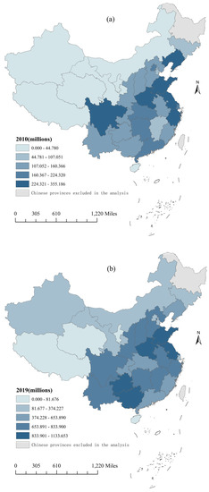
Figure 1.
Spatial distribution of domestic tourism demand. Note: Based on the data of domestic tourist arrivals in 2010 (a) and 2019 (b).
Domestic tourism demand is distributed significantly differently in time and space (lighter colors represent fewer domestic tourist arrivals, and darker colors represent more domestic tourist arrivals). Temporally, domestic tourism demand has grown dramatically over the decade, with total domestic tourist arrivals increasing from 4.5 billion in 2010 to 16.8 billion in 2019, with varying degrees of growth in all 30 provinces. Spatially, the eastern and central provinces are expanding more quickly (light blue becomes dark blue). Domestic tourists frequently opt to visit provinces with a higher degree of economic growth, easier access to transportation, and more robust infrastructure given China’s history and level of development.
Based on the fact that domestic tourism demand has obvious spatiotemporal differentiation characteristics, this study has the conditions for using the GWPR model for further research.
3.2. Model Evaluation
The GWR4.0 software was developed and programmed by Professor Tomoki Nakaya of the Department of Geography, Ritsumeikan University, Kyoto, Japan. It is a software tool for modeling varying relationships among variables by calibrating geographically weighted regression and geographically weighted generalized linear models with their semi-parametric variants. GWR4.0 allows one to fit a range of GWR models including conventional Gaussian models as well as extensions based on the generalized linear modeling framework. This includes geographically weighted Poisson and logistic regression models. So, this study uses GWR4.0 software to calculate statistical results. To determine the reasonableness of the model selection, the results of the OLS model and the GWPR model analysis were compared.
According to the results obtained by GWR4.0 software, we use three metrics, Akaike Information Criterion (AICc), Deviance, and Percent Deviance Explained (PDE) values, to compare the effects of the GWPR model with the OLS model. First, the AICc value is a metric for assessing the model’s accuracy and complexity; when the difference in AICc between two models is higher than 3, the model with the lower AICc is regarded as superior [76]. As shown in Table 1, the difference in AICc between the GWPR and OLS models in this research is much larger than 3, indicating that the GWPR model is a better model in this study. Second, the GWPR model’s deviance values are lower and its PDE values are more interpretable (higher) than the OLS model, indicating that the GWPR model has greater advantages over the OLS model over the 2010–2019 period.

Table 1.
Model evaluation between OLS regression and GWPR.
Table 2 displays the minimum, 1/4 quartile, median, 3/4 quartile, maximum, and global estimate results (OLS regression results) of each independent variable regression coefficient estimation result. As shown in Table 2, GWPR analysis results in 2010 showed that in the 30 provinces within the scope of this study, the maximum HSR coefficient was 2.585003, the minimum was −1.389550, the maximum aviation coefficient was 0.730374, and the minimum was −5.267311. In addition, the table also gave values for 1/4, median, and 3/4, while OLS regression could only obtain a global regression coefficient. The results in 2019 exhibit the same characteristics. Data results for the intermediate year 2015 can be found in Table A2 and Table A3 (Appendix A).
Table 2.
GWPR Results for the year 2010–2019.
Table 2 shows that each explanatory variable estimated by the GWPR model has a unique parameter value for domestic tourism demand in each province, revealing the geographical heterogeneity of the impact of various influencing variables on the explanatory variable across provinces. Furthermore, most of the quartiles have a considerable variation in parameter estimates, indicating that the impact of each explanatory variable is heterogeneous for most of the sample points in the region.
Therefore, the results of the GWPR model analysis are more accurate and detailed than the results of the OLS model study.
3.3. The Combined Effects of Transportation Infrastructure
Because this study focuses on the effects of transportation infrastructure factors on domestic tourism demand, only the results of the coefficients of transportation infrastructure variables in the regression findings of the GWPR model are presented (other coefficient results are available upon request by letter from the authors).
3.3.1. Overall Distribution of the Combined Effects
As illustrated in Table 3, based on the overall situation of the regression coefficient values, 23 out of the total 30 provinces in this study had positive values for both HSR and air impact coefficients in 2010. This suggests that both HSR and aviation have a positive impact on domestic tourism demand in the majority of China’s provinces, which is consistent with many research findings [29,30,77].
Table 3.
GWPR Results of HSR and Aviation.
In 2019, the impact coefficient of HSR was positive in all provinces. The impact coefficient values of HSR in all provinces have improved significantly compared to 2010, except in Shanxi and Gansu. Although Shanxi and Gansu’s influence has dwindled slightly, their overall impact remains high. In the same year, the situation for aviation is dire. Despite the fact that 20 provinces still have positive aviation coefficient values, indicating that the positive effect of aviation on domestic tourism demand remains, the majority of provinces (23/30) show a significant decrease in the value of the aviation coefficient when compared to 2010. The aviation coefficient values in ten provinces are either negative (Beijing, Jiangxi, Shandong, Hunan, Guangdong, Guizhou, Yunnan, and Xinjiang) or insignificant (Shanxi and Gansu). The ten provinces with a negative or insignificant aviation influence tend to have higher HSR coefficients over the same time period.
3.3.2. Spatiotemporal Distribution of the Combined Effects
The combined impact results of HSR and aviation in 2010 and 2019 are obtained based on the coefficient value results of HSR and aviation in 2010 and 2019 in Table 3. If the coefficient value is positive, it is determined to have a positive impact; if it is insignificant, it is determined to have an insignificant impact; if it is negative, it is determined to have a negative impact.
According to the spatial heterogeneity of the regression coefficient values, the combined impact of HSR and aviation on domestic tourism demand in 2010 presents four states, as illustrated in Figure 2. (1) “Negative and Negative”: Beijing, Tianjin, and Henan’s domestic tourism demand are negatively impacted by both HSR and aviation. Tourists flow to other provinces as HSR and aviation networks develop in other neighboring regions, resulting in a negative correlation in domestic tourism demand in these three provinces. (2) “Negative and Positive”: Hebei, Guangdong, Guizhou, and Ningxia are negatively affected by HSR and positively affected by aviation, indicating that domestic tourism demand in these provinces is still highly reliant on aviation. (3) “Positive and Negative”: in Shanxi, Anhui, Tibet, and Gansu, in contrast to the “negative and positive” type, the domestic tourism demand in these four provinces is highly dependent on HSR. (4) The remaining 19 provinces are all of the “Positive and Positive” type: provinces that benefit from both HSR and aviation, which account for the vast majority of China’s provinces.
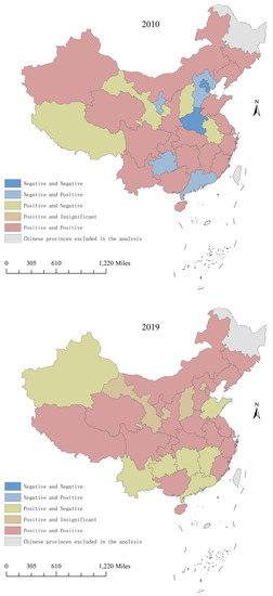
Figure 2.
Spatial distribution of the combined impact of HSR and aviation.
The year 2019 is a major change from 2010, with the combined impact of transportation infrastructure shown in three states. (1) “Positive and Insignificant”: HSR has a positive impact on Shanxi and Gansu, but aviation has no significant impact. HSR has had a significant impact on local tourism demand in the provinces since 2010. (2) “Positive and Negative”: HSR benefits Beijing, Jiangxi, Shandong, Hunan, Guangdong, Guizhou, Yunnan, and Xinjiang while aviation negatively affects them. In 2010, Beijing was “negative and negative”, while Guangdong and Guizhou were “negative and positive”. After ten years of development, HSR’s influence has turned positive. The status of Jiangxi, Shandong, Hunan, Yunnan, and Xinjiang has shifted from “positive and positive” to “positive and negative.” HSR has always had a positive impact in these five provinces, whereas aviation has turned negative. (3) The remaining 20 provinces are all of the “Positive and Positive” type: these types of regions still account for more than half of China’s provinces in 2019. Both HSR and aviation boost domestic tourism demand.
According to the trend results in Table 3, from 2010 to 2019, the evolution trend of the combined impact of HSR and aviation shows three states, as illustrated in Figure 3. (1) “Upward and Upward”: in Beijing, Tianjin, Anhui, Henan, and Tibet in 2019, the regression coefficients for the influence of HSR and aviation on domestic tourism demand are greater than in 2010, indicating that both are having a growing impact. (2) “Downward and Upward”: Shanxi and Gansu have a downward trend influenced by HSR and an upward trend influenced by aviation. The main reason is that HSR development in these two provinces is slow and limited to a single route. Due to the region’s rich tourism resources and strong attractions, a single HSR network is unable to meet the needs of tourists, resulting in increased reliance on aviation. (3) The remaining 23 regions are all “Upward and Downward”: these provinces all have a downward trend influenced by HSR and an upward trend influenced by aviation. This type of province is located in most regions of China, and it is distinguished by strong HSR development momentum and a shrinking aviation market.
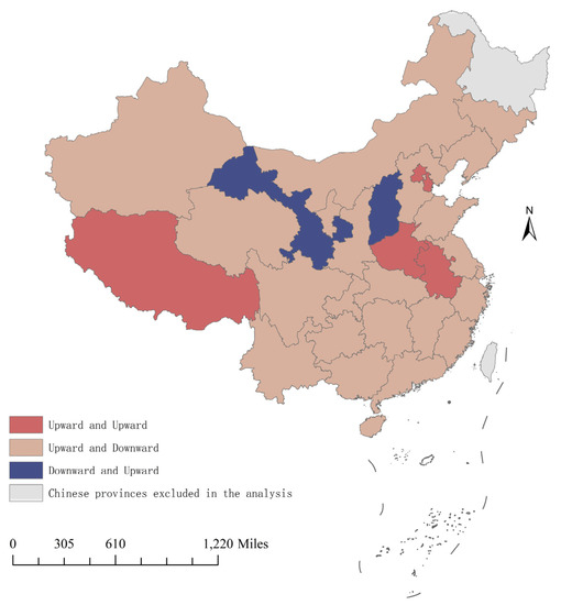
Figure 3.
Spatial distribution of the evolution trend of the combined impact.
Based on the combined effect status in 2019 (before the COVID-19 pandemic) and the evolution trend, the 30 provinces in this study are categorized into five types. The outcomes and spatial distribution are displayed in Figure 4 and Figure 5.
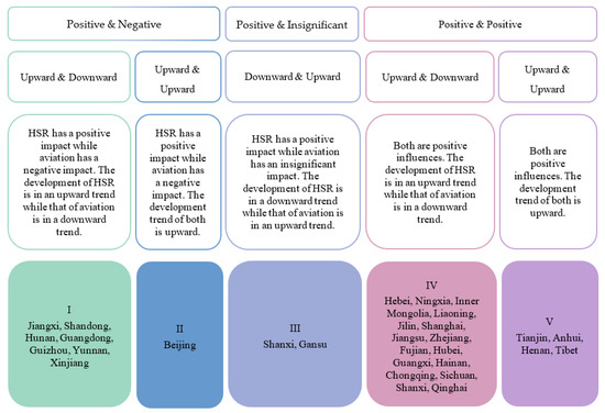
Figure 4.
Characteristics and types of different provinces. Note: This figure was drawn using Word and is based on the analysis results in Section 3.3.1 and Section 3.3.2.
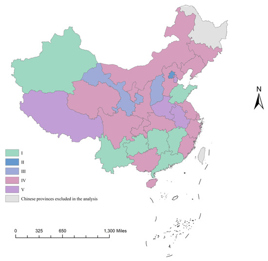
Figure 5.
Spatial distribution of the types of different provinces. Note: Based on the results of Figure 4.
According to the characteristics and types of combined impacts on transportation infrastructure, the following policy recommendations are proposed:
The provinces of Jiangxi, Shandong, Hunan, Guangdong, Guizhou, Yunnan, and Xinjiang are included in the same category and are distinguished by the positive influence of HSR and the upward trend, as well as the negative influence of aviation and the downward trend. In the post-epidemic era, these provinces should focus on changing aviation infrastructure development policies. Among possible strategies are expanding routes; deepening the product system; altering the ticket price strategy; improving the construction of the road network from the airport to scenic spots; and advocating the “seamless transfer” between aviation and other forms of transportation infrastructure.
Similarities can be discovered between Shanxi and Gansu, where aviation has an insignificant impact but an ascending tendency and HSR has a positive impact but a declining trend. The regional HSR network must be expanded in addition to other transportation infrastructure initiatives.
Beijing has the unique characteristics of HSR as a positive influence and aviation as a negative influence, but both of them have good development trends. We think that Beijing’s transportation system is now headed in the right direction. In the future, Beijing should further improve the road traffic construction from the airport to scenic spots, do a good job of “seamless transfer”, and improve the travel efficiency of tourists.
The combined effect of transportation infrastructure on domestic tourism demand was relatively strong in Hebei, Shanxi, Inner Mongolia, Liaoning, Jilin, Shanghai, Jiangsu, Zhejiang, Fujian, Hubei, Guangxi, Hainan, Chongqing, Sichuan, Qinghai, and Ningxia prior to the epidemic. Although there were divergent development trends, HSR’s influence was growing while aviation’s was declining. Future efforts should focus on strengthening aviation collaboration strategies and developing the “aviation and tourism integration” product system.
In Tianjin, Anhui, Henan, and Tibet, the combined impact of transportation infrastructure before the epidemic was relatively high, and the development trend was also good. In the post-epidemic era, they can continue to adopt the previous transportation infrastructure development policies and do a good job of scientific and steady development.
4. Discussions
4.1. Discussions
This paper uses the GWPR model to analyze the combined impact of HSR and aviation as the core explanatory variables on domestic tourism demand. Using 2010–2019 as a time series, this paper examines the spatial heterogeneity characteristics of the combined impact in 30 provinces in mainland China and makes recommendations for provincial development.
In general, some of the conclusions of this study have similarities with those of previous studies. We all believe that the relationship between HSR and aviation has both competitive and cooperative relationships in terms of the impact on domestic tourism demand [19,20,21,22,23,24,25,26,27,28].
We contribute to the current knowledge of tourism transportation and demand in two ways. First, we do not think the complementarity and substitution relationship between HSR and aviation is set in stone; instead, we look at the combined effect of the two on tourist arrivals in terms of temporal and spatial variability. This is a useful attempt to better understand the interaction between HSR and aviation as well as the influence on tourism, providing a broader perspective for the tourism industry in these provinces to cope with HSR’s rapid development. Clearly, there are numerous opportunities to further investigate this topic by examining their combined impact on other aspects of tourism demand (e.g., tourist consumption). Second, a few pieces of literature have focused on the combined influence of transportation modes on tourism development. Tian et al. (2022) estimated a spatial Durbin model to understand whether enhancements in road, air, railway, and HSR transport stimulated tourism growth in nearby regions and confirmed transport spillover [78]. Chen et al. (2022) developed a linear regression model to quantify and compare the influence of HSR and air transport on tourism and explore their relationships [79]. They both discussed the correlation between the comprehensive impact of transport infrastructure and tourism development through global models. Although some conclusions about regional heterogeneity have been proposed, the global models fundamentally treat geographic space as homogeneous. The local spatial regression model (GWPR) used in this paper has obvious advantages when analyzing spatial heterogeneity. The current research, by analyzing spatiotemporal panel data from the Chinese provinces, greatly extends the generalizability of the GWPR method to an important context.
4.2. Limitations
This paper does have certain flaws, which are mostly related to the limits of data collection. First, dummy variables are used in HSR and aviation. We still anticipate additional scientific and reasonable data sources, even if numerous studies have demonstrated the viability and scientificity of this approach [19,21,22,23,24,25,26,27,28]. Additionally, this article chooses the province as the research scale since the radiation effect of aviation is primarily centered in the province and there are not many airports in city-level locations. The city-level data have a natural advantage in analyzing the provincial administrative regions with significant spatial differences, and more meso- and micro-level studies can be considered in the future, even though the province-level data research has produced a number of desirable analysis results.
5. Conclusions
Taking provinces as the research scale and the period from 2010 to 2019 as the research interval, this paper uses the GWPR model to study the spatial and temporal differentiation of the combined impact of transportation infrastructure on domestic tourism demand and draws the following four conclusions:
First, spatiotemporal heterogeneity in the distribution of tourism demand can be observed, with the number of domestic tourists rising exponentially more in the eastern and central provinces than in the western provinces.
Second, the effects of transportation infrastructure on tourism have historically been overwhelmingly positive, with HSR’s positive effect expanding over the decade while air travel’s positive effect is contracting. Both HSR and aviation have a positive impact on domestic tourism demand in most provinces of China (23/30). However, the provinces with positive effects of HSR have increased from 23 in 2010 to 30 in 2019, while the provinces producing positive effects of aviation have decreased from 23 in 2010 to 20 in 2019.
Third, the combined effects of transportation infrastructure vary across space and time. The provinces showed four situations in 2010 and three situations in 2019. Additionally, the situation among provinces is also changing. For instance, the situation in eight provinces that were “positive and negative” in 2019 is all different from that of 2010.
Finally, the evolution of the effects exhibits spatial heterogeneity. The number of “upward and downward” regions ranked first, “upward and upward” regions ranked second, and “downward and upward” regions ranked the least, according to the evolution trend of HSR and aviation from 2010 to 2019.
Author Contributions
This study was carried out with the cooperation of P.S., P.Y. and B.N. Conceptualization, P.S. and P.Y.; methodology, P.S. and P.Y.; software, P.S. and B.N.; writing—original draft preparation, P.S.; writing—review and editing, P.Y.; funding acquisition, P.Y. All authors have read and agreed to the published version of the manuscript.
Funding
This research was funded by Fundamental Research Funds for the Central Universities, grant number 2021YJS076 and 2019JBWB002.
Institutional Review Board Statement
Not applicable.
Informed Consent Statement
Not applicable.
Data Availability Statement
The data used in this paper on domestic tourist arrivals, A-grade visitor attractions, and star-rated hotels are from the China Tourism Statistical Yearbook 2010–2019. Data for GDP per capita and transportation network density are from the China Statistical Yearbook 2010–2019. Airport data are from the official website of the Civil Aviation Administration of China. Data on HSR were manually gathered using the GAOTIE.cn web map. It should be noted that this study only includes HSR lines built after the Beijing–Tianjin Intercity Railway opened in 2008.
Conflicts of Interest
The authors declare no conflict of interest.
Appendix A
Table A1.
Summary of abbreviation.
Table A1.
Summary of abbreviation.
| Notation | Terms |
|---|---|
| GWPR | Geographically weighted Poisson regression |
| HSR | High-speed rail |
| COVID-19 | Coronavirus disease 2019 |
| GWR | Geographically weighted regression |
| DTD | Domestic tourism demand |
| UN | The United Nations |
| UNWTO | The World Tourism Organization |
| TI | Transportation infrastructure |
| GDP | Gross domestic product |
| OLS | Ordinary least squares |
| AICc | Akaike information criterion |
| PDE | Percent deviance explained |
Table A2.
GWPR Results for the year 2015.
Table A2.
GWPR Results for the year 2015.
| Variables | Min | Lwr Qu | Median | Upr Qu | Max | Global |
|---|---|---|---|---|---|---|
| intercept | 9.486451 | 9.882520 | 9.992392 | 10.092544 | 10.203027 | 10.178761 |
| HSR | 0.007920 | 0.187303 | 0.312568 | 0.454880 | 0.765968 | 0.222838 |
| aviation | −0.746067 | −0.074094 | 0.206052 | 0.269641 | 0.360710 | 0.050819 |
| attraction | −0.251569 | −0.063836 | 0.104214 | 0.329831 | 0.581489 | 0.052145 |
| GDP | −1.339842 | −0.630809 | −0.311151 | 0.110518 | 0.228510 | −0.281555 |
| accommodation | −0.101985 | 0.173663 | 0.395279 | 0.532336 | 0.904525 | 0.298826 |
| local transportation | −0.235290 | 0.163485 | 0.409166 | 0.556697 | 0.799853 | 0.376908 |
Table A3.
GWPR Results of HSR and Aviation in 2015.
Table A3.
GWPR Results of HSR and Aviation in 2015.
| Region | 2015 | |
|---|---|---|
| HSR | Aviation | |
| Beijing | 0.155195 | −0.71221 |
| Tianjin | 0.15029 | 0.36071 |
| Hebei | 0.306179 | −0.746067 |
| Shanxi | 0.134892 | −0.258413 |
| Inner Mongolia | 0.229975 | 0.289284 |
| Liaoning | 0.174055 | 0.250666 |
| Jilin | 0.139715 | 0.051086 |
| Shanghai | 0.292801 | 0.159085 |
| Jiangsu | 0.584585 | 0.077409 |
| Zhejiang | 0.4503 | 0.150594 |
| Anhui | 0.505684 | −0.167121 |
| Fujian | 0.353944 | 0.206052 |
| Jiangxi | 0.105885 | −0.074094 |
| Shandong | 0.304805 | 0.041983 |
| Henan | 0.765968 | −0.086115 |
| Hubei | 0.325275 | 0.230633 |
| Hunan | 0.226397 | −0.000049 |
| Guangdong | 0.606156 | −0.005029 |
| Guangxi | 0.45488 | 0.231918 |
| Hainan | 0.43241 | 0.279292 |
| Chongqing | 0.539732 | 0.207956 |
| Sichuan | 0.38765 | 0.271292 |
| Guizhou | 0.438284 | 0.210974 |
| Yunnan | 0.617226 | 0.250851 |
| Tibet | 0.43042 | 0.279754 |
| Shaanxi | 0.47842 | 0.295907 |
| Gansu | 0.312568 | 0.269641 |
| Qinghai | 0.187303 | 0.231695 |
| Ningxia | 0.31171 | −0.248688 |
| Xinjiang | 0.00792 | −0.137388 |
References
- Abeyratne, R.I.R. Air Transport Tax and its Consequences on Tourisms. Ann. Tour. Res. 1993, 20, 450–460. [Google Scholar] [CrossRef]
- Chew, J. Transport and Tourism in the Year 2000. Tour. Manag. 1987, 8, 83–85. [Google Scholar] [CrossRef]
- Campa, J.L.; López-Lambas, M.E.; Guirao, B. High Speed Rail Effects on Tourism: Spanish Empirical Evidence Derived From China’s Modelling Experience. J. Transp. Geogr. 2016, 57, 44–54. [Google Scholar] [CrossRef] [PubMed]
- Kanwal, S.; Rasheed, M.I.; Pitafi, A.H.; Pitafi, A.; Ren, M. Road and Transport Infrastructure Development and Community Support for Tourism: The Role of Perceived Benefits, and Community Satisfaction. Tour. Manag. 2020, 77, 104014. [Google Scholar] [CrossRef]
- Martin, C.A.; Witt, S.F. Substitute Prices in Models of Tourism Demand. Ann. Tour. Res. 1988, 15, 255–268. [Google Scholar] [CrossRef]
- Yu, D.; Murakami, D.; Zhang, Y.; Wu, X.; Li, D.; Wang, X.; Li, G. Investigating High-Speed Rail Construction’s Support to County Level Regional Development in China: An Eigenvector Based Spatial Filtering Panel Data Analysis. Transp. Res. Part B. 2020, 133, 21–37. [Google Scholar] [CrossRef]
- Chen, A.; Li, Y.; Ye, K.; Nie, T.; Liu, R. Does Transport Infrastructure Inequality Matter for Economic Growth? Evidence from China. Land 2021, 10, 874. [Google Scholar] [CrossRef]
- Khadaroo, J.; Seetanah, B. Transport Infrastructure and Tourism Development. Ann. Tour. Res. 2007, 34, 1021–1032. [Google Scholar] [CrossRef]
- Speakman, C. Tourism and Transport: Future Prospects. Tour. Hos. Plan. Dev. 2005, 2, 129–135. [Google Scholar] [CrossRef]
- Prideaux, B. The Role of the Transport System in Destination Development. Tour. Manag. 2000, 21, 53–63. [Google Scholar] [CrossRef]
- de Oliveira Santos, G.E.; Perinotto, A.R.C.; Silveira, C.E.; Silveira, J.M.; Lobo, H.A.S.; Minasse, M.H.S.G.G.; Travassos, L.E.P. Demanda turística por destinos com severas limitações de acesso: Casos brasileiros. Pasos Rev. Turismo Patrim. Cult. 2017, 15, 519–531. [Google Scholar] [CrossRef]
- Wendt, J.A.; Grama, V.; Ilieş, G.; Mikhaylov, A.S.; Borza, S.G.; Herman, G.V.; Bógdał-Brzezińska, A. Transport Infrastructure and Political Factors as Determinants of Tourism Development in the Cross-Border Region of Bihor and Maramureş. A Comparative Analysis. Sustainability 2021, 13, 5385. [Google Scholar] [CrossRef]
- Albalate, D.; Fageda, X. High Speed Rail and Tourism: Empirical Evidence from Spain. Transp. Res. Part A 2016, 85, 174–185. [Google Scholar] [CrossRef]
- Takebayashi, M. Workability of a Multiple-Gateway Airport System with a High-Speed Rail Network. Transp. Policy 2021, 107, 61–71. [Google Scholar] [CrossRef]
- Li, L.S.Z.; Yang, F.X.; Cui, C. High-Speed Rail and Tourism in China: An Urban Agglomeration Perspective. Int. J. Tour. Res. 2019, 21, 45–60. [Google Scholar] [CrossRef]
- Liu, Y.; Shi, J. How Inter-City High-Speed Rail Influences Tourism Arrivals: Evidence from Social Media Check-in Data. Curr. Issues Tour. 2019, 22, 1025–1042. [Google Scholar] [CrossRef]
- Spasojevic, B.; Lohmann, G.; Scott, N. Air Transport and Tourism—A Systematic Literature Review (2000–2014). Curr. Issues Tour. 2018, 21, 975–997. [Google Scholar] [CrossRef]
- Wang, K.; Tsui, W.H.K.; Li, L.; Lei, Z.; Fu, X. Entry Pattern of Low-Cost Carriers in New Zealand—The Impact of Domestic and Trans-Tasman Market Factors. Transp. Policy 2020, 93, 36–45. [Google Scholar] [CrossRef]
- Yang, Z.; Li, T. Does High-Speed Rail Boost Urban Tourism Economy in China? Curr. Issues Tour. 2020, 23, 1973–1989. [Google Scholar] [CrossRef]
- Yang, Y.; Li, D.; Li, X.R. Public Transport Connectivity and Intercity Tourist Flows. J. Travel Res. 2019, 58, 25–41. [Google Scholar] [CrossRef]
- Avogadro, N.; Cattaneo, M.; Paleari, S.; Redondi, R. Replacing Short-Medium Haul Intra-European Flights with High-Speed Rail: Impact on Co2 Emissions and Regional Accessibility. Transp. Policy 2021, 114, 25–39. [Google Scholar] [CrossRef]
- Chai, J.; Zhou, Y.; Zhou, X.; Wang, S.; Zhang, Z.G.; Liu, Z. Analysis on Shock Effect of China’s High-Speed Railway on Aviation Transport. Transp. Res. Part A 2018, 108, 35–44. [Google Scholar] [CrossRef]
- Chen, Z.; Wang, Z.; Jiang, H. Analyzing the Heterogeneous Impacts of High-Speed Rail Entry on Air Travel in China: A Hierarchical Panel Regression Approach. Transp. Res. Part A 2019, 127, 86–98. [Google Scholar] [CrossRef]
- Dobruszkes, F. High-Speed Rail and Air Transport Competition in Western Europe: A Supply-Oriented Perspective. Transp. Policy 2011, 18, 870–879. [Google Scholar] [CrossRef]
- Mizutani, J.; Sakai, H. Which is a Stronger Competitor, High Speed Rail, or Low Cost Carrier, to Full Service Carrier?—Effects of Hsr Network Extension and Lcc Entry on Fsc’s Airfare in Japan. J. Air Transp. Manag. 2021, 90, 101965. [Google Scholar] [CrossRef]
- Su, M.; Luan, W.; Fu, X.; Yang, Z.; Zhang, R. The Competition Effects of Low-Cost Carriers and High-Speed Rail on the Chinese Aviation Market. Transp. Policy 2020, 95, 37–46. [Google Scholar] [CrossRef]
- Yu, K.; Strauss, J.; Liu, S.; Li, H.; Kuang, X.; Wu, J. Effects of Railway Speed on Aviation Demand and Co2 Emissions in China. Transp. Res. Part D 2021, 94, 102772. [Google Scholar] [CrossRef]
- Albalate, D.; Bel, G.; Fageda, X. Competition and Cooperation between High-Speed Rail and Air Transportation Services in Europe. J. Transp. Geogr. 2015, 42, 166–174. [Google Scholar] [CrossRef]
- Wan, Y.; Ha, H.; Yoshida, Y.; Zhang, A. Airlines’ Reaction to High-Speed Rail Entries: Empirical Study of the Northeast Asian Market. Transp. Part Res. A 2016, 94, 532–557. [Google Scholar] [CrossRef]
- Zhang, F.; Graham, D.J.; Wong, M.S.C. Quantifying the Substitutability and Complementarity between High-Speed Rail and Air Transport. Transp. Res. Part A 2018, 118, 191–215. [Google Scholar] [CrossRef]
- Liu, H.; Liu, W.; Wang, Y. A Study on the Influencing Factors of Tourism Demand from Mainland China to Hong Kong. J. Hosp. Tour. Res. 2021, 45, 171–191. [Google Scholar] [CrossRef]
- Carneiro, J.; Allis, T. How Does Tourism Move During the COVID-19 Pandemic? Braz. J. Tour. Res. 2021, 15, 1–23. [Google Scholar]
- Chen, Z. Measuring the Regional Economic Impacts of High-Speed Rail Using a Dynamic Scge Model: The Case of China. Eur. Plan. Stud. 2019, 27, 483–512. [Google Scholar] [CrossRef]
- Chen, Z.; Li, Y.; Wang, P. Transportation Accessibility and Regional Growth in the Greater Bay Area of China. Transp. Res. Part D 2020, 86, 102453. [Google Scholar] [CrossRef]
- Chen, Z.; Zhou, Y.; Haynes, K.E. Change in Land Use Structure in Urban China: Does the Development of High-Speed Rail Make a Difference. Land Use Pol. 2021, 111, 104962. [Google Scholar] [CrossRef]
- Losada, N.; Alén, E.; Cotos-Yáñez, T.R.; Domínguez, T. Spatial Heterogeneity in Spain for Senior Travel Behavior. Tour. Manag. 2019, 70, 444–452. [Google Scholar] [CrossRef]
- Wang, J.; Huang, J.; Jing, Y. Competition between High-Speed Trains and Air Travel in China: From a Spatial to Spatiotemporal Perspective. Transp. Res. Part A 2020, 133, 62–78. [Google Scholar] [CrossRef]
- Yang, Y.; Fik, T. Spatial Effects in Regional Tourism Growth. Ann. Tour. Res. 2014, 46, 144–162. [Google Scholar] [CrossRef]
- Zhou, B.; Wen, Z.; Yang, Y. Agglomerating or Dispersing? Spatial Effects of High-Speed Trains on Regional Tourism Economies. Tour. Manag. 2021, 87, 104392. [Google Scholar] [CrossRef]
- He, Y.; Sherbinin, A.D.; Shi, G.; Xia, H. The Economic Spatial Structure Evolution of Urban Agglomeration Under the Impact of High-Speed Rail Construction: Is there a Difference between Developed and Developing Regions? Land 2022, 11, 1551. [Google Scholar] [CrossRef]
- Niu, F.; Wang, F. Economic Spatial Structure in China: Evidence from Railway Transport Network. Land 2022, 11, 61. [Google Scholar] [CrossRef]
- Zhao, S.; Zhao, K.; Yan, Y.; Zhu, K.; Guan, C. Spatio-Temporal Evolution Characteristics and Influencing Factors of Urban Service-Industry Land in China. Land 2022, 11, 13. [Google Scholar] [CrossRef]
- Tobler, W.R. A Computer Movie Simulating Urban Growth in the Detroit Region. Econ. Geogr. 1970, 46, 234. [Google Scholar] [CrossRef]
- Brunsdon, C.; Fotheringham, A.S.; Charlton, M.E. Geographically Weighted Regression: A Method for Exploring Spatial Nonstationarity. Geogr. Anal. 1996, 28, 281–298. [Google Scholar] [CrossRef]
- Bai, X.; Zhai, W.; Steiner, R.L.; He, Z. Exploring Extreme Commuting and its Relationship to Land Use and Socioeconomics in the Central Puget Sound. Transp. Res. Part D 2020, 88, 102574. [Google Scholar] [CrossRef]
- Tang, J.; Gao, F.; Han, C.; Cen, X.; Li, Z. Uncovering the Spatially Heterogeneous Effects of Shared Mobility on Public Transit and Taxi. J. Transp. Geogr. 2021, 95, 103134. [Google Scholar] [CrossRef]
- Wang, C.; Chen, N. A Multi-Objective Optimization Approach to Balancing Economic Efficiency and Equity in Accessibility to Multi-Use Paths. Transportation 2021, 48, 1967–1986. [Google Scholar] [CrossRef]
- Nakaya, T.; Fotheringham, A.S.; Brunsdon, C.; Charlton, M. Geographically Weighted Poisson Regression for Disease Association Mapping. Stat. Med. 2005, 24, 2695–2717. [Google Scholar] [CrossRef] [PubMed]
- Pagliara, F.; Mauriello, F. Modelling the Impact of High Speed Rail on Tourists with Geographically Weighted Poisson Regression. Transp. Res. Part A 2020, 132, 780–790. [Google Scholar] [CrossRef]
- Gardiner, S.; Grace, D.; King, C. The Generation Effect: The Future of Domestic Tourism in Australia. J. Travel Res. 2014, 53, 705–720. [Google Scholar] [CrossRef]
- Otero-Giráldez, M.S.; Álvarez-Díaz, M.; González-Gómez, M. Estimating the Long-Run Effects of Socioeconomic and Meteorological Factors on the Domestic Tourism Demand for Galicia (Spain). Tour. Manag. 2012, 33, 1301–1308. [Google Scholar] [CrossRef]
- Seddighi, H.R.; Shearing, D.F. The Demand for Tourism in North East England with Special Reference to Northumbria: An Empirical Analysis. Tour. Manag. 1997, 18, 499–511. [Google Scholar] [CrossRef]
- Barbhuiya, M.R.; Chatterjee, D. Vulnerability and Resilience of the Tourism Sector in India: Effects of Natural Disasters and Internal Conflict. Tour. Manag. Perspect. 2020, 33, 100616. [Google Scholar] [CrossRef]
- Karamelikli, H.; Khan, A.A.; Karimi, M.S. Is Terrorism a Real Threat to Tourism Development? Analysis of Inbound and Domestic Tourist Arrivals in Turkey. Curr. Issues Tour. 2020, 23, 2165–2181. [Google Scholar] [CrossRef]
- Volo, S. Research Note: Seasonality in Sicilian Tourism Demand—An Exploratory Study. Tour. Econ. 2010, 16, 1073–1080. [Google Scholar] [CrossRef]
- Wang, L.; Chen, M. Nonlinear Impact of Air Quality on Tourist Arrivals: New Proposal and Evidence. J. Travel Res. 2021, 60, 434–445. [Google Scholar] [CrossRef]
- Albalate, D.; Campos, J.; Jiménez, J.L. Tourism and High Speed Rail in Spain: Does the Ave Increase Local Visitors? Ann. Tour. Res. 2017, 65, 71–82. [Google Scholar] [CrossRef]
- Chen, Z.; Haynes, K.E. Impact of High Speed Rail on Housing Values: An Observation from the Beijing–Shanghai Line. J. Transp. Geogr. 2015, 43, 91–100. [Google Scholar] [CrossRef]
- Donaldson, D. Railroads of the Raj: Estimating the Impact of Transportation Infrastructure. Am. Econ. Rev. 2018, 108, 899–934. [Google Scholar] [CrossRef]
- Gao, Y.; Su, W.; Wang, K. Does High-Speed Rail Boost Tourism Growth? New Evidence from China. Tour. Manag. 2019, 72, 220–231. [Google Scholar] [CrossRef]
- Shao, S.; Tian, Z.; Yang, L. High Speed Rail and Urban Service Industry Agglomeration: Evidence from China’s Yangtze River Delta Region. J. Transp. Geogr. 2017, 64, 174–183. [Google Scholar] [CrossRef]
- Massidda, C.; Etzo, I. The Determinants of Italian Domestic Tourism: A Panel Data Analysis. Tour. Manag. 2012, 33, 603–610. [Google Scholar] [CrossRef]
- Wang, T.; Wu, P.; Ge, Q.; Ning, Z. Ticket Prices and Revenue Levels of Tourist Attractions in China: Spatial Differentiation between Prefectural Units. Tour. Manag. 2021, 83, 104214. [Google Scholar] [CrossRef]
- Wang, L.; Tian, B.; Filimonau, V.; Ning, Z.; Yang, X. The Impact of the Covid-19 Pandemic on Revenues of Visitor Attractions: An Exploratory and Preliminary Study in China. Tour. Econ. 2022, 28, 153–174. [Google Scholar] [CrossRef]
- Valjarević, A.; Vukoičić, D.; Valjarević, D. Evaluation of the Tourist Potential and Natural Attractivity of the Lukovska Spa. Tour. Manag. Perspect. 2017, 22, 7–16. [Google Scholar] [CrossRef]
- Ruan, W.; Zhang, S. Can Tourism Information Flow Enhance Regional Tourism Economic Linkages? J. Hosp. Tour. Manag. 2021, 49, 614–623. [Google Scholar] [CrossRef]
- Manes, E.; Tchetchik, A. The Role of Electronic Word of Mouth in Reducing Information Asymmetry: An Empirical Investigation of Online Hotel Booking. J. Bus. Res. 2018, 85, 185–196. [Google Scholar] [CrossRef]
- Razavi, R.; Israeli, A.A. Determinants of Online Hotel Room Prices: Comparing Supply-Side and Demand-Side Decisions. Int. J. Contemp. Hosp. Manag. 2019, 31, 2149–2168. [Google Scholar] [CrossRef]
- Walheer, B.; Zhang, L. Profit Luenberger and Malmquist-Luenberger Indexes for Multi-Activity Decision-Making Units: The Case of the Star-Rated Hotel Industry in China. Tour. Manag. 2018, 69, 1–11. [Google Scholar] [CrossRef]
- Tang, X.; Wang, D.; Sun, Y.; Chen, M.; Waygood, E.O.D. Choice Behavior of Tourism Destination and Travel Mode: A Case Study of Local Residents in Hangzhou, China. J. Transp. Geogr. 2020, 89, 102895. [Google Scholar] [CrossRef]
- Wang, J.; Liang, M. Characteristics of Visitor Expenditure in Macao and their Impact on its Economic Growth. Tour. Econ. 2018, 24, 218–233. [Google Scholar] [CrossRef]
- Hughes, R.; MacKenzie, D. Transportation Network Company Wait Times in Greater Seattle, and Relationship to Socioeconomic Indicators. J. Transp. Geogr. 2016, 56, 36–44. [Google Scholar] [CrossRef]
- Wang, S.; Noland, R.B. Variation in Ride-Hailing Trips in Chengdu, China. Transp. Res. Part D 2021, 90, 102596. [Google Scholar] [CrossRef]
- Bound, J.; Jaeger, D.A.; Baker, R.M. Problems with Instrumental Variables Estimation When the Correlation between the Instruments and the Endogeneous Explanatory Variable is Weak. J. Am. Stat. Assoc. 1995, 90, 443. [Google Scholar] [CrossRef]
- Wooldridge, J.M. Econometric Analysis of Cross-Section and Panel Data, 2nd ed.; The MIT Press: London, UK, 2010; pp. 469–522, 723–769. [Google Scholar]
- Brown, S.; Versace, V.L.; Laurenson, L.; Ierodiaconou, D.; Fawcett, J.; Salzman, S. Assessment of Spatiotemporal Varying Relationships Between Rainfall, Land Cover and Surface Water Area Using Geographically Weighted Regression. Environ. Model. Assess. 2011, 17, 241–254. [Google Scholar] [CrossRef]
- Xia, W.; Zhang, A. High-Speed Rail and Air Transport Competition and Cooperation: A Vertical Differentiation Approach. Transp. Res. Part B 2016, 94, 456–481. [Google Scholar] [CrossRef]
- Chen, J.; Yan, N.; Lin, S.; Chen, S. Comparative Analysis of the Influence of Transport Modes on Tourism: High-Speed Rail or Air? City-Level Evidence from China. Transport. Res. Rec. 2022, 862748296. [Google Scholar] [CrossRef]
- Tian, F.; Yang, Y.; Jiang, L. Spatial Spillover of Transport Improvement on Tourism Growth. Tour. Econ. 2022, 28, 1416–1432. [Google Scholar] [CrossRef]


Disclaimer/Publisher’s Note: The statements, opinions and data contained in all publications are solely those of the individual author(s) and contributor(s) and not of MDPI and/or the editor(s). MDPI and/or the editor(s) disclaim responsibility for any injury to people or property resulting from any ideas, methods, instructions or products referred to in the content. |
© 2023 by the authors. Licensee MDPI, Basel, Switzerland. This article is an open access article distributed under the terms and conditions of the Creative Commons Attribution (CC BY) license (https://creativecommons.org/licenses/by/4.0/).