Abstract
As a proxy for human activity, per capita urban land has great significance for urban planning. We still lack a comprehensive understanding of per capita urban land from the perspective of urban–rural gradients. Thus, based on the concentric buffering method and the dynamic-time-warp clustering method, this research analyzes the urban–rural gradient of the per capita urban land of 345 cities in China in 2000, 2010, and 2016. We find that the per capita urban land in China grew from 110.2 m2/person in 2000 to 118.9 m2/person, increasing by 7.9%. The urban–rural gradient of the per capita urban land can be classified into six types: (1) large city with a mono peak; (2) large city with a fluctuating increase; (3) medium city with a mono peak; (4) medium city with a declining trend; (5) small city with a mono peak, and (6) small city with a declining trend. In addition, most cities shifted from a mono-peak type to a declining type, which suggested that the low-density, sprawling development was intensifying. The dynamic-time-warp clustering method used in this research can effectively compare trends of the urban–rural gradient of per capita urban land across cities, which can be applied to the analysis of the urban–rural gradient of air pollution, urban green space, and urban heat islands.
1. Introduction
Per capita urban land is defined as the total area of urban land in a city divided by its population, and is an important proxy for urban development and its stress on the environment [1,2,3]. It is also an important factor considered in urban planning and land-use planning [4], and is a crucial variable used to project urban land dynamics in the future [5]. In the past thirty years, China has experienced rapid urbanization [6]. The urbanization ratio (i.e., proportion of urban population relative to total population) in China soared from 17.9% in 1978 to 56.1% in 2015 [7]. Meanwhile, China also experienced the largest share of urban expansion, accounting for 20.8% of the global increase [8]. From 2000 to 2020, urban land areas in China were estimated to expand by 7.33 × 10⁴ km2 [9]. With the rapid urbanization in China, the per capita urban land area is also changing rapidly [10]. Such changes have manifested in a problematic way; for instance, low-density and low-efficiency urban land expansion to rural areas [11,12], the occupation of croplands [13], sporadically illegal constructions [14], and the repeated overshooting of per capita urban land in terms of the national standard. Meanwhile, the urban–rural gradient in per capita urban land is commonly accompanied by an urban–rural gradient in air pollution [15,16], urban heat island effect [17], and social inequality [18]. Thus, analyzing the spatiotemporal changes in per capita urban land from the perspective of urban–rural gradients is fundamental for future urban planning and urban sustainable development.
Researchers have made some progress in analyzing the per capita urban land in China and around the world [19]. For example, Fang et al. [20] found that the per capita urban land increased by 2.8 times in China by using the census data. Liu et al. [21] analyzed urban expansion since the economic reform and opening-up in China using remote sensing data and found that economic development was the major driver of the increase in per capita urban land in China. Meanwhile, some scholars have focused on applying the per capita urban land in planning. For instance, Xu et al. [22] compared historical per capita urban land in 1995 and its estimated value in 2010 and argued that China should loosen the limit on the per capita urban land of large cities. Zhou et al. [23] believed that a reliable measurement of per capita urban land is strongly needed for urban planning in China. In terms of the spatial scales, most recent studies have focused on the investigations between China and foreign countries or within several regions in China. For example, Tan et al. [4] compared the per capita urban land between China and other countries. Tan et al. [24] compared the per capita urban land in China at the national scale. Zhou et al. [25] examined per capita urban land in Hubei Province; and Tan et al. [24] investigated the changes in per capita urban land in the Beijing–Tianjin–Hebei region.
However, there are few studies on the per capita urban land in China among cities from the perspective of the urban–rural gradient. Previous studies have investigated the changing trend of per capita urban land nationwide [20,22]. However, most of these studies were based on census data, which cannot delineate the urban–rural gradient of per capita urban land in a spatially explicit way. In fact, the per capita urban land has shown an urban–rural gradient because urban population and urban land area also exhibit an urban–rural gradient. Such a gradient has been portrayed by an S-shaped function of urban land density among 28 cities in China [26] and a declining urban population density model in Beijing by Chen et al. [27]. However, existing methods may not be suitable for comparing a large number of cities with varying sizes, especially those which do not follow an S-shape function. In terms of the comparison among cities, most studies were limited to a single city or an urban agglomeration. For example, Wang et al. [28] analyzed the urban land per capita of 55 major mountain cities in China. Ha et al. [29] took the urban land per capita as an indicator to evaluate land intensification in Urumqi. In a summary, a comparison among cities in China from an urban–rural gradient is still lacking.
The objective of this study is to explore the rural–urban gradient of the urban land per capita among China’s cities. We have two specific research questions: (1) How did the per capita urban land in Chinese cities change from 2000 to 2016? (2) Are there patterns of urban land per capita along the urban–rural gradient? First, we used the concentric buffering method to quantify the per capita urban land in each city. Next, we divided these cities into six types based on the DTW clustering method. After that, we investigated the spatiotemporal changes in the gradient of the per capita urban land in China in 2000, 2010, and 2016. Finally, we discussed the implications of the change on the urban–rural gradient of the per capita urban land for National Terrestrial Land Planning.
2. Materials and Methods
2.1. Study Area
This study analyzed the spatial and temporal dynamics of the urban land per capita in China at the city scale. This paper focused on 345 cities, including 291 prefecture-level cities, 40 provincial cities, and 4 municipalities directly under the Central Government of China (Figure 1). For the regional comparison, we referred to an existing study [30] and divided the study area into eight regions: Eastern Coastal China (ECC), the Middle Reaches of the Yellow River (MRYLR), the Middle Reaches of the Yangtze River (MRYTR), Northeast China (NEC), Northwest China (NWC), Northern Coastal China (NCC), Southern Coastal China (SCC), and Southwest China (SWC).
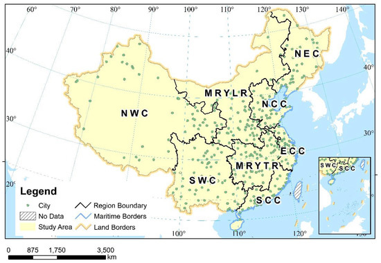
Figure 1.
Study Area. Note: Eastern Coastal China (ECC), Middle Reaches of the Yellow River (MRYLR), Middle Reaches of the Yangtze River (MRYTR), Northeast China (NEC), Northwest China (NWC), Northern Coastal China (NCC), Southern Coastal China (SCC), and Southwest China (SWC).
2.2. Data
This study mainly used urban land and population data. First, we used urban land data with a resolution of 1 km in 2000, 2010, and 2016 [8]. Here, referring to the hierarchical definitions of urban land [31], we defined urban land as the land dominated (having more than 50% in cover) by non-vegetated, human-constructed elements such as roads, buildings, runways, and industrial facilities. This set of data is based on a fully convolutional network to retrieve global urban land and its dynamics, with an overall accuracy of 90.9% and an average Kappa coefficient of 0.5. This dataset has been widely used for global analysis [4,13]. Second, we used the 1 km resolution Worldpop dataset for the population (https://www.worldpop.org/, accessed on 20 September 2020). This dataset was widely used in analyzing population distribution in China and worldwide [11,32]. To match the urban land data, we used the three periods of 2000, 2010, and 2016 for the population data. Finally, the location of the municipal government was used as the center of the city. Although the location of the municipal government may not be urban center, it will not affect the main objective of this study (i.e., developing a method to depict the urban-rural gradient of per capita urban land).
2.3. Methods
We examined the dynamics of the urban land per capita using the following four steps. First, we calculated the mean value of the urban land per capita at the city scale. Second, we measured the urban–rural gradient of the urban land per capita by using the concentric buffering method. Third, we classified the cities into several types based on the size of the city and the urban–rural gradient of the urban land per capita using the DTW clustering method (Figure 2). Finally, we analyzed the spatiotemporal dynamics of the urban land per capita from 2000 to 2016 among cities in China. The concentric buffers were operated using the “Buffer” and “Zonal Stats” modules of ArcGIS, and the DTW clustering method was achieved using the Python scipy library (https://scipy.org/ accessed on 30 December 2020).
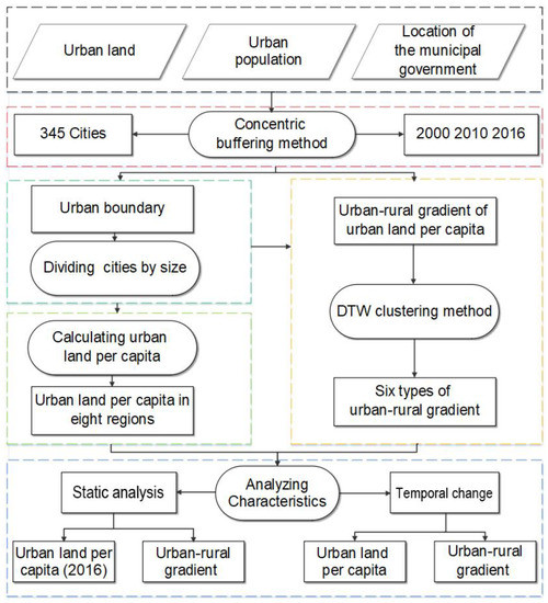
Figure 2.
Flow Chart of this study.
2.3.1. Calculating Urban Land per Capita
- (1)
- Determining the maximum distance of buffers
First, considering the heterogeneity of socioeconomic conditions among cities, we set the location of the local municipal government as the center of the buffering circle. Second, considering that the minimum spatial resolution of the data was 1 km, we set each buffer at a distance of 1 km. For the maximum distance of buffers, we assumed that the largest buffer could cover all spatially contiguous patches of urban land as well as some leapfrogging patches. Therefore, the maximum distance of buffers for each city was the distance in which there was no urban land outside this distance for at least five buffering circles (i.e., 5 km). The decision to use 5 km for the threshold was due to the fact that many leapfrogging centers (such as university towns and industrial parks) are 5–10 km away from the existing urban periphery. Meanwhile, to avoid overlapping maximum distances of buffers between two large cities, we set 50 km as the upper limit for the maximum distances for buffers of a city. This is because the average distance of the 345 cities is approximately 89 km, half of which is close to 50 km. Therefore, we used 50 km as the maximum distance for buffers.
Among the 345 cities in this study, the range of the maximum distances of buffers varied greatly. To avoid the incomparability of urban–rural gradients of the urban land per capita in cities with differing sizes, we divided the 345 cities into three categories according to the maximum distance of their buffers. Specifically, based on the distribution between the maximum distance of buffers and the number of cities, and on the premise that the number of the three types of cities should be similar, cities with a maximum distance of buffers less than 10 km were defined as small cities, including 98 in 2000, 82 in 2010 and 75 in 2016. Cities with a maximum distance of buffers between 10 and 25 km were defined as medium-sized cities: 97 in 2000, 111 in 2010, and 115 cities in 2016. Cities with a maximum distance of buffers larger than 25 km were classified as large cities, with 91 cities in 2000, 108 in 2010, and 112 in 2016. In addition, we excluded the cities with a maximum distance of buffers less than 5 km (51 cities in 2020, 36 cities in 2010, and 35 cities in 2016) because the distance was too short to analyze the urban–rural gradient.
- (2)
- Calculating the urban land per capita
We calculated the urban land per capita at the city scale. Specifically, we counted the urban land per capita by dividing the total amount of urban land by population within the urban boundary:
where D is the urban land per capita of a city; S is the total amount of urban land within the maximum distance of buffers; and P is the total amount of population within the maximum distance of buffers.
2.3.2. Analyzing the Urban–Rural Gradient of Urban Land per Capita
- (1)
- Quantifying the urban–rural gradient of urban land per capita
We used the circular buffering method to quantify the urban–rural gradient of the urban land per capita. This method makes a series of equidistant buffer zones outward from the city center to describe the changes in the examined features along the urban–rural gradient; a common method studying urban features. For example, Seto et al. [33] compared the urban–rural gradient of landscape metrics of land use in four Chinese cities. Jiao [26] observed an “inverted S-shape law” of urban land density outward from the urban center by using the circular buffering method. Here, we calculated the urban land per capita of each buffering circle to form an urban–rural curve of the urban land per capita for each city in the selected years:
where Dring is the urban land per capita of the buffering zone, Sbuilt-up is the total urban land area of each buffering ring, and Pring is the total population in the buffering zone.
- (2)
- Classifying the types of urban–rural gradients of the urban land per capita
We classified the 345 cities in 2000, 2010, and 2016 into several types based on their urban–rural gradients of the urban land per capita. Regarding the clustering method, hierarchical clustering was used to ensure the maximum variance between groups and the minimum variance within groups. Based on the characteristics of the urban–rural gradient data of per capita urban land, the DTW method was used to calculate the distance between groups instead of the traditional clustering method.
The DTW method is one of the clustering methods developed for time series data. This method mainly measures the similarity or distance between time series based on dynamic time warping [34]. The traditional clustering method usually only calculates the distance of corresponding points between samples but does not consider the overall shape similarity of time series data. Thus, traditional methods may divide two time-series data with a similar shape but a large absolute distance into two categories. For example, Line 1 in Figure 3a is similar to Line 2 in overall shape, but the two lines differ greatly using the traditional Euclidean distance (the Euclidean distance is 17.11). However, according to the DTW algorithm, points at similar positions on the two curves can be stretched and deformed (Figure 3b), and then the distance between curves can be calculated (the distance after the DTW is 7.00). In other words, the DTW algorithm is more suitable for estimating the similarity of change trends. Here, we mainly focused on the trend of urban land per capita along the urban–rural gradient rather than the absolute value between cities. Therefore, we chose the DTW method for clustering. We also compared the DTW method and traditional method in the Discussion section. We conducted the clustering analysis in the following two steps.
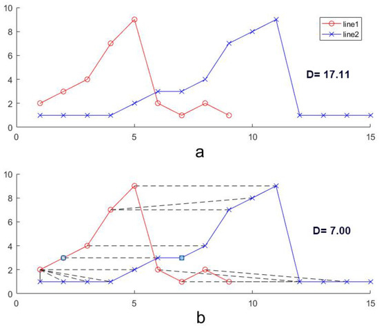
Figure 3.
Measuring curve similarity by the dynamic-time-warp method. (a) Traditional distance between classes (b) DTW distance between classes.
First, as the absolute value of the urban land area per capita among cities with differing sizes varies substantially, we normalized the urban land per capita (D’ in Equation (3)) for each city from 0 to 1 using its maximum and minimum values as follows:
where D is the original value of the urban land per capita at each buffer and and are the minimum value and maximum values of the urban land per capita of all the buffers in a city, respectively.
Next, the DTW distances were calculated for each city. The DTW was calculated by partially stretching or compressing the two time-series points to make them as similar as possible. After stretching or compression, the distance of each data point was calculated to obtain the similarity of the two time-series data [35]. Specifically, the DTW was used to find the optimally aligned bending path Φ for the two time-series data, X = (x1, x2,…, xn) and Y = (y,…, ym),. The bending curve could be described as:
where k = 1,…,T, Φx(k); Φy(k) ∈{1,…, t}, and the bending functions Φx(k) and Φy(k) map the time exponents of X and Y, respectively. For a given Φ, the average cumulative deformation of bending time series X and Y was calculated as:
where mΦ(k) is the weight coefficient, MΦ is the corresponding normalization constant, and Φx(k+1) ≥ Φx(k). By calculating the minimum value of the average cumulative deformation, the optimal bending path D(X, Y) is found, which is also the distance for the clustering.
Φ(k) = (Φx(k), Φy(k))
2.3.3. Analyzing Spatiotemporal Dynamics of Urban Land per Capita
We analyzed the features of the urban land per capita from 2000 to 2016. In terms of the features in 2016, we reported the mean values of China’s urban land per capita on multiple scales (among eight regions and three city sizes) and compared the urban–rural gradient characteristics of China’s urban land per capita among groups of cities. In terms of the temporal change, we reported the changes in the mean change in urban land per capita from 2000 to 2010 and from 2010 to 2016 and examined the shifts of cities between different urban–rural gradient groups.
3. Results
3.1. Characteristics of per Capita Urban Land in China in 2016
In 2016, the average per capita urban land in China was 118.9 m2/person. For regions, the average per capita urban land varied substantially (Figure 4). The averages in NEC and NWC were both higher than the national average and were 259.7 m2/person and 149.6 m2/person, respectively. The average value in NEC reached almost twice the nationwide average. The average values in ECC and ESC were nearly the same as the national averages, which were 113.0 m2/person and 113.8 m2/person, respectively. The average values in NCC, MRYLR, and MRYTR regions were smaller than the national values, i.e., 71.4 m2/person, 97.5 m2/person, 86.0 m2/person, and 89.1 m2/person, respectively.
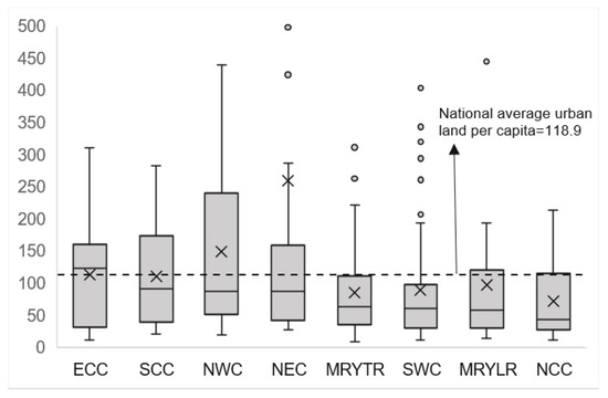
Figure 4.
Comparison of per capita urban land in different regions of China in 2016.
The per capita urban land among the three sizes of cities varied (Figure 5). In 2016, the average per capita urban land in the 113 large cities was 96.0 m2/person, which was approximately 23% lower than the nationwide average. Among these, the average per capita urban land in the large cities of ECC area was the largest, which was 138.2 m2/person. The average per capita urban land in the large cities of SWC was the smallest (58.4 m2/person). The average per capita urban land in the 115 medium-sized cities was 137.3 m2/person, which was approximately 13% greater than the nationwide average. The average per capita urban land was the largest in the medium-sized cities of NEC, i.e., 410.7 m2/person. In contrast, the average per capita urban land of medium-sized cities in ECC was the lowest at 56.3 m2/person. The average per capita urban land in the 75 small cities nationwide was 108.9 m2/person in 2016, which was 9% smaller than the nationwide average, for which the average per capita urban land was the largest in the small cities of MRYLR (183.4 m2/person) and smallest in the small cities of NCC (17.5 m2/person).
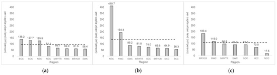
Figure 5.
The average per capita urban land among the three size groups of cities and regions: (a) large cities, (b) medium cities, and (c) small cities.
3.2. The Urban–Rural Gradient of per Capita Urban Land
Based on the clustering results (Figure 6), we can classify the urban–rural gradient of the per capita urban land into six types. The characteristics of the urban–rural gradient of the per capita urban land in large cities can be divided into two types, i.e., a mono-peak type and a fluctuating-increase type (Figure 7a,b). Among these, the major type was the mono-peak type, which included 90 cities in 2000, 104 cities in 2010, and 108 cities in 2016. Representative cities of this type included Beijing, Chengdu, and Wuhan. From the perspective of the urban–rural gradient, the per capita urban land curve in this type has one peak, after which the curve leveled off. The peak could be commonly found at a distance of 5 km from the urban center. After the 5 km peak, the value of the per capita urban land continued to decline and became steady until 20 km. The value of the per capita urban land at the urban periphery was proximately half of the peak value. The number of the fluctuating-increase cities was small, only amounting to 1 in 2000, 4 in 2010, and 4 cities in 2016. Representative cities included Shenzhen, Guangzhou, and Shanghai. From the perspective of the urban–rural gradient, there were several peaks of per capita urban land. The first peak occurred at a distance of15 km from the urban center, and the following peaks occurred at 20 km, 30 km, and 45 km.
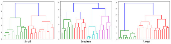
Figure 6.
The clusters of the urban–rural gradient of the per capita urban land among the three size groups of cities.
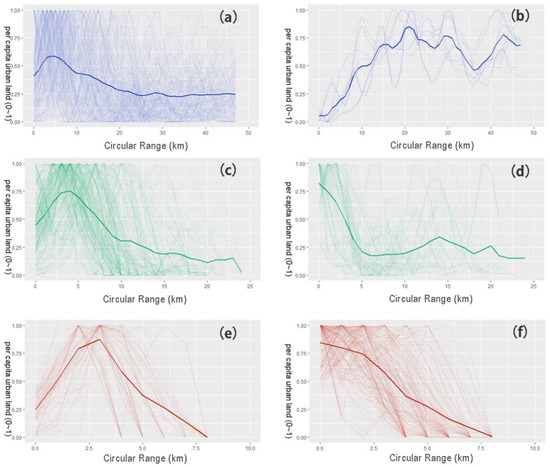
Figure 7.
Urban–rural gradient of per capita urban land among six types of cities: (a) large cities with a mono peak; (b) large cities with a fluctuating increase; (c) medium cities with a mono peak; (d) medium cities with a declining trend; (e) small cities with a mono peak; and (f) small cities with a decline trend. Note: the solid lines refer to the average value of each buffer.
The characteristics of the urban–rural gradient of per capita urban land in medium-sized cities can be divided into a mono-peak type and a declining type (Figure 7c,d). There were 34 mono-peak cities in 2000, 27 in 2010, and 20 in 2016. For instance, Jilin, Xichang, and Nanchong were classified into this category. From the perspective of the urban–rural gradient, there was likely to be a peak of per capita urban land at a distance of 4 km from the urban center, and then the value declined sharply until a 10 km distance from the urban center. There were 63 cities with a declining trend in 2000, 84 in 2010, and 95 in 2016. The representative cities were Sanya, Changchun, and Dali, which were mainly located in the central and western regions. From the perspective of the urban–rural gradient, there was a saddle area in its urban–rural gradient, which suggested that, after the bottom of the declining gradient, there existed a small increase and some small fluctuations thereafter. The declining-type cities reached the lowest value of per capita urban land at a distance of 5 km from the urban center, and the saddle reached its top at approximately 15 km.
The urban–rural gradient of the per capita urban land in small cities can be divided into a mono type and a declining type (Figure 7e,f). There were 19 small cities with a mono peak in 2000, 20 in 2010, and 23 in 2016; the representative cities included Lijiang and Ordos. Generally, the curve of per capita urban land had only one peak along the buffering rings and, after that peak, the value went down and declined until the urban periphery. The peak of per capita urban land for the mono-peak cities often occurred at a distance of 3 km from the urban center. There were 79 small cities with a declining trend in 2000, 62 in 2010, and 52 in 2016, for which Lianyungang and Ya’an were typical cities. This type was the major type of small cities. In general, the per capita of urban land for this type of city continued to decline until the edges of cities.
3.3. The Change in per Capita Urban Land in China from 2000 to 2016
At the national scale, the per capita urban land in China rose over time (Figure 8). The average per capita urban land nationwide was 110.2 m2/person in 2000, 112.6 m2/person in 2010, and 118.9 m2/person in 2016. The increase from 2010 to 2016 (5.7%) was greater than the increase from 2000 to 2010 (2.1%). In other words, the increase in per capita urban land has sped up in recent years.
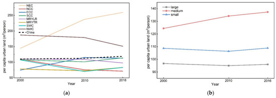
Figure 8.
The changes in per capita urban land among (a) regions and (b) cities of differing sizes.
At the regional scale, the per capita urban land in NEC increased steadily over time, rocketing from 144.7 m2/person in 2000 to 237.2 m2/person in 2010, an increase of 64%. The per capita urban land in the NCC, MRYLR, and NWC regions declined over time, among which the rate of decrease in NWC was the largest. The value of per capita urban land in NWC decreased from 187.1 m2/person in 2000 to 179.2 m2/person in 2010 (or decreased by 4.2%) and to 149.8 m2/person in 2016 (or decreased by 16.4%). In addition, the per capita urban land in the ECC, SCC, MRYTR and SWC regions fluctuated over time.
For cities of differing sizes, the per capita urban land of medium-sized cities showed a rising trend, whereas the per capita urban land in the other two types of cities was relatively stable. The value of per capita urban land in medium-sized cities increased from 124.4 m2/person in 2000 to 134.2 m2/person in 2010 and reached 137.3 m2/person in 2016. Correspondingly, the per capita urban land in large cities decreased from 96.7 m2/person in 2000 to 96.0 m2/person in 2016, declining by 0.7%, while the value of small cities increased from 109.7 m2/person in 2000 to 108.9 m2/person in 2016, rising by 0.02%.
3.4. The Change in the Urban–Rural Gradient of per Capita Urban Land in China from 2000 to 2016
From 2000 to 2010, 73 cities changed their types (Figure 9a1,a2; Table 1). Among these cities, 42 cities changed their sizes. Specifically, 13 medium-sized cities became large cities, 24 small cities changed to medium-sized cities, and 5 small cities switched to large cities.
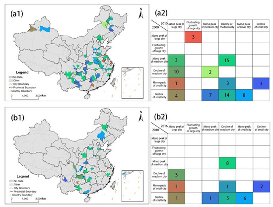
Figure 9.
The quantity and spatial distribution of type change from (a1,b1) 2000 to 2010 and from (a2,b2) 2010 to 2016. The colors in a2 and b2 were used for identifying corresponding cities in a1 and b1.

Table 1.
The change of city types from 2000 to 2016.
From the perspective of the urban–rural gradient, the major change was from a mono-peak medium-sized city to a declining-trend medium-sized city. Fifteen cities experienced such a change; representative cities included Hohhot and Lishui. In addition, 14 cities changed from declining-trend small cities to declining-trend medium-sized cities. In addition, the change from declining-trend medium-sized cities to a mono-peak large cities included 10 cities. Cities that experienced other types of changes ranged from 1 to 8.
From 2010 to 2016, 12 cities experienced size changes. For medium-sized cities, 3 cities became large cities. For small cities, 6 cities became medium-sized cities, and 2 cities became large cities. From the perspective of the urban–rural gradient, there were 28 cities that changed their types, which was fewer than the number of changed cities from 2000 to 2010 (Figure 9b1,b2; Table 1). Within a given size, the major change was from a mono-peak medium-sized city to a declining-trend medium-sized city (i.e., 8 cities). In addition, there were 2 cities that changed from a mono-peak small city to a declining-trend small city, and 6 cities showed the opposite.
4. Discussion
4.1. Characteristics of the Developed Method
The developed method has several merits. First, when compared with a traditional clustering analysis, the DTW-based clustering method can capture the urban–rural gradient of the per capita urban land. In analyzing the urban–rural gradients of the per capita urban land between cities, although the trends of the urban–rural gradients in different cities are similar, the locations of the peak value can be greatly different. If a traditional clustering method, such as K-means clustering, is used, it will calculate the distance between the absolute values of the urban land per capita in different circles and will not consider the similarity of curve trends. Here, DTW can cluster the urban–rural gradients of the per capita urban land with different ranges and with a similar trend. It works well for a nation-wide, per capita urban land dataset with a large variation in city sizes. Xuzhou, Qujing, Songyuan, and Chengde are classified as medium cities with a mono peak (Figure 10). Their per capita urban land data all show a trend of increasing first and declining thereafter, but their peak positions are different. The peak value of the per capita urban land is 4 km in Qujing city, 5 km for Songyuan City, 9 km for Xuzhou city, and 15–16 km for Chengde City, respectively. Through the DTW-based clustering method, these cities with a similar trend can be clustered into one type. However, if the K-means clustering method was used, they might not have belonged to the same type.
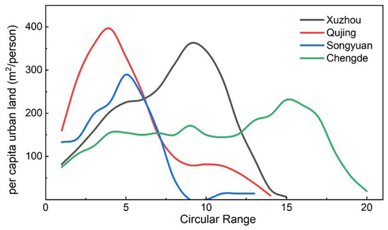
Figure 10.
The urban–rural gradients of per capita urban land in four mono peaks of medium cities.
Second, our method provides a richer type of rural–urban gradient and can be extended to study other indicators of the rural–urban gradient. Our study is based on clustering results and curve characteristics to derive curve types. When compared with previous studies on urban–rural gradients—in which the classification was usually based on established functions, such as the inverse S-shaped curve [26] and the Gaussian curve—this study performed the cluster classification of the urban–rural gradient curve of per capita urban land, which extended our understanding of the trend of human activities along urban–rural gradients.
4.2. Important Roles of Urban-Rural Gradient in per Capita Urban Land Use
Characterizing the urban–rural gradients of per capita urban land is of great significance to the understanding of urban sustainable development in theory and practice. First, this gradient reflects the intensity of human activity within a city. It can be used as an important input factor to analyze the impact of urban-land-use intensity on regional ecology and environment, such as the urban–rural gradient of an urban heat island [36], urban haze island [37], and urban acid island [38]. For example, along the urban–rural gradient, a heavy urban-heat-island effect and a large per capita urban land suggest dense buildings where green infrastructures should be improved.
Second, it can be used to identify polycentric cities. Among a number of cities such as Shanghai, Zhoushan, Shenzhen, and Guangzhou, the per capita urban land experiences multiple peaks from the urban center outward. These peaks are subcenters of these cities and can be readily identified by the urban–rural gradients of per capita urban land [39].
Third, the varying trends of the urban–rural gradient of the urban land per capita over time can be used as an important reference for urban planning. We analyzed a large number of cities of different sizes across the country and found some patterns of urban expansion in China, especially in the small- and medium-sized cities that are often overlooked. With the development of cities, we found that the urban–rural gradient of the per capita urban land in some Chinese cities changed, and most of the changes were from a mono-peak medium-size city to a declining-trend medium-size city, which suggested that the new growth of urban land was concentrated on the peri-urban areas in a low-density fashion. Most of the cities experiencing such changes were located in the central plain of China (MRYTR and MRYLR) and were driven by the rapid development of small- and medium-sized cities in central China in recent years [40]. For these low-density sprawling cities, policies should encourage the compact and vertical growth of urban land and prevent low-density development towards suburbs, which encroaches on natural habitats and affects regional ecosystem services [41].
Fourth, the urban–rural gradient of the urban land per capita can be further used to identify urban boundaries. For example, for a city with a mono peak, the density of urban land declines from the urban center to the urban periphery [26], which is consistent with the population density [42]. When the urban land per capita drops to a low value and maintains such a value for a relatively long distance, it suggests that we have reached an urban boundary. Previous researchers, such as Peng et al. [43] and Li et al. [19], used these distances to identify urban boundaries.
In addition, it is worth noting that the per capita urban land in China was lower than that of the world’s high-income countries/regions. According to the research of Tan et al. [4] in 2010, the average per capita urban land in large cities in high-income countries/regions, such as the United Kingdom and the United States, was more than 200 m2/person, while it was only 95 m2/person in China. Even in 2016, this value in China only increased to 96 m2/person. Such a gap means that, on one hand, the per capita urban land in Chinese cities may still have a large space for development [1] and, on the other hand, the intensive use of urban land in China is better than that in European and American countries. Moreover, the comparison of the per capita urban land among the three size groups of cities in China showed that medium-sized cities have the highest per capita urban land use. In other words, the sprawling urban expansion of medium scale deserves further attention [11].
4.3. Limitations and Future Perspective
This study proposes a clustering method based on the DTW to analyze the urban–rural gradient of the urban land per capita in Chinese cities. This method can be used to explore the trend of urban–rural gradients of the per capita urban land. The results can provide important scientific references for formulating urban-planning policies.
This study also has some limitations. First, the determination of an urban center is subjective. We chose the location of the municipal government as the city center, but some urban centers may not overlap with the location of their municipal government. It may lead to inaccurate estimation of the urban– rural curve. Second, the threshold value of the urban boundary was determined subjectively. Some small cities with a boundary smaller than 5 km were excluded in this study, which may lead to an overestimation of the boundaries of some large cities. In the future, the threshold value can be determined based on the urban-growth-boundary (UGB) method [44]. Finally, we did not quantitatively explore the shape of the rural–urban curve after clustering. In the future, we can quantitatively analyze the urban–rural gradient curve of the per capita urban land, and the per capita urban land form can be described by quantitative parameters.
5. Conclusions
To explore the patterns of the urban land per capita in different cities in China and its spatiotemporal changes over time, we developed a method to quantify and classify the urban–rural gradient of the per capita urban land and evaluated the changes of the urban per capita land in 2000, 2010, and 2016 among cities in China. First, we used the clustering method of DTW to explore the rural–urban gradient pattern of the urban land per capita in different cities in China. By focusing on the shape and trend of the data series rather than the absolute values, this method can more accurately capture urban–rural trends in urban land per capita than the traditional clustering method. Second, this method can be applied to other similar indicators along the urban–rural gradient.
The per capita urban land in China has increased over time. Its average value was 110.2 m2/person, 112.6 m2/person, and 118.9 m2/person in 2000, 2010, and 2016, respectively. The urban –rural gradient of the per capita urban land of 345 cities can be classified into six types. The major types were large cities with a mono peak, medium cities with a declining trend, and small cities with a declining trend, which accounted for 96.4%, 82.6%, and 69.3% of total large, medium, and small cities, respectively. For the northeastern and northwestern regions of China, their per capita urban land was relatively greater than that of the other regions. Therefore, the low-density sprawl of urban land in these regions should be strictly controlled, and the development of large cities should be encouraged from a single-center to a multi-center way.
Author Contributions
This research article has several authors; their individual contributions are specified below. Methodology, software, formal analysis, writing—original draft preparation, Y.L.; conceptualization, writing—original draft preparation, Q.H.; writing—review & editing, visualization, L.Z.; writing—review and editing, J.L., Y.S. and W.Z. All authors have read and agreed to the published version of the manuscript.
Funding
The research presented was supported by the National Natural Science Foundation of China (Grant Number 41971225), the Beijing Nova Program, and the Tang Zhongying Young Scholar Program (Qingxu Huang is a recipient of the program of Beijing Normal University).
Data Availability Statement
The data collected by the authors of this study are available on request from the corresponding author.
Acknowledgments
We express our gratitude to the anonymous reviewers and editors for their insightful and critical comments, which have improved the quality of the manuscript.
Conflicts of Interest
The authors declare no conflict of interest.
References
- Bakker, V.; Verburg, P.H.; van Vliet, J. Trade-offs between prosperity and urban land per capita in major world cities. Geogr. Sustain. 2021, 2, 134–138. [Google Scholar] [CrossRef]
- Camagni, R.; Gibelli, M.C.; Rigamonti, P. Urban mobility and urban form: The social and environmental costs of different patterns of urban expansion. Ecol. Econ. 2002, 40, 199–216. [Google Scholar] [CrossRef]
- Kasanko, M.; Barredo, J.I.; Lavalle, C.; McCormick, N.; Demicheli, L.; Sagris, V.; Brezger, A. Are European cities becoming dispersed?: A comparative analysis of 15 European urban areas. Landsc. Urban Plan. 2006, 77, 111–130. [Google Scholar] [CrossRef]
- Tan, M.; Li, X. Characteristics of Urban Land Per Capita of Major Countries in the World and Its Implications for China. J. Nat. Resour. 2010, 25, 1813–1822. [Google Scholar]
- Goldewijk, K.K.; Dekker, S.C.; van Zanden, J.L. Per-capita estimations of long-term historical land use and the consequences for global change research. J. Land Use Sci. 2017, 12, 313–337. [Google Scholar] [CrossRef]
- Wu, J.; Xiang, W.-N.; Zhao, J. Urban ecology in China: Historical developments and future directions. Landsc. Urban Plan. 2014, 125, 222–233. [Google Scholar] [CrossRef]
- Zhao, S.; Liu, S.; Xu, C.; Yuan, W.; Sun, Y.; Yan, W.; Zhao, M.; Henebry, G.M.; Fang, J. Contemporary evolution and scaling of 32 major cities in China. Ecol. Appl. 2018, 28, 1655–1668. [Google Scholar] [CrossRef]
- He, C.; Liu, Z.; Gou, S.; Zhang, Q.; Zhang, J.; Xu, L. Detecting global urban expansion over the last three decades using a fully convolutional network. Environ. Res. Lett. 2019, 14, 034008. [Google Scholar] [CrossRef]
- Kuang, W.; Du, G.; Lu, D.; Dou, Y.; Li, X.; Zhang, S.; Chi, W.; Dong, J.; Chen, G.; Yin, Z.; et al. Global observation of urban expansion and land-cover dynamics using satellite big-data. Sci. Bull. 2021, 66, 297–300. [Google Scholar] [CrossRef]
- Fan, P.; Yue, W.; Zhang, J.; Huang, H.; Messina, J.; Verburg, P.H.; Qi, J.; Moore, N.; Ge, J. The spatial restructuring and determinants of industrial landscape in a mega city under rapid urbanization. Habitat Int. 2020, 95, 102099. [Google Scholar] [CrossRef]
- Gao, B.; Huang, Q.; He, C.; Sun, Z.; Zhang, D. How does sprawl differ across cities in China? A multi-scale investigation using nighttime light and census data. Landsc. Urban Plan. 2016, 148, 89–98. [Google Scholar] [CrossRef]
- Jiang, H.; Sun, Z.; Guo, H.; Weng, Q.; Du, W.; Xing, Q.; Cai, G. An assessment of urbanization sustainability in China between 1990 and 2015 using land use efficiency indicators. Npj Urban Sustain. 2021, 1, 1–13. [Google Scholar] [CrossRef]
- Huang, Q.; Liu, Z.; He, C.; Gou, S.; Bai, Y.; Wang, Y.; Shen, M. The occupation of cropland by global urban expansion from 1992 to 2016 and its implications. Environ. Res. Lett. 2020, 15, 084037. [Google Scholar] [CrossRef]
- Fan, J.; Ren, Y. The Mechanism and Effect of Illegal Land Use on Sustainable and Intensive Land Use. China Land Sci. 2018, 32, 52–58. [Google Scholar]
- Grêt-Regamey, A.; Galleguillos-Torres, M.; Dissegna, A.M.; Weibel, B. How urban densification influences ecosystem services—A comparison between a temperate and a tropical city. Environ. Res. Lett. 2020, 15, 075001. [Google Scholar] [CrossRef]
- Ribeiro, H.V.; Rybski, D.; Kropp, J.P. Effects of changing population or density on urban carbon dioxide emissions. Nat. Commun. 2019, 10, 1–9. [Google Scholar] [CrossRef]
- Seto, K.C.; Christensen, P. Remote sensing science to inform urban climate change mitigation strategies. Urban Clim. 2013, 3, 1–6. [Google Scholar] [CrossRef]
- Kyttä, M.; Broberg, A.; Tzoulas, T.; Snabb, K. Towards contextually sensitive urban densification: Location-based softGIS knowledge revealing perceived residential environmental quality. Landsc. Urban Plan. 2013, 113, 30–46. [Google Scholar] [CrossRef]
- Li, M.; Verburg, P.H.; van Vliet, J. Global trends and local variations in land take per person. Landsc. Urban Plan. 2022, 218, 104308. [Google Scholar] [CrossRef]
- Fang, C.; Li, G.; Zhang, Q. The Variation Characteristics and Control Measures of the Urban Construction Land in China. J. Nat. Resour. 2017, 32, 363–376. [Google Scholar]
- Liu, J.Y.; Zhan, J.Y.; Deng, X.Z. Spatio-temporal patterns and driving forces of urban land expansion in china during the economic reform era. Ambio 2005, 34, 450–455. [Google Scholar] [CrossRef] [PubMed]
- Xu, X.; Zhang, Z.; Zhen, W.; Xu, S. Study on the index of urban per capita land use scale in China. China Soft Sci. 1999, 8, 3. [Google Scholar]
- Zhou, J. The causes and Countermeasures of low per capita urban construction land standard in China. China Anc. City 2019, 9, 9. [Google Scholar]
- Tan, M.; Li, X.; Xie, H.; Lu, C. Urban land expansion and arable land loss in China—A case study of Beijing–Tianjin–Hebei region. Land Use Policy 2005, 22, 187–196. [Google Scholar] [CrossRef]
- Zhou, K.; Tan, R.; Liu, Y.; Kong, X. Assessing of land-saving potential based on per capita construction land standards. Trans. Chin. Soc. Agric. Eng. 2012, 28, 222–231. [Google Scholar]
- Jiao, L. Urban land density function: A new method to characterize urban expansion. Landsc. Urban Plan. 2015, 139, 26–39. [Google Scholar] [CrossRef]
- Chen, Y. Derivation and generalization of Clark’s modelon urban population density using entropy—Maximising methods and fractal ideas. J. Cent. China Norm. Univ. (Nat. Sci.) 2000, 34, 489–492. [Google Scholar]
- Wang, Z.; Lu, C. Urban land expansion and its driving factors of mountain cities in China during 1990–2015. J. Geogr. Sci. 2018, 28, 1152–1166. [Google Scholar] [CrossRef]
- Ha, S.; Alimujiang, K. Analysis of the impact factors of urban heat island effect based on the intensive land use level. J. Glaciol. Geocryol. 2016, 38, 270–278. [Google Scholar]
- Yang, X.J. China’s Rapid Urbanization. Science 2013, 342, 310. [Google Scholar] [CrossRef]
- Liu, Z.; He, C.; Zhou, Y.; Wu, J. How much of the world’s land has been urbanized, really? A hierarchical framework for avoiding confusion. Landsc. Ecol. 2014, 29, 763–771. [Google Scholar] [CrossRef]
- Du, S.; He, C.; Huang, Q.; Shi, P. How did the urban land in floodplains distribute and expand in China from 1992–2015? Environ. Res. Lett. 2018, 13, 034018. [Google Scholar] [CrossRef]
- Seto, K.C.; Fragkias, M. Quantifying spatiotemporal patterns of urban land-use change in four cities of China with time series landscape metrics. Landsc. Ecol. 2005, 20, 871–888. [Google Scholar] [CrossRef]
- Liu, Y. Research and Application of Panel Data Clustering Method Based on Dynamic Time Warping. Stat. Res. 2016, 33, 93–101. [Google Scholar]
- Giorgino, T. Computing and Visualizing Dynamic Time Warping Alignments in R: The dtw Package. J. Stat. Softw. 2009, 31, 1–24. [Google Scholar] [CrossRef]
- Li, J.; Sun, R.; Liu, T.; Xie, W.; Chen, L. Prediction models of urban heat island based on landscape patterns and anthropogenic heat dynamics. Landsc. Ecol. 2021, 36, 1801–1815. [Google Scholar] [CrossRef]
- Zhu, L.; Huang, Q.; Ren, Q.; Yue, H.; Jiao, C.; He, C. Identifying urban haze islands and extracting their spatial features. Ecol. Indic. 2020, 115, 106385. [Google Scholar] [CrossRef]
- Du, E.; Xia, N.; Tang, Y.; Guo, Z.; Guo, Y.; Wang, Y.; de Vries, W. Anthropogenic and climatic shaping of soil nitrogen properties across urban-rural-natural forests in the Beijing metropolitan region. Geoderma 2022, 406, 115524. [Google Scholar] [CrossRef]
- Lv, Y.; Zhou, L.; Yao, G.; Zheng, X. Detecting the true urban polycentric pattern of Chinese cities in morphological dimensions: A multiscale analysis based on geospatial big data. Cities 2021, 116, 103298. [Google Scholar] [CrossRef]
- Wang, C.P.; Wang, H.W.; Li, C.M.; Dong, R.C. Analysis of the spatial expansion characteristics of major urban agglomerations in China using DMSP/OLS images. Acta Ecol. Sin. 2012, 1, 942–954. [Google Scholar] [CrossRef]
- Huang, Q.; Zhao, X.; He, C.; Yin, D.; Meng, S. Impacts of urban expansion on wetland ecosystem services in the context of hosting the Winter Olympics: A scenario simulation in the Guanting Reservoir Basin, China. Reg. Environ. Chang. 2019, 19, 2365–2379. [Google Scholar] [CrossRef]
- Clark, C. Urban Population Densities. J. R. Stat. Soc. Ser. A—Stat. Soc. 1951, 114, 490–496. [Google Scholar] [CrossRef]
- Peng, J.; Liu, Q.; Blaschke, T.; Zhang, Z.; Liu, Y.; Hu, Y.N.; Wang, M.; Xu, Z.; Wu, J. Integrating land development size, pattern, and density to identify urban–rural fringe in a metropolitan region. Landsc. Ecol. 2020, 35, 2045–2059. [Google Scholar] [CrossRef]
- Calthorpe, P.G.; Fulton, W.B. The Regional City: Planning for the End of Sprawl; Island Press: Washington, DC, USA, 2001; ISBN 1-59726-621-3. [Google Scholar]


Disclaimer/Publisher’s Note: The statements, opinions and data contained in all publications are solely those of the individual author(s) and contributor(s) and not of MDPI and/or the editor(s). MDPI and/or the editor(s) disclaim responsibility for any injury to people or property resulting from any ideas, methods, instructions or products referred to in the content. |
© 2022 by the authors. Licensee MDPI, Basel, Switzerland. This article is an open access article distributed under the terms and conditions of the Creative Commons Attribution (CC BY) license (https://creativecommons.org/licenses/by/4.0/).