Article

Mapping Urban Structure Types Based on Remote Sensing Data—A Universal and Adaptable Framework for Spatial Analyses of Cities

1
Department of Geosciences, Institute of Geography, University of Tübingen, 72070 Tübingen, Germany
2
Remote Sensing Data Center (DFD), German Aerospace Center (DLR), 82234 Weßling, Germany
*
Author to whom correspondence should be addressed.
Land 2023, 12(10), 1885; https://doi.org/10.3390/land12101885
Submission received: 6 September 2023 / Revised: 3 October 2023 / Accepted: 5 October 2023 / Published: 7 October 2023
(This article belongs to the Special Issue Urban Morphology: A Perspective from Space)

Abstract

:
In the face of growing 21st-century urban challenges, this study emphasizes the role of remote sensing data in objectively defining urban structure types (USTs) based on morphology. While numerous UST delineation approaches exist, few are universally applicable due to data constraints or impractical class schemes. This article attempts to tackle this challenge by summarizing important approaches dealing with the computation of USTs and to condense their contributions to the field of research within a single comprehensive framework. Hereby, this framework not only serves as a conjunctive reference for currently existing implementations, but is also independent regarding the input data, spatial scale, or targeted purpose of the mapping. It consists of four major steps: (1) the collection of suitable data sources to describe the building morphology as a key input, (2) the definition of a spatial mapping unit, (3) the parameterization of the mapping units, and (4) the final classification of the mapping units into urban structure types. We outline how these tasks can lead to a UST classification which fits the users’ needs based on their available input data. At the same time, the framework can serve as a protocol for future studies where USTs are mapped, or new approaches are presented. This article closes with an application example for three different cities to underline the flexibility and applicability of the proposed framework while maintaining maximized objectivity and comparability. We recommend this framework as a guideline for the use-specific mapping of USTs and hope to contribute to past and future research on this topic by fostering the implementation of this concept for the spatial analysis and a better understanding of complex urban environments.

1. Introduction

Undoubtedly, urbanization is among the largest challenges of the 21st century. According to latest estimates of the United Nations, over two-thirds of the global population will live within cities by the year 2050 [1]. This will put additional pressure on the process of urban planning to continually provide sustainable and healthy living conditions, public services, and an effective use of resources [2,3]. The most urgent fields of action involve the increasing population, regarding both number and density, the accessibility of public services and healthcare, and environmental quality, which all emerge at different demographic, temporal, and spatial scales. In addition, the latest studies underline that new problems will emerge at different social, spatial and temporal scales within the context of global warming, especially in urban areas, which at the same time are one of the biggest sources for environmental pollution [4,5,6,7].
Concepts such as information-based or data-driven planning have emerged to support decision-making and governance based on empirical evidence [8,9,10]. However, data availability is strongly dependent on the sector: while data on traffic, transportation or mobility can easily be collected from mobile phones or smart sensor networks in real-time [11], other topics that are closely related to sustainable development, such as environmental degradation, socio-economic inequality or vulnerability to natural hazards, are more complicated to monitor and require different forms of assessment [12,13]. Among others, methods of Earth observation and geospatial analysis have proven to be a cost-effective alternative to in situ data collection which allow to researchers to obtain reliable, accurate and objective information on urban areas within both scientific and applied frameworks [14,15,16,17,18]. Their contribution to a broad variety of applications has been demonstrated in numerous studies, for instance, in the monitoring of urban changes [19], population densities [20], green spaces [21], water resources [22], impervious surfaces [23], taxation [24], urban heat [25], or informal settlements [26].
However, all of these studies identified cities as complex spaces with an interior differentiation that must be considered. As highlighted by Reba and Seto (2020), who undertook an extensive review of studies on urban land monitoring, only 13% of their investigated studies distinguished between multiple intra-urban classes [19]. Also, Zhu et al. (2019) named urban heterogeneity as one of four strategic future directions for urban remote sensing research [18]. However, most observed phenomena inside cities are spatially continuous and therefore challenging to capture and store from a data perspective [27,28,29]. At the same time, many of the reported problems are observed to equally affect municipalities across the entire globe, thus demanding a systematic and scalable approach, which not only allows findings (e.g., on changes related to climate) to be more comparable between cities of different regions or even states, but in an ideal case, also transferable [30].
To cope with these challenges, different approaches have been proposed to define aggregated spatial units that are homogenous concerning the information of interest. Within this field, the concept of urban structure types (USTs) was introduced in different forms. An early definition was provided by Wickop et al. (1998) which viewed urban structure types as an intermediate element between the scale of a single building and the more generalized classification of urban land use or land cover [31]. As one of the earliest authors on this topic, Taubenböck et al. (2009) delivered evidence on the correlation between the physical structural units of a city and socio-economic parameters collected in the field—in their case, monthly income and property prices [32]—to conclude that regional planning or risk and vulnerability assessments can be assisted by a systematic view at a city as provided by satellite imagery. For instance, Patino et al. (2014) were able to correlate urban layout and land cover composition with crime rates in Medellin, Colombia [33], and Dang et al. (2018) highlighted a negative linear relationship between the number of green spaces and deaths attributed to urban heat within Ho Chi Minh City [34]. Similarly, Jiang et al. (2021) found that several indicators of built-up structure were significantly associated with suicide rates within Hong Kong, more precisely the distance to the nearest urban center, the distance to the nearest railway station, and the average housing area per person [35]. Urban structures not only correlate with human health, but also with information associated with sustainable urban planning, as demonstrated by Downes (2022), who showed how mapping these urban structures can help to identify the current status and future needs for environmental infrastructure provision in different parts of Da Nang [36].
As shown by the examples given above, there is a wide field of different approaches and scientific targets related to the description and delineation of urban morphology. To summarize these, Blum and Gruhler (2011) claimed that mapping urban structures can serve three different purposes [37]:
(a) Link: Urban structures can be defined to directly relate the morphology of a defined spatial unit of analysis and its physical characteristics (land use, albedo, energetic properties), such as the concept of Local Climate Zones (LCZ) proposed by Stewart and Oke (2012, see Section 2.3) [38,39].
(b) Vehicle: Observing gradual or classified changes in the urban structure as a proxy for the variations in socio-economic conditions within a city. This idea was supported by Banzhaf and Hofer (2008), who viewed urban structures as a spatial unit to analyze economic, ecologic and social phenomena to support the development of sustainable adaptation strategies [40].
(c) Interface: Using morphologically defined areas as a “boundary object” [41] fostering communication and transferability between different research disciplines or medium for stratified sampling of field observations to equally represent all types of structural elements, or populations within a city [42].
Accordingly, there is no universal scheme of urban structure types because they differ with respect to the field of research, their computational derivation and their semantic definition. However, their contribution to the reduction in complexity, the support of decision making and the development of interdisciplinary research is widely acknowledged [43,44,45]. However, while most of the developed nations have national programs for the development of geospatial data infrastructures, many rapidly developing cities in countries in the Global South have the highest need for data and information which can feed into decision making and urban planning and foster transitions towards the achievement of the Sustainable Development Goals [46,47,48,49]. At the global level, this demand for data is increasingly tackled by openly available datasets, such as the Global Human Settlement Layer [50], the World Settlement Footprint [51], or WorldPop [52]. Their most striking benefit for both scientific and applied applications is their consistency concerning data sources and methods, which makes them an invaluable input for comparative studies at the national, continental and global scale [53]. However, these are not applicable for the characterization of patterns and processes of individual cities, especially at their transition into peripherical and rural parts [54,55,56], which are the most dynamic and relevant with respect to sustainable urban development in cities of the Global South [57].
Studies of several disciplines have therefore underlined the need for transferable approaches to accurately characterize inner-urban morphologies at an abstracted and comparable, but still local, level, at best at the building or neighborhood scale, to support decision making related to urban development, including transit-oriented development facilitating sustainability transitions on urban and regional levels [58], urban climate risk assessment [59], urban sprawl and strategies for green urban growth [60], urban architecture and design [61], mobility and transportation [62], or age-responsive planning [63]. Understandably, global datasets do not meet the demands of such specialized applications. Additionally, cities with different morphogenetic and cultural characteristics may not always fit into global classification schemes and might require adaptions with respect to cultural specifications [64,65], the desired spatial scale [66], and a targeted spatial unit of analysis or reporting [67,68].
The aim of this article is to respond to the call for a more generalized framework to map USTs raised by Wang (2022) [56], which is universally applicable and consolidates important studies, thereby condensing their contributions to the field of research. This framework is independent of input data, spatial scale, or the targeted purpose of mapping, making it a versatile reference protocol for future studies. It especially addresses the situation of data-scarce environments by highlighting how satellite imagery and geospatial information can feed into such concepts, thus empowering researchers and planners in cities of the Global South to perform data-driven information generation and decision making.
In Section 2, a literature review outlines past UST mapping efforts and their scientific contributions, which are then summarized in the proposed framework in Section 3 depending on different strategies as observed in other studies and based on the user’s capabilities and needs. Section 4 demonstrates its applicability for the comparison of three selected cities before a summary is drawn in the last part to address the lessons learnt and define future research needs.

2. Review of Existing Frameworks

To build upon the valuable ideas and findings of preliminary studies, this chapter will briefly summarize relevant concepts which have already been proposed, introduce their advantages and shortcomings, and compare them with respect to the following indicators, which refer to input data, the conceptual implementation, and the class scheme:
Input data
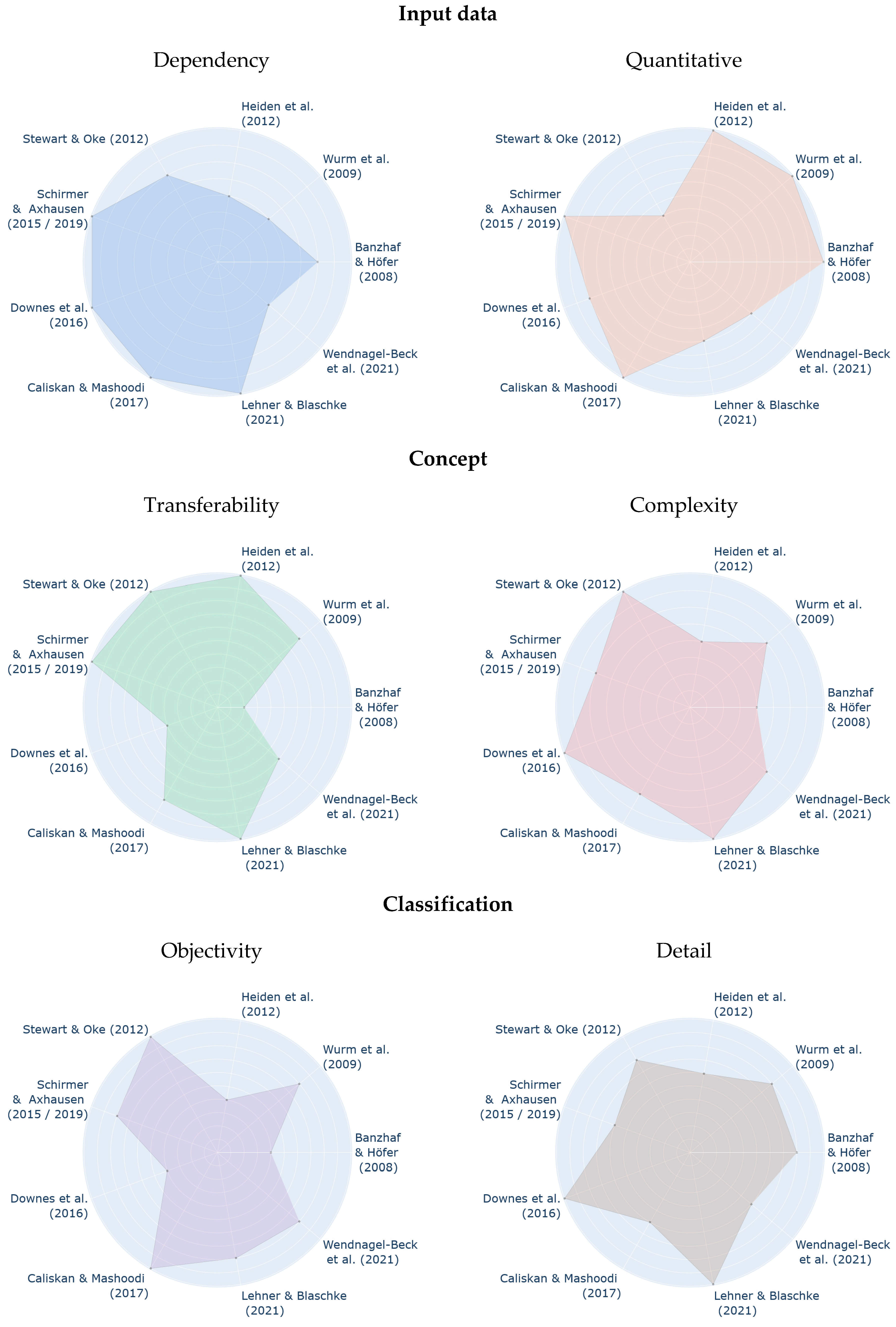
  • Dependency: Is the concept dependent on a certain type of input data (1: specific data required) or is it universally applicable (5: any data)?
  • Quantitative: Is the concept purely theoretical (1: concept only) or data-driven (5: fully quantitative)
Conceptual implementation
  • Transferability: Are the USTs linked to a certain city or region (1: locally valid) or is the concept transferable to any study area (5: fully transferable)
  • Complexity: Is the delineation of USTs computationally complex (1: experts only) or can it be achieved by anyone (5: easy or adjustable implementation)
Classification
  • Objectivity: Is the assignment of classes subject to interpretation (1: fully subjective) or is it defined objectively (5: automated or value-based assignment)?
  • Level of detail: Is the inner-urban differentiation coarse (1: few classes) or detailed (5: many classes)?

2.1. Early Concepts and Spatial Theories on Morphology

The idea of a consistent and hierarchical classification of land use and land cover based on satellite imagery is not new and was, among others, initially proposed by the US Geological Survey in 1976, who defined nine main classes (Level 1), of which the first was “Urban or built-up land”, containing seven sub-classes (Level 2) [69]. However, these were mostly linked to the actual uses (e.g., residential, industrial, commercial), which are not always linked to distinct spectral characteristics and therefore are only detectable via the visual interpretation of VHR imagery. Also, addressing the need for a comparable measure of urban space UN Habitat provided a globally applicable definition of a city and its morphology [70] solely based on the density of built-up areas, distinguishing between urban built-up areas (>50%), suburban built-up areas (25–50%) and rural built-up areas (<25%), with further distinction from fringe open space, captured urban space, and rural open space, which are defined by means of the metric distance or neighborhood measures. The latest approach of this type is the EAGLE concept, which hierarchically combines elements of land cover and land use with a more flexible description of land characteristics, such as management type, spatial patterns, ecosystem types or legal status, but again, with little focus on urban environments [71].
Caliskan and Mashoodi (2017) bridged the theoretical concept of urban coherence with the definition of specific spatial attributes to allow its data-driven derivation [72]. They focused on spatial proximity and consistency, utilizing the Gini Simpson index for comparative analysis across urban settings. Using data on buildings, street-blocks, streets, pedestrians, and green areas, they quantified coherence in three Rotterdam neighborhoods. Their concept offers mathematical reproducibility and aids in understanding functional efficiency and vitality in urban environments, adding value to socio-scientific analyses.
Similarly, Schirmer and Axhausen (2015) recognized the contribution of geospatial data for the characterization of urban morphology as an input for studies dealing with human behavior, land prices, or simply urban planning [73]. They understand cities as compositions of blocks, buildings and streets and conceptualize how they can be modeled by spatial data to hierarchically derive second-order measures, such as density, homogeneity, centrality, or accessibility, at the neighborhood or municipal level. They later extended this concept with a more comprehensive data model and suggestions on how to cluster the quantitative attributes into spatially homogeneous urban morphologic zones as inputs for modeling studies [74].

2.2. Fundamental Remote Sensing-Based Studies

Banzhaf and Höfer (2008) introduced an early scheme using aerial imagery to derive urban structure types [40]. This approach delineated buildings from the imagery and aggregated them at the neighborhood level based on road network information, resulting in fifteen classes encompassing architectural, morphogenetic, and land use characteristics (e.g., Wilhelminian style or shopping centers). While this method proved time- and cost-effective, its transferability was limited due to its city-specific nature and manual refinement in Leipzig.
Wurm et al. (2009) proposed a modular approach primarily utilizing very-high-resolution (VHR) satellite imagery alongside digital surface models (DSM) for Cologne and Dresden. They derived built-up areas, which were subsequently divided into two levels of higher detail, resulting in nineteen urban structure types. These types encompass both objective descriptions (e.g., small multi-story buildings) and subjective classes (e.g., “old towns” or “mixed-use areas”), which were refined in subsequent studies [75]. This hierarchical structure allows users to tailor the level of detail, enhancing adaptability and transferability. Additionally, the object-oriented analysis accommodates relationships with superior or neighboring objects, incorporating a crucial aspect of morphological analysis [76].
To increase the information content of image data, Heiden et al. (2012) used hyperspectral imagery in combination with DSMs which allowed them to identify roof and pavement materials as well as vegetation in the city of Munich [77]. These served as inputs for detailed morphological features of building blocks, including the degree of imperviousness, the percentage of non-built-up, fully impervious surfaces, the percentage of partially impervious surfaces, building density, vegetation density, building volume, and vegetation volume. Based on these features, six urban structure types were classified. As both the derivation of features and the naming of the final classes were highly objective and city-independent, this work can be considered the first fully transferable approach for UST mapping.
The currently most detailed and thorough concept was presented by Lehner and Blaschke (2019), who first reviewed numerous studies on UST mapping and acknowledged the challenge of deciding between a concept which ideally describes a specific city or a universally applicable concept [44]. They concluded that a generic scheme should be applicable to any city worldwide, should not rely on specific input data and should not refer to land use in any way. Their scheme is highly hierarchical and consists of six levels of detail with nineteen classes in the most detailed level. They additionally suggested input data for each of these six levels which fit the desired spatial scale and whether height information is required or not. Although it does not come with a distinct case study, its relevance for urban planning was reported to be high based on expert interviews.

2.3. Concepts for Specific Purposes

This section briefly lists central works within the context of UST mapping which were selected because of their scientific impact, unique ideas, or integrated approach with no claim to be exhaustive. It closes with a comparative table of all concepts introduced in Section 2.
The currently most prominent and highest adapted is the concept of Local Climate Zones (LCZ) by Stewart and Oke (2012) [38]. This concept consists of ten main morphologic built types which are defined by the density of buildings and their average height. These are complemented by another seven classes related to land cover (vegetation, soil, water), so that these can be linked to specific surface energy and radiation balance characteristics to reduce the complexity of urban climate studies. Despite its narrow thematic focus, this concept was quickly adopted by studies outside the urban climate domain: Zhu et al. (2022) used the LCZ scheme in combination with the World Settlement Footprint (WSF) to analyze urban morphologies at the global scale [78]. They concluded that there are seven morphological city patterns: European cities, cities of the Islamic world, predominantly Chinese cities, predominantly African cities, predominantly American-African cities, European-African-Asian cities, and very large cities. Sapena et al. (2021) applied the LCZ concept to 31 German cities to compare their morphologic composition to socio-economic variables related to education, health, living conditions, labor, and transport to assess the predictive contribution of urban structures for quality of life indicators [79]. As the concept gained immense attention, derivates and advancements emerged, such as its implementation within the World Urban Database and Access Portal Tools (WUDAPT) [80] or automated derivations based on convolution neural networks (CNNs) and openly available Sentinel-2 data [81].
As an alternative to automated and fully generic approaches, Downes et al. (2016) suggested a way to embed USTs into risk adaptation and planning in Ho Chi Minh City based on twelve Vietnamese building archetypes [82]. These were used as base information together with several spatial indicators (e.g., building density, height, or degree of imperviousness) for a fully visual interpretation of VHR satellite imagery resulting in a total of 82 different urban structure types within the city with a strong focus on land use. The authors argue that while this approach is less transferable and strongly dependent on the experts’ interpretation, it provides higher value for spatial planning, decision making and the evaluation of disaster risk and resilience.
Considering all previous aspects, Wendnagel-Beck et al. (2021) [83] combined spatial information, legal frameworks and statistical data to examine how climate adaptation plans in Karlsruhe and Berlin consider physical information on urban structures, but also social structures related to human vulnerability to assess climate risks and to identify adaptation needs and actions. For this, they not only classified the cities into twelve predefined urban structure types, but also categorized them regarding their potential for climatic stress and exposure to heat. Using USTs as a medium for the projection of vulnerabilities in the year 2050, they were able to identify needs for action and to develop sustainable adaptation pathways.
Figure 1 visualizes the reviewed concepts with respect to the six criteria. As displayed in the spider plots, all approaches have strengths and downsides, and most of them are strongly capable of being primarily fed by geospatial data, which makes them largely scale-independent and spatially transferable. However, they strongly vary regarding the complexity of their computation and the flexibility of the class scheme, for example when it comes to the definition of locally adjusted classes. As no concept can fulfill all aspects equally, we introduce a framework in the next chapter which incorporates a wide range of requirements, starting from easy and locally precise to fully automatable and globally valid. Through this, we seek to summarize the benefits of all presented aspects under a joint umbrella based on a clear structure to empower scientists, planners, and users of all domains to implement an urban structure type classification which ideally fits their capabilities and needs.

3. Proposed Framework

This chapter summarizes approaches to UST mapping within a systematic framework which is adaptable and based on quantitative processing and analysis. It is understood as a bottom-up approach starting at the building level as a basic spatial unit of urban morphology but will outline different procedures to achieve a final assignment of USTs.
Figure 2 shows the general structure of our proposed framework, which also defines the subsequent sections. It starts with a description of the built-up environment (Section 3.1) and the definition of a mapping unit (Section 3.2). The most important aspect is the subsequent enrichment of these mapping units with attributes, which allow us to distinguish between the different units based on defined characteristics (Section 3.3). Based on these features, a final assignment of classes can be conducted, again in numerous ways (Section 3.4). As recommended, but not ultimately required, steps, validation and cartographic presentation (Section 3.5) follow this.

3.1. Building Morphology

As a main finding of the literature review of the previous chapter, we see morphologic aspects as the most important information for the mapping of urban structures. Although there are studies which argue that not all aspects which might be relevant for the spatial analysis of cities might be attributable to the built-up structure, they are still the most objective and consistent measure and, compared to socio-economic information (e.g., number of residents, demography, employment), are comparably easy to retrieve with methods of spatial data processing. Moreover, as also presented in the introduction, their correlation with socio-economic parameters can be surprisingly high. As our aim is to use USTs as inputs or proxies for subsequent information, we suggest buildings as the main mapping unit for a bottom-up approach. Ideally, they are represented as polygons (vector format), which delineate the footprint of each individual building. As an alternative, especially in data-scarce environments and large cities, the general outline of all (single and adjacent) build-up structures could be used to describe changes in the structural morphology, either as a polygon or as a raster model. If no two-dimensional information is available at all, buildings could also be represented by single points to deliver information on their density (see Section 3.3.2). An example of different data types on buildings which could be used within this framework is given in Figure 3. As the presented approach is designed to be as transferable as possible, no attribute information (e.g., heights) is expected to be within these building data.

3.1.1. Official Building Data

In an ideal case, data on building footprints are provided by the municipality. However, as highlighted by Biljecki et al. (2021), there are barely any governmental data sources on cities in countries of the Global South [84], while these would benefit the most from a solid spatial data infrastructure. This was confirmed by Zhou et al. (2022), who reported strong inequalities between cities of the Global North and the Global South when it comes to the height attributes of buildings [85].
As another relevant aspect, local datasets might provide the highest geometric accuracy for buildings but cannot be used in studies where urban structures of different cities are compared. For instance, Taubenböck et al. (2017) underlined the necessity for a harmonized data source for their comparison of urban polycentricity of different German cities [86]. Accordingly, urban structure types can only be used for the transfer of the characterization of different cities if they were derived from homogenous base data. Therefore, it depends on the study design if official building data are to be preferred over alternative sources (next subsections) of potentially lower data quality.
Efforts to harmonize building data at the administrative level exist, for example within the INSPIRE directive which standardizes geospatial data infrastructures between all member states of the European Union, where building footprints are explicitly mentioned in guideline D2.8.III.2 [87]. It contains a detailed description of how buildings are to be mapped, stored and attributed (building characteristics and metadata), but the status of implementation and the public access to such data still strongly vary between the member states [88].

3.1.2. Openly Available Building Footprints

If no official data on building outlines are available, secondary sources can be utilized. Table 1 gives a summary of the most important secondary data sources for different regions. However, as with administrative data, regional differences regarding accuracy and completeness exist, so users are required to check technical descriptions and scientific publications for exact information on data quality. The most popular is the OpenStreetMap (OSM) project, which globally collects spatial data on roads and infrastructures, fully collected by volunteers [89]. All data are publicly available, GIS-ready and based on a simple but consistent scheme for metadata. Its greatest advantage is that all buildings are manually digitized, and each database upload is documented by metadata, and is therefore reviewable. On the downside, studies show that the distribution of OSM data is strongly uneven at a global level and that the data for many regions are still incomplete or of poor quality, especially with respect to building footprints [90,91]. Efforts have been undertaken to close gaps with respect to a more extensive attribution based on mobile apps, such as StreetComplete [92] or MapSwipe [93], the systematic data contribution for under-represented regions within mapping events (‘mapathons’), especially in the humanitarian domain [94,95], or general data ingestion based on new methods of artificial intelligence and machine learning [96,97]. Due to its extensive metadata system, all changes are tracked, providing insights into data quality and up-to-dateness [98].
To strategically address data scarcity in developing countries, Google released a building dataset in 2021 [99] containing 1.8 billion building footprints retrieved from satellite imagery within Africa, South Asia, South-East Asia, Latin America and the Caribbean. Each building comes with a confidence estimate to communicate the expected data quality to potential users. A detailed quality report is available to inform about regional differences in availability, completeness, and systematic errors.
Various initiatives exist which try to maximize data harmonization at the continental scale based on combinations of data from OpenStreetMap and governmental datasets. As one popular example, EUBUCCO is an open collection of building footprints for all European cities, containing over 202 million buildings [100]. Additionally, three attributes are potentially stored, but not equally among all buildings: height (73% complete), year of construction (24% complete), and building type (46% complete). All data are well documented and available for download in the open geopackage format. A similar attempt is undertaken within the Digital Building Stock Model (DBSM [101]), which aims at the development of a seamless pan-European map of building footprints in vector format, primarily to address questions revolving around energy provision, transition and performance of single buildings. As a project directly funded by the European Commission, it will benefit from the provision of authoritative data by Member States and is expected to achieve the highest quality in terms of actuality and harmonization. An example of a similar procedure is the Multi-Temporal Building Footprint Dataset (MBTF-33) published by Uhl et al. (2022), which collected building data from administrative, county- or state-level institutions for 33 counties in the United States and released them, enriched by the year of construction, to allow detailed analyses of temporal changes in the building morphology of US cities [102].
Opposing the efforts to collect and standardize administrative data, Microsoft started to extract building footprints based on VHR satellite images within Bing Maps using artificial intelligence and high performance computing [103]. Large extents of the US and many other countries have been made available since then via GitHub in GeoJSON format, accompanied by an extensive quality assessment. A different approach was followed by Feng et al. (2023), who used Sentinel-2 imagery and spatial upsampling techniques to derive 86.3 million individual buildings at a spatial resolution of 2.5 m for large parts of China [104]. Many more datasets are available for other regions or distinct applications, but due to the pace of new developments, the aforementioned shall serve as representative examples. It is advisable to test and compare in case more sources are available for the desired region. Figure 4 shows how quality and the degree of generalization can vary among different datasets using the example of the central business district of Kigali in Rwanda. It demonstrates how OSM is partly incomplete and coarse, especially in the transition into residential areas.

3.1.3. Generation of Building Footprints

Especially in countries of the Global South, data on buildings might not be collected and publicly shared by administrations or covered by comprehensive datasets as presented in the previous subsection, and the available data may not meet the quality requirements for the desired study. This is often the case in rapidly developing cities where building stocks change at a high pace. In such cases, one option remaining is to create a new dataset of building footprints. The easiest way to achieve this is through manual digitization based on satellite imagery, which is labor-intensive and time-consuming, but might result in the most precise results [105]. As another advantage, there is no need for complex data processing techniques and high-performance computers, because digitization can be performed in any desktop mapping software, and local knowledge can be integrated into the interpretation process so that the digitized buildings ideally meet the study’s needs and can be enriched with attribute data (e.g., building type) during the mapping process. Concludingly, manual digitization can be a viable option if the size of the city is small to medium or if many persons are available for the digitizing tasks. However, especially when many contributors are involved, guidelines are required to grant for data consistency, for example in the form of interpretation keys and digitization protocols [106].
Methods for the automated or semi-automated extraction of building footprints from raster data are manifold and address diverse kinds of input data. Approaches based on VHR optical data as the most common input were recently summarized by Li et al. (2022), who reviewed 417 articles for their techniques, desired outcomes, and applications [107]. Besides multispectral data, height information retrieved by means of airborne laser scanning, unmanned aerial vehicles (UAVs) or stereo-photogrammetric methods are often used in the form of digital surface models (DSMs) to delineate built-up objects in urban areas [108,109,110,111,112,113], but also less conventional approaches exist, for example using synthetic aperture radar (SAR) imagery [114] or extracting building stock from topographic maps [115]. Regarding the methodology, a paradigm shift can currently be observed: while object-based image analysis (OBIA [116]) has been the most effective and frequently used method for the last two decades, new techniques based on artificial intelligence have emerged which no longer treat image data as spatial concepts, but rather exploit the massive potential of deep learning (DL), which allow us to detect patterns in data more effectively [117]. However, as stated by Lang et al. (2018), OBIA and DL are not mutually exclusive concepts, but rather grow together and will continue to benefit from each other [118].
One of the largest challenges for the automated extraction of building footprints arises in densely built-up environments where buildings are not isolated or detached but tangential to each other. In such cases, segmentation-based approaches often fall short of delineating the single buildings because of missing visible boundaries. If this is not sufficient for the intended analysis, buildings have to be separated manually, or with the help of tiling algorithms, such as Thiessen polygons around centroids [119], or in an ideal case, based on cadastral borders which are assumed to coincide with building boundaries (Figure 5).
As a last step, post-processing could be required, because building outlines retrieved from satellite imagery with OBIA are mostly irregular without straight edges. To achieve more rectangular building shapes, generalization tools can be applied which reduce geometric artefacts based on shape indices or iterative smoothing [120]. An extensive review of the quality and uncertainties of urban elements mapped from satellite imagery was provided by Wang et al. (2022) [121].

3.1.4. Proxy Datasets

If no information on buildings can be retrieved or generated because of a lack of data or capacities, or if simply time is short, proxy information can be utilized to describe urban morphology. Depending on the spatial scale and design of the targeted subsequent analysis, different data sources can be exploited. For the description of built-up areas at the local and regional scale, substantial groundwork has been laid by datasets of the Global Human Settlement Layer (GHSL [122,123]), the Global Urban Footprint (GUF [124]), or the World Settlement Footprint (WSF [51]). All of them provide global coverage, allowing for their usage within comparative studies on different cities’ morphology. They exist at different levels of detail, and present various types of information, starting with the pure extent of built-up areas (including open areas within cities), ranging over heights and volumes, to entire secondary or modeled information layers, such as population density or classified urban space. Examples are given in Figure 6. Besides these datasets published by public institutions, there are many more containing data with global or regional coverage for distinct urban morphology analysis, for example provided by Li et al. (2021), who modelled the global three-dimensional building structure (building footprint, height and volume) at a spatial resolution of 1 km with high accuracy (R2 of 0.89, 0.73, and 0.84, respectively). Furthermore, many initiatives seek to provide consistent data at the continental level. An example for national datasets was presented by Frantz et al. (2021) who published a raster containing built-up heights with a spatial resolution of 10 m for the entirety of Germany retrieved by openly available Copernicus data with an estimated mean height error of around 3.6 m [125].
Table 2 gives a brief overview of currently available datasets which can be used within this framework as a substitute for detailed vector building footprints. As stated before, the aim (single city vs. many cities) and spatial scale (local, regional, continental or global) of the study strongly define whether such data of coarse detail are sufficient or not and whether their completeness and consistency are of value.
To conclude with options regarding building morphology, Table 3 comparatively lists the different options including their advantages and challenges.

3.2. Definition of a Mapping Unit (Block)

The second step after the collection of building data is the definition of a spatial unit which can be used to discretize the continuous nature of the city [121]. This is necessary because analyses based on the level of individual buildings alone do not allow for a characterization of blocks, neighborhoods or otherwise defined parts of a city, and the concept of urban structure types per se involves the step of spatial aggregation [40,44]. Different approaches exist, but again, how this is achieved is dependent on both data availability and the respective aim of the study. Within this framework, we use the term “block” as a representation for any kind of spatial zoning, as described in the following.

3.2.1. Administrative Boundaries

The most straightforward division of cities is following administrative boundaries which are provided by city administrations, and therefore this comes closest to applications of urban planning. Accordingly, findings based on mapped USTs at the level of official districts have a higher potential to be considered when it comes to planning recommendations and their implementation [136]. Similarly, land-use plans can be used as a spatial division of a city [59]. If the city of interest does not provide official boundaries, the open GADM database is a suitable alternative which hosts administrative divisions of nearly all countries at various levels up to the neighborhood scale of cities, stored as harmonized ESRI shapefiles or in the open GeoPackage format [137]. A major downside of using administrative boundaries is that there can be substantial differences in their size, not only between cities of different countries, but also within cities, which can cause incomparable statistics in the later parametrization of the units (as demonstrated in Section 4.1). This is strongly linked to the modifiable areal unit problem (MAUP), which states that changes in the mapping unit unpredictably change the statistics of underlying data [138]. Therefore, it must be carefully checked if the administrative divisions are a spatially and statistically robust representation of the city’s morphology, and more importantly, comparable between cities of different countries. The impact of the MAUP with respect to quantitative descriptions of urban morphology is discussed in detail by Zhang and Kukadia (2005) [139]. Parcels represent the most detailed form of administrative boundaries which are precise because of their legal character, but they are rarely shared publicly and probably too detailed for the distinction at the neighborhood scale (Figure 7B). Yet, they can be viewed as a “morphologic influence zone” of a building, as suggested by Schirmer and Axhausen (2019), who used a Voronoi-based approach to calculate a skeleton around individual buildings [74].

3.2.2. Mapping Units Derived from Spatial Data

A good compromise between spatial detail and coarse aggregation can be achieved by using the road network as a main division of the building blocks of a city. As demonstrated by Zhong et al. (2020), linear road data can serve as a spatial mapping unit to investigate continuous phenomena within cities [140]. Several toolkits exist which allow the delineation of building blocks from the road network, such as OSMnx [141]. However, problems can occur if roads do not form closed polygons because of topological errors, but also in the case of one-way-roads (Figure 7C). Furthermore, as found by Lämmer et al. (2006), there is a systematic decrease in road density towards the edges of cities, automatically leading to larger units of analysis which might also be problematic in terms of the comparability of morphology metrics throughout the entire urban area [142]. The process of delineating blocks from road networks for urban analyses, including all potential challenges, is also presented by Grippa et al. (2018) [143].
If street data are not sufficiently available or not suitable as the only input for the zoning of the city, methods of automated tessellation can be applied, for example based on the existing building stock. As a popular example, the morphologically based tessellation of the Momepy python package makes use of building footprints and a user-defined size limit to delineate blocks within a city [144]. Another approach is presented by Graser (2017) which is based on the Voronoi principle and generates compact blocks centered around street intersections as usable planning units which reflect the morphologic characteristic of the city [145].

3.2.3. Regular Spatial Divisions

As outlined in the approaches above, administrative or synthetic boundaries can have strong variations regarding shape and size, and therefore hold the potential to distort quantitative measures. Regular spacing of an urban area can prevent these effects and deliver an objective zoning of the urban space [146]. While rectangular grids are frequently used in geographic information systems, they are considered less effective and representative when it comes to the modelling of spatial neighborhoods and distances [147]. As an alternative for equal-area units, hexagons are suggested by many studies to ideally divide an urban area into comparable units (Figure 7D). Hexagons are observed to reduce sampling bias at their edges and reportedly support the visual inspection of spatial patterns [148].

3.2.4. Regular Spatial Divisions

Lastly, users can undertake their own zoning based on visual interpretation and manual digitization. This enables the inclusion of local knowledge on the city’s structure, for example based on different periods of growth for functionally homogenous quarters. However, this process can take a lot of time in the case of large cities, and it is less objective than the previous methods. It should be considered as a final option if no other choices are left. All presented options are summarized in Table 4.

3.3. Parameterization of the Mapping Units

Once a spatial analysis unit has been identified, parameters (or features) have to be defined and modeled which are suitable to describe changes in the urban morphology. Statistically speaking, this step is the generation of a feature space which later can be used to assign the UST classes (Section 3.4). Accordingly, the more representative features that can be collected, the higher the chance for a satisfactory result [149]. Popular examples are the mean building size or density, but also the amount of greenspace or spatial distance measures (visual examples are given in Figure 8). As countless parameters exist, we divide them into global and local parameters: global parameters (Section 3.3.1, Section 3.3.2, Section 3.3.3) are those which describe the general nature of any city, regardless of its particular characteristics, while local parameters (Section 3.3.4) are understood as those which are only applicable in certain contexts. They are less transferable than global parameters, but allow one to consider aspects which are improving the result. An extensive list of types of parameters and their statistical use is given in Table 5.

3.3.1. Building-Related Parameters

Building upon the base information defined in Section 3.1, these parameters are the essence of any morphological description. They can be considered the minimum requirement to provide quantitative information on the city structure within this bottom-up framework. In addition, the actual size of the building shape can be a valuable proxy for the complexity of built-up structures. As reported by Warth et al. (2020), including the number of corners in the analysis of buildings in the city of Belmopan effectively increased the detection of dwellings of low, middle, and high socio-economic status [111]. But shape can be defined in many more ways, for instance by the perimeter of the building footprint and its relation to the size (perimeter-area-ratio [150]). Wendnagel-Beck et al. (2021) used the perimeter as a measure of the accessibility of different blocks within a city [83]. Many other ways to describe the shape of a building exist, for instance the compactness, the orientation of the major and minor axis, the elongation, the eccentricity, the sphericity or the shape index [151,152]. Their computation within a GIS is largely automated, for example within SAGA GIS [153]. Also, the Momepy python package provides automated calculation of building shape parameters from vector footprints [144]. A detailed review of the definition and performance of shape parameters for the characterization of building footprints in GIS is given by Basaraner and Cetinkaya (2017) [154]. Undoubtedly, height information significantly increases the representation of buildings within GIS data, but this information is rarely available for the entire city. These data can be derived from detailed DSMs [155], LiDAR [156], or radar-based approaches [157,158], but these are computationally complex and require high technical skills [159]. We therefore consider these data as strongly contributing but not as mandatory to preserve the transferability of the proposed framework.

3.3.2. Continuous Spatial Metrics

Besides the morphologic information of the single buildings, the nature of a city can be described using continuous phenomena. These can be measures of density, for example, calculated as the number of buildings within a given radius [73], and multiple radiuses help to describe the composition of the city at different spatial scales [111]. Density can also be computed for other infrastructural data, such as roads or railways to quantify changes within a city’s access to mobility [160]. If typologies of buildings were assessed before, the dominance of certain structures could be described over the entire city based on kernel density estimates as well, producing density maps of specific building types [161]. In addition to density measures, distances are a suitable measure for urban morphology, not only between the buildings themselves, but also to the closest facilities or infrastructures [83]. Warth et al. (2020) showed that the distance to the administrative city center was among the variables providing the highest contribution to the prediction of socio-economic conditions within the city of Belmopan [111]. Similarly, Jiang et al. (2021) used the distance to the nearest urban center and the distance to the nearest railway station as a measure of human well-being [35]. Schirmer et al. (2015) provided a wide range of examples of how to use distance and density measures for the description of urban morphology [73], and an extensive review of different morphological measures and the current state of research on quantitative urban characterization is given by Zhang et al. (2023) [162].
After computation, these parameters are again statistically aggregated per block, for example by mean, standard deviation or other descriptive statistics, as shown in Figure 8. Again, many packages are available to automatically compute these features, for example Momepy (floor area ratio, contiguity, Simpson’s diversity index, and many others [163]), the foot package for R (mean area, nearest neighbor distance, and shape at different scales [163]), or the greenR package (urban greenness [164]).

3.3.3. Classified Metrics

As a counterpart to countless continuous measures, there is also information which is usable in a classified form, which is equally important. As mentioned previously, building typologies are among the most valuable information at the property scale because changes in their composition within the city not only shape the morphology of an urban area, but are also closely linked to socio-economic conditions and other aspects related to climate, energy, or planning in general, which might be of importance for later analysis [165]. An example is given by Wurm et al. (2010), where the entire UST classification scheme was built upon the most dominant building type within a block for the city of Munich [76]. However, classifying building types is a complex task and might not be possible in any city of interest. As an alternative, general differences in the building morphology can be classified objectively without knowing their exact function, for example by dividing them into detached and row houses or parts of perimeter block developments [40,43,120]. Lastly, roof materials can be derived from VHR multispectral imagery and serve as a proxy for the building type [113,166,167].
In addition to building-related features, the amount of green space inside a city is a beneficial measure to determine urban structures, as green spaces promote leisure and human well-being [35,168]. For instance, Lipson et al. (2022) used the fractions of trees and low vegetation to distinguish different urban structures within Sydney and Melbourne, Australia [169]. Urban vegetation and its fraction can be calculated using satellite imagery, as extensively reviewed by Neyns and Canters (2022) [170], but open datasets also exist, such as the Street Tree Layer provided for European cities within the Copernicus Programme [171] or the globally available ESA WorldCover maps [172]. Similar to urban vegetation, all impervious areas can be derived from satellite imagery as another proxy for the degree of urbanization [23,173], or if available, land-use from official plans.
In the end, any classified information will again be aggregated at the block level by calculating the mode (e.g., most frequent land use per block), the spatial share of the class inside the block (e.g., 15% vegetation cover), or the percentages of each class (e.g., 80% basic buildings, 10% villas, 10% non-residential) as exemplified in Figure 9. If the blocks are large, they can also be considered to calculate diversity measures, capturing the variety, entropy or composition of built-up areas or several land use classes within each spatial unit [162,174].

3.3.4. Local Parameters

A special type of spatial parameter addresses specific peculiarities of a city or a geographic region which are considered relevant for its structural description. The benefit for the mapping of USTs is that this step allows the integration of knowledge from local experts [59]. Accordingly, if the final UST classification should reflect such spatial patterns, local parameters have to be included in the feature space. These can be of different types:
  • Cultural parameters: If the city has one or multiple important centers which are the historic or socio-economic origin of development, they can be implemented in the parameterization by calculating the Euclidean distance to such places. Aspects of centrality have already been acknowledged by Browning (1964), who identified systematic patterns in residential, industrial, commercial, public and transport-related phenomena in the city of Chicago with respect to their distance to the city center [175]. Also, Walde et al. (2013) used the city center for the definition of a distinct class of urban structures [45]. Similarly, the distance to the historic city center helped to distinguish between urban and rural residential areas in the city of Da Nang, Vietnam [176].
  • Functional parameters: Similar to centers of cultural or socio-economic importance, the distance to infrastructures representing a certain service or which are linked to a higher quality of life can be included. As demonstrated by Jiang et al. (2021), not only the distances to the nearest urban center but also to the nearest metro station were significantly correlated with socio-economic data in Hong Kong [35]. Also, Warth et al. (2020) found that distances to the ring road and to the US embassy had high predictive value for the assignment of building types and socio-economics in Belmopan, Belize [111]. Further parameters are distances to schools or higher education places, malls and markets, business districts, or medical facilities and hospitals [177].
  • Natural parameters: Especially in cities which are partly exposed to natural hazards, metrics can be used to make structural distinctions between neighborhoods of higher and lower exposition which undoubtedly interact with the development of a city’s morphologic and socio-economic structure. This can be the distance to the shoreline in settings affected by sea-level rise [178], or to major rivers which have central significance for the region [179,180], but also topographic parameters such as the slope of the terrain [181] or the height above the nearest river in all areas affected by fluvial flooding [182].
  • Structural parameters: As indicated in Figure 9C, the prevalence of important structures can be distinctively expressed if they have a significant impact on the city’s morphology. For instance, Banzhaf and Höfer (2008) used building footprints as indicators for quarters dominated by different architectural phases (Wilhelminian style with courtyard buildings, row houses, or housing estates built after 1960) in the city of Leipzig, Germany [40]. Also, Downes (2022) used dominant building typologies within a block (shophouse, villa, apartment, business) as foundation for a detailed UST classification of Ho Chi Minh City, Vietnam [36].
It must be noted that such measures are often of subjective choice and therefore reduce the comparability and transferability of classifications between cities. For example, the city center can be defined in various ways (historical, cultural, functional), or the road density can be different for cities of different morphogenesis. So, it is a question of data homogeneity and study design if including local parameters makes sense. This aspect is also discussed by Lehner and Blaschke (2019), who speak of a trade-off between preserving the specificity of cities and the generic applicability of classification schemes [44].

3.4. Assignment of Classes

The last step is the assignment of classes to each defined block based on the feature space which has been generated through the parameterization as described in the previous section. As already outlined by Zhang et al. (2023), many ways exist to achieve this task, ranging from purely manual assignment to fully automated classification [162]. Based on the literature review from Section 2, we categorized all identified approaches based on two main characteristics:
  • Objectivity: A classification is considered fully objective if no decision was made by the user, starting from the use of a predefined class scheme (or, in the case of unsupervised approaches, using no scheme at all), followed by the data-driven definition of input parameters (e.g., by feature selection techniques [183]) and the automated assignment of classes to the blocks based on quantitative approaches. The opposite is a strongly user-driven selection of input variables, definition of class names, and classification of the blocks by means of manual assignment.
  • Transferability: A classification which is applicable to cities across the entire globe is considered transferable and therefore suitable for comparative studies. It does not actively consider locally specific phenomena and produces results which are objectively reproducible and comparable in a spatial and temporal manner. In contrast to that, a low degree of transferability can be chosen in favor of a locally precise description of a single city for a single point in time.
The combination of these two criteria leads to the options displayed in Figure 10, which will be explained in the following subsections.

3.4.1. Rule-Based Assignment

Allowing for the highest control by the user, a manual assignment of classes for each block can be conducted, for instance based on the features calculated for each block (Section 3.3), as proposed by Downes et al. (2016), who computed core indicators at the block level of Ho Chi Minh City (among others, building density, land-use, or impervious surfaces) as a prerequisite for the definition of a class system, which adapts existing land use plans and extends it by these structural measures to obtain a final description of 82 homogenous USTs [82]. In this way, they enrich frameworks which are already being used for spatial planning with a higher chance of practical implementation. On the other hand, rule-based assignment does not necessarily mean a lack of transferability: Geiß et al. (2019) used thresholding of vegetation, height, and density data to create a nine-class matrix of USTs and applied it to ten major cities in Germany, England, and the Netherlands for an extensive comparative analysis of urban morphology [184]. As another simple example of rule-based classifications, the aforementioned definition of urban areas by the United Nations is solely based on thresholds in the spatial share of built-up areas (Section 2.1) [70].
A more complex scheme was provided by Heinzel and Kemper (2015), who used thresholds in maximum building size in combination with measures of heterogeneity, vegetation and density to construct 48 metrical built-up classes [185]. Such approaches bring the advantage that they are easy and transparent to communicate and adaptable within GIS and do not lead to unexpected misclassifications because the thresholds are set by the users themselves. The main challenge lies in the selection of features with the highest importance and identifying thresholds that provide classes which are most representative of the underlying structures. It is often advisable to proceed hierarchically, for example by first splitting the blocks into built and unbuilt, and then proceed stepwise to iteratively increase the level of detail [75].

3.4.2. Unsupervised Clustering

The most objective way of describing urban form is the unsupervised clustering of blocks based on features. Its greatest advantage is that no class scheme has to be defined a priori and classification is purely based on the ideal separability of the used parameters, thus maximizing intra-class homogeneity [186]. Accordingly, the quality of the results can be determined by whether the generated clusters are appropriate to represent the underlying urban structures or not. The only crucial points which must be decided upon by the user are the availability of suitable input data (Section 3.3) and an adequate number of desired clusters. This can be assisted by a thorough and systematic feature selection process as suggested by Grippa et al. (2018) [143] followed by the elbow method, a heuristic used to determine the ideal number of clusters under a given set of features [187]. Many different methods for unsupervised data clustering exist, beginning from a simple k-means classifier as used by Schirmer et al. (2019) for morphologic studies on Swiss cities [74], and encompassing approaches based on deep learning (DL), for example, as conducted by Arndt and Lunga (2021), who classified the city of Caracas, Venezuela, into four main classes with various sub-classes based on spatial pyramid pooling within convolutional neural networks (CNNs) [188]. In another study, Jochem and Tatem (2021) used their rfoot package to cluster 46 features into six morphologic classes for different urban areas in Great Britain [163].

3.4.3. Supervised Classification

The technically most powerful method for the classification of USTs is supervised classification. It has a high potential for transferability because the classifiers can be stored and applied to data of different times or regions, but it requires an a priori definition of classes compared to unsupervised approaches. Furthermore, it is based on assumptions or observations of their spatial presence in the form of training data (also called labelled data or samples). An early study on the minimum sample size for a multi-dimensional feature space and how it affects the accuracy and significance of expected results was provided by Lunetta et al. (1991) [189]. As many different technical solutions exist for the classification of a labeled multi-dimensional feature space (in this case: polygons of blocks with parameters in the attribute table), the choice for a suitable classifier is not always easy for users, but could be guided by the following considerations:
  • Data volume: How large is the dataset (one city or multiple cities)? Can the classifier handle the ratio between the number of training samples and unlabeled instances (sparse pointwise observations [190])? Are principles of big data, or data mining in general, to be considered [191]?
  • Redundancy: Can the classifier deal with partially correlated parameters (e.g., building height and building volume)? Is a preliminary feature analysis required to reduce redundancy in the feature space, for example, as presented by Tang et al. (2015) [192]?
  • Complexity: Is the classifier well understood, including its advantages and shortcomings. Can its suitability for the classification task be objectively judged?
  • Implementation: Is the classifier implemented by the preferred software package? Is it implemented by libraries of scripting languages for automated processing?
An overview on the different classification methods, for example based on discriminant analysis, Bayesian, neural networks, support vector machines, decision trees, rule-based classifiers, boosting, bagging, stacking, random forests and other ensembles, generalized linear models, nearest-neighbors, partial least squares and principal component regression, logistic and multinomial regression, multiple adaptive regression splines and other techniques, is provided in an extensive and comparative review by Fernández-Delgado et al. (2014) [193]. Based on their systematic evaluations, classifiers of the random forest, support vector machine, neural network and boosting families were the most effective. Once the most relevant and significant features have been identified and a classifier has been chosen, there are two options regarding the degree of objectivity as introduced at the beginning of this subsection:
  • Existing class schemes: The advantage of using an already existing class scheme is that results from different authors, studies, or regions can be compared. The currently most popular scheme is probably the Local Climate Zones (LCZ) introduced by Stewart and Oke (2012) [38], which has been adopted in numerous studies, and its prevalence over other spatial schemes on urban climate is increasing [194]. This concept stands out because of its clear and systematic class definition, its flexibility regarding input data and implementation, and its uptake by the scientific community. For instance, its computation has been made accessible via the World Urban Database (WUDAPT [195]) or within an ArcGIS toolbox [196]. Its suitability for multi-temporal analyses of urban structures has been demonstrated by Zhao et al. (2023), who used it to map the changes in the morphology of three Chinese cities between 2000, 2010, and 2020 [197].
  • User-defined class schemes: There are good reasons for an a priori definition of classes which does not follow existing schemes, especially in cases when the city of interest is the only subject of the analysis, and no comparison with other cities is desired. It brings the advantage of a tailored legend which specifically facilitates the precise representation of structures which are required for subsequent steps (for example, informal settlements which are rarely subject to common class schemes [198], or city structures of a certain architectural period [40,83]). Furthermore, it is a question of input data: if no height information, as a central aspect of the LCZ scheme, is available, classes based on the vertical structure of the blocks cannot be addressed, and other morphologic classes have to be defined [194]. Eventually, the class scheme could be determined by the minimum data availability among several investigated cities (see Section 4).

3.5. Validation and Cartographic Representation

Wang et al. (2022) stated that errors can be introduced at all stages of a UST mapping (quality of input data, suitability of methods, choice of classifier) and are propagated into subsequent steps [121]. Accordingly, validation is essential to test if the generated results are accurate, reliable, and representative of the real-world urban structure. Especially in scientific contexts, validation is a prerequisite to determine how well the classifier was able to assign USTs to each analyzed unit, and to communicate estimates on the accuracy or potential misclassifications to the reader or user. Early deliberations on the role of validation for urban structure mapping were provided by Ross (1993), who concluded that validation efforts can never prove a theory (as USTs are understood in this context), but evidence should be collected to support the validity of such a construct [199]. This could be achieved by systematically comparing the assigned classes to field observations to check for their adequacy. If the final classes are not based on single metrics (e.g., height > 20 m) or contain obviously false assignments (e.g., “unbuilt” in areas where houses are located), field observations are rather a test for plausibility in general. In addition to plausibility, Lehner and Blaschke (2019) also name consistency as a criterion [44]. It checks if the class scheme is unambiguous and universally, for example if a class assigned in one part of the study area addresses the same urban structures in another area. To communicate these observations to the reader, many studies provide photographs taken during site visits as a reference and proof of an appropriate class assignment [36,200,201,202,203].
As a more objective form of accuracy assessment, Wang et al. (2022) suggested conducting the classification manually for selected parts of the city by an independent person and then comparing it with the produced result [121]. Alternatively, they proposed a “semi-sensitivity analysis”, which means that no accuracy measure based on ground-truthing can be calculated for USTs, but they can be compared to independent datasets (e.g., building maps) to evaluate their impact on the final result and their relationship with the different classes. If hard validation metrics are available and statistically comparable with the produced classes, as is the case for the concept of Local Climate Zones whose classes refer to density and height, classic accuracy assessment techniques can be applied, such as train-test-split, bootstrapping, or cross-validation methods [194].
Especially for supervised classification approaches, distinctions can be made between the training accuracy (how well the classifier can separate the labelled samples) and the actual accuracy of the final prediction (tested on independent reference data). This is important for classifiers which are prone to over-fitting [204].
As for the second part, cartographic visualization is crucial for effectively communicating results to a target audience that can be both experts and non-experts. Maps can help to bring down the complex task of classifying USTs to their final result, which shows the identified urban structure types across the study area. Here, we refer to common cartographic principles as presented in countless handbooks, but also want to draw attention to new approaches, for example introduced for urban analyses by Pinho and Oliveira (2009) [205]. One important aspect to mention here is the color coding because of the following points. Firstly, if a predefined class scheme is chosen, as described in Section 3.4.3, there is a high chance that a common color legend has also been defined, so it should be followed as well. For example, the 17 classes of the Local Climate Zones concept follow a consistent color coding throughout many studies, which has been established as a pseudo-standard for these data [195]. A second aspect is that categorical data require quantitative color palettes which often unintentionally raise negative color associations through the use of red and green [206], so these should be selected with care, especially when the urban area is characterized by different ethnicities and territorial stigmatization wants to be avoided [207,208].

4. Application Example

4.1. Study Areas

To demonstrate the application of the proposed framework, three cities were selected, two in Vietnam and one in Rwanda (Figure 11), as parts of previous studies [113,119,120,176]. We intentionally selected three cities of different sizes and countries to show that their morphologic structures are fully comparable under a consistent UST scheme.
Da Nang is a coastal city located in Central Vietnam. It holds the status of a major economic hub and is known for its strategic location as a key port city. With a population of around 1.2 million people, Da Nang is the third-largest city in Vietnam. It has experienced significant urban development and infrastructure improvements in recent years, making it a vital center for trade, tourism, and industry [209].
The city of Hoi An is situated in Quang Nam Province in central Vietnam and contrasts with the larger urban centers like Da Nang. It is a small historic town known for its well-preserved ancient architecture, which has earned it a UNESCO World Heritage Site designation. With a population of around 120,000, Hoi An has a more modest size and its role is primarily centered on cultural heritage and tourism [210].
Kigali is the capital of and largest city in Rwanda, located in East Africa. With a population of approximately 1.3 million, Kigali serves as the economic, cultural, and transport hub of Rwanda. Despite its size, Kigali is known for its organized and clean urban planning, as well as its efforts towards achieving sustainability and development [211].
As the three cities partly differ regarding their administrative definition and input datasets, Table 6 gives an overview of the data sources for the three cities and how the final USTs were mapped. As indicated in the table and in Figure 11, the cities of Da Nang and Kigali are comparable regarding their size, and the study area was defined as part of the entire province of the same name, while Hoi An is closer in size to the built-up structure of Da Nang, but the study area was only defined as its urban district, with comparably little of the natural surrounding areas enclosed. As a result of a significantly lower number of building blocks, the UST classification was conducted via rule-based assignment for Hoi An, while labelled training data were used for supervised classification using a random forest algorithm [212] in Da Nang and Kigali.

4.2. UST Class Scheme

As the main criteria of the UST classification in this example are objectivity and comparability, and height information was not consistently available throughout all cities, the LCZ concept was not applicable, and our own class scheme had to be developed as suggested in Section 3.4. Our class scheme was mainly based on two criteria: building size (small, mid-size and large) and building density (compact or open), which were complemented by three additional classes of particular morphology and use, “industrial”, “rural” and “unbuilt”. These classes are described in Table 7, together with examples from all three cities and suggestions of a consistent color coding in hexadecimal notation. This was based on the considerations of Patterson and Kelso (2004) with urban classes in reddish tones depending on the intensity of human impact and yellow to green colors with increasing natural elements [214]. As demonstrated by the table, the urban structure types are not only comparable (and thereby applicable) between cities of the same country, but also over continents.

4.3. Results

4.3.1. Maps

The USTs for the three cities were retrieved based on the data and methods described in Table 6 and mapped as displayed in Figure 12. This shows how a common class scheme can make urban structures of cities of different sizes and cultural backgrounds objectively comparable. Most visually strikingly, the proportions of the different classes strongly vary between the two Vietnamese cities due to their large size difference, with most parts being densely built in Da Nang (A) between the Han River and the airport and displaying slightly more open morphologies towards the shores in the east of the city. The classification also shows the recently developed but still open areas in Hoa Xuan, enclosed by two streams in the south. In contrast, Hoi An (B) only has a small, urbanized center of high density and mainly consists of open areas and another developed but openly built area along the beach in the Northeast. Kigali (C) is characterized by its central business district in Nyarugenge with large buildings and several smaller urbanization centers which are separated by wetlands because of the hilly terrain of the province. The maps also show how the size of the mapping unit impacts the overall classification. In both Da Nang and Kigali, the mapping units were delivered by the city administrations based on property and cadastral divisions. Consequently, the mapping units strongly vary regarding size with respect to both centrality (larger blocks at the cities’ edges) and land use (large blocks defined by the airports, for example). While this is favorable for administrative practice as the units are closer to the actual units of planning, it potentially brings problems, and consequently misclassifications, during the process of parameterization and classification as the spatial metrics are potentially biased by inhomogeneous sample sizes (e.g., number of buildings or share of vegetation). As an alternative, constant mapping units, e.g., as hexagons of equal size (Figure 7D), could have been used to establish a fixed-scale division of the cities.

4.3.2. Statistics

A statistical evaluation of the composition of USTs within the three investigated cities is presented in Table 8. It shows that the proportions of the different classes can strongly vary depending on whether they are summarized by the number of blocks of a class or by the area covered by blocks of the same class. For example, the evaluation shows that half of Da Nang province is covered with unbuilt units, but these only account for around 7% in terms of planning units. Accordingly, the many densely built-up blocks only make up 1% of the total area. A more representative and more balanced picture is drawn for Hoi An, which is not only smaller in size in general, but is also composed of more homogenous blocks. Here, developed urban units (all except for rural and unbuilt) have a share of around 60% regarding numbers and 30% in size, with open small structures as the most dominant class. Similar to Da Nang, half of the province of Kigali is covered by rural or unbuilt blocks, and they account for roughly 80% of its area, but as the blocks are smaller and of a higher number in the urban area, densely built-up blocks make up a third of all planning units. Evaluating the proportional number and area of urban structures can help to compare cities with different structures in an objective way.

4.3.3. Evaluation

To put the created urban structure types into perspective, and also to test them for plausibility as suggested in Section 3.5, classes of all three cities were intersected with two independent datasets, namely the population grid of the Global Human Settlement Layer (GHSL), which contains the estimated number of persons within grid cells of 100 m size [131], and the annual average land surface temperature, which was computed based on Landsat 8 Collection 1 data stored in the Google Earth Engine at a resampled spatial resolution of 30 m [215].
The box plots in Table 9 confirm that the highest estimated number of inhabitants is covered by the three USTs of compact morphology throughout all three cities. Interestingly, while they are of comparable range in the two Vietnamese cities with only small differences in their medians and interquartile range, the highest population numbers occur in the compact small class in Kigali, which has a significantly higher population share compared to the compact large and mid-size blocks, which could partly be attributed to the higher share of informal neighborhoods in the city, which are the most densely populated [200]. The comparably low population shares of open industrial and rural structure types confirm the plausibility of this concept, especially in Da Nang and Kigali, while the differences in Hoi An are more gradual. This could partly be attributed to the smaller sample size (Table 6), but also to the generally smaller range of urban morphologies within the city of Hoi An. Throughout all cities, the unbuilt class contained no inhabitants except for statistical outliers. The plots also show that the rural and unbuilt classes have the highest number of outliers.
As for land surface temperature, all three cities show a similar pattern: the generally highest temperatures are observed within the densely built-up classes followed by the industrial class, mainly attributed to the low share of natural surfaces. Also, the temperatures decrease in the open structure type with smaller building footprints, at least in Da Nang and Kigali, while this group is indifferent in Hoi An, where the open large class is nonexistent in general. The degree of natural surfaces increases from open to rural to unbuilt classes, which show a steady decrease in median temperatures. The largest range of temperatures was observed in the unbuilt class in Hoi An because it contains more bare soil and water areas (compared to the mostly natural unbuilt areas in Da Nang and Kigali), which strongly differ with respect to their albedo [216]. Again, all observed statistics are plausible and prove the applicability of the developed class scheme and its correct implementation.
This application example demonstrated how the various approaches of previous studies (Section 2) have fed into a comprehensive and modular framework on UST mapping (Section 3) which can be implemented for the study of the morphology of one city and to compare it to other cities, even if they are of different size or cultural background. It therefore provides an alternative to existing class schemes whenever they do not fit the scale, level of detail, or purpose of a study. A validation with independent datasets has proven the plausibility of the created structure types regarding population or surface temperatures, but more suggestions on how to proceed after computing USTs are given in Section 5.

5. Final Remarks

5.1. Scientific Contribution

This work reviewed the current status of UST mapping in its various forms as a prerequisite to develop a generalized but modular protocol which includes all its relevant aspects under a comprehensive framework. As dividing cities into urban structures can serve a multitude of purposes, we acknowledge that there is no universal method which is applicable in all cases. Accordingly, we see our contribution in the synthesis of existing approaches to provide a guideline and structure bridging scientific fundamentals and practical applicability.
We outlined how urban structure types represent an objective way to characterize the morphology and structure of cities. They allow us to reduce the complexity of urban bodies, and serve as a vehicle to link identified structures to social, economic or ecological information, or to compare cities regarding specific phenomena [37]. While their potential for scientific purposes and applied urban planning has been widely acknowledged, their computation is mainly predetermined by data availability and the underlying research objective. Accordingly, the presented framework includes many of the existing ideas but gives users the freedom to find the implementation which fits to the available input data, their technical expertise and processing capacities, and most importantly, the targeted use of the created USTs. It is therefore not understood as a counter-concept to existing frameworks, such as the Local Climate Zones, but rather as a more generic approach to this task.
The main steps identified include (a) the collection of building footprints as a minimum requirement and base information, (b) the definition and delineation of a spatial mapping unit, (c) the parameterization of the mapping units, (d) the actual classification, and (e) optional steps including validation and cartography. The case studies presented in Section 4 demonstrate that it is not only suitable for describing the inner-urban differentiation of a single city, but also for the comparative analysis of cities of multiple sizes and geographic backgrounds.
We therefore recommend our framework as a reference for future studies, especially regarding the following aspects:
  • Modularity and adaptability: The framework offers a modular structure that allows researchers to customize it based on their specific needs, spatial scales, and data availability. This adaptability ensures its relevance across a wide range of urban environments and research objectives.
  • Parameterization: This framework promotes the objective definition and communication of parameters derived from remote sensing and geospatial data, reducing subjectivity in urban structure type classification. This objectivity enhances scientific transparency and exchange across different studies and locations.
  • Transferability: Unlike some previous approaches that were limited to specific cities or regions, this framework is designed to be transferable to various urban contexts globally. Its city-independent nature facilitates its application in data-scarce regions, including those in the Global South.
  • Scalability: This framework can scale to different levels of detail, from city-wide analyses to fine-grained neighborhood assessments. Researchers can adjust the level of granularity to suit their research objectives and the available data.
  • Integration of data and methods: This framework incorporates multiple sources of data, including building footprints, satellite imagery, and digital surface models. This integration enriches the analysis and contributes to a comprehensive understanding of urban structures. At the same time, it is open to the implementation of newly emerging techniques, such as machine learning and automation, allowing for further refinement and automation of the classification process as these technologies evolve.
  • Interdisciplinary Potential: This framework’s adaptability and modularity encourage collaboration among researchers from different disciplines, including remote sensing, urban planning, geography, and data science. This interdisciplinary approach can lead to innovative urban studies and solutions.
Accordingly, we hope that these aspects will benefit future efforts on UST mapping or the design of new mapping schemes.

5.2. Conclusions and Outlook

Lastly, we want to move beyond summarizing previous aspects and discuss the implications and future prospects of our research. As demonstrated by the application example in Section 4, the framework is not only suitable for producing UST mappings of cities based on different input data (Figure 12 and Table 6) but also for making them systematically and objectively comparable with respect to their morphology. This objectivity and data independency will be of future benefit when it comes to the development of strategies to combat the effects of climate change. This is because such strategies are addressed and implemented at different spatial scales and political levels (e.g., communal vs. federal authorities), and therefore require a consistent description of multiple cities, especially when existing schemes, such as the Local Climate Zones or the morphological settlement zones provided by the GHSL do not meet the study’s demands. Furthermore, developing integrated solutions for complex challenges might require the definition of a tailored class scheme which distinctively considers certain settlement structures or urban patterns, such as peri-urban areas as outlined by Hutchings et al. (2022) [57]. Besides action on climate change, we can think of additional topics which allow the integration of user-defined USTs into studies with a spatial focus:
  • Investigations on urban form and architecture to uncover patterns and variations the prevalence of certain historical periods of urban morphogenesis and their representative structures.
  • Creating and reproducing schemes of USTs to compare and monitor urban morphology at different points in time based on temporally explicit input data, for example multi-temporal quantification of informal settlements [26].
  • Linking urban structures to socio-economic patterns observed from household surveys, for example with respect to the consumption of water, energy or other public services, and the production of waste, and the underlying potential for upscaling field observations [119].
  • Comparative studies between two or more cities, for example, a specific for a certain type of structure, their general composition, or potential vulnerabilities towards hazards.
With respect to data processing, the use of scripting languages has been identified as a key advantage because it not only allows on to automate processing chains, and therefore fosters transferability of approaches, but also grants access to a higher range of specialized tools which are published on code-sharing portals, such as GitHub or within the Google Earth Engine, for example. On the other hand, following currently observable trends, more input data will be available in the future, both from public authorities and administrations [89], but also as open data provided by the scientific community as outlined in Section 3.1. Furthermore, methods of artificial intelligence and big data processing will facilitate the retrieval of new information and the computation of larger data volumes, for example for studies of global scale [127,198]. This will not only increase the quality and predictive power of mapped USTs, but also lower the barrier for users with little knowledge or technical capacities in spatial data processing to participate in this process [16,82]. Because of higher data availability, a proper evaluation of suitable inputs becomes increasingly evident. Not only will a systematic selection of input features bring the results closer to the actual expectations of the user, but also many features described in Section 3.3 provide strong multi-collinearity, which is not equally well handled by the different classifiers.
One focus of future research will be to find ways to monitor changes in urban morphologies in dynamically developing areas at a classified level but sufficient quality to assist the development of sustainable planning strategies, the mitigation of risks related to global change, and the identification of critical points or even tipping points to anticipate negative impacts. Another new aspect will be to address rural areas which are currently strongly underrepresented in scientific studies and datasets [56]. They differ from urban areas in terms of the size variability of buildings and their general low building density which will require new means of aggregation and parameterization. A new concept of rural structure types (RST) could analogously emerge as a new discipline of spatial data processing and analysis.
Lastly, we want to underline the practical implications for sustainable development: Only with an adequate description of urban space which leads to a comprehensive understanding of structures, functions and processes can awareness about problems and creativity regarding solutions solidly grow. However, problem solving in such contexts again underlines the importance of interdisciplinary research: in an ideal framework, researchers, urban planners and policy makers are jointly involved in the different steps of the proposed framework, starting from the definition of needs and expectations, over the selection of suitable input data and the parameterization, to the final definition of a class scheme at the expected scale, to eventually lead to the creation of more livable and resilient cities.

Author Contributions

Conceptualization, A.B., G.W., F.B. and V.H.; methodology, F.B. and A.B.; resources, A.B., G.W., F.B., M.S. and V.H.; data curation, A.B.; writing—original draft preparation, A.B.; writing—review and editing, A.B., G.W., F.B., M.S. and V.H.; visualization, A.B. and F.B.; supervision, V.H.; project administration, A.B., F.B. and V.H.; funding acquisition, F.B. and V.H. All authors have read and agreed to the published version of the manuscript.

Funding

Parts of this research were funded by the German Federal Ministry of Education and Research (BMBF) under the project “RapidPlanning” (grant identifier 01LG1301K).

Data Availability Statement

No new data were created or analyzed in this study. Data sharing is not applicable to this article.

Acknowledgments

We thank the anonymous reviewers for their constructive feedback and the editors for their support. The UST classification of Hoi An was conducted within the bachelor thesis of Ben Schneider at the University of Tübingen. We acknowledge support by the Open Access Publishing Fund of University of Tübingen.

Conflicts of Interest

The authors declare no conflict of interest.

References

  1. UN. World Population Prospects 2022: Summary of Results; Department of Economic and Social Affairs—Population Division: New York, NY, USA, 2022. [Google Scholar]
  2. Haase, D.; Güneralp, B.; Dahiya, B.; Bai, X.; Elmqvist, T. Global Urbanization—Perspective and trends. In Urban Planet: Knowledge Towards Sustainable Cities; Elmqvist, T., Ed.; Cambridge University Press: Cambridge, UK, 2018; pp. 19–44. ISBN 9781108186964. [Google Scholar]
  3. Kuddus, M.A.; Tynan, E.; McBryde, E. Urbanization: A problem for the rich and the poor? Public Health Rev. 2020, 41, 1. [Google Scholar] [CrossRef] [PubMed]
  4. Helbling, M.; Meierrieks, D. Global warming and urbanization. J. Popul. Econ. 2023, 36, 1187–1223. [Google Scholar] [CrossRef]
  5. Adger, W.N.; Crépin, A.-S.; Folke, C.; Ospina, D.; Chapin, F.S.; Segerson, K.; Seto, K.C.; Anderies, J.M.; Barrett, S.; Bennett, E.M.; et al. Urbanization, Migration, and Adaptation to Climate Change. One Earth 2020, 3, 396–399. [Google Scholar] [CrossRef]
  6. Williams, D.S.; Máñez Costa, M.; Sutherland, C.; Celliers, L.; Scheffran, J. Vulnerability of informal settlements in the context of rapid urbanization and climate change. Environ. Urban. 2019, 31, 157–176. [Google Scholar] [CrossRef]
  7. Chapman, S.; Watson, J.E.M.; Salazar, A.; Thatcher, M.; McAlpine, C.A. The impact of urbanization and climate change on urban temperatures: A systematic review. Landsc. Ecol. 2017, 32, 1921–1935. [Google Scholar] [CrossRef]
  8. Mouratidis, K. Urban planning and quality of life: A review of pathways linking the built environment to subjective well-being. Cities 2021, 115, 103229. [Google Scholar] [CrossRef]
  9. Sharifi, A.; Khavarian-Garmsir, A.R. The COVID-19 pandemic: Impacts on cities and major lessons for urban planning, design, and management. Sci. Total Environ. 2020, 749, 142391. [Google Scholar] [CrossRef] [PubMed]
  10. Engin, Z.; van Dijk, J.; Lan, T.; Longley, P.A.; Treleaven, P.; Batty, M.; Penn, A. Data-driven urban management: Mapping the landscape. J. Urban Manag. 2020, 9, 140–150. [Google Scholar] [CrossRef]
  11. Rathore, M.M.; Paul, A.; Hong, W.-H.; Seo, H.; Awan, I.; Saeed, S. Exploiting IoT and big data analytics: Defining Smart Digital City using real-time urban data. Sustain. Cities Soc. 2018, 40, 600–610. [Google Scholar] [CrossRef]
  12. Kaur, H.; Garg, P. Urban sustainability assessment tools: A review. J. Clean. Prod. 2019, 210, 146–158. [Google Scholar] [CrossRef]
  13. Luca, M.; Campedelli, G.M.; Centellegher, S.; Tizzoni, M.; Lepri, B. Crime, inequality and public health: A survey of emerging trends in urban data science. Front. Big Data 2023, 6, 1124526. [Google Scholar] [CrossRef] [PubMed]
  14. Prakash, M.; Ramage, S.; Kavvada, A.; Goodman, S. Open Earth Observations for Sustainable Urban Development. Remote Sens. 2020, 12, 1646. [Google Scholar] [CrossRef]
  15. Tonne, C.; Adair, L.; Adlakha, D.; Anguelovski, I.; Belesova, K.; Berger, M.; Brelsford, C.; Dadvand, P.; Dimitrova, A.; Giles-Corti, B.; et al. Defining pathways to healthy sustainable urban development. Environ. Int. 2021, 146, 106236. [Google Scholar] [CrossRef] [PubMed]
  16. Wellmann, T.; Lausch, A.; Andersson, E.; Knapp, S.; Cortinovis, C.; Jache, J.; Scheuer, S.; Kremer, P.; Mascarenhas, A.; Kraemer, R.; et al. Remote sensing in urban planning: Contributions towards ecologically sound policies? Landsc. Urban Plan. 2020, 204, 103921. [Google Scholar] [CrossRef]
  17. Yu, D.; Fang, C. Urban Remote Sensing with Spatial Big Data: A Review and Renewed Perspective of Urban Studies in Recent Decades. Remote Sens. 2023, 15, 1307. [Google Scholar] [CrossRef]
  18. Zhu, Z.; Zhou, Y.; Seto, K.C.; Stokes, E.C.; Deng, C.; Pickett, S.T.; Taubenböck, H. Understanding an urbanizing planet: Strategic directions for remote sensing. Remote Sens. Environ. 2019, 228, 164–182. [Google Scholar] [CrossRef]
  19. Reba, M.; Seto, K.C. A systematic review and assessment of algorithms to detect, characterize, and monitor urban land change. Remote Sens. Environ. 2020, 242, 111739. [Google Scholar] [CrossRef]
  20. Ehrlich, D.; Freire, S.; Melchiorri, M.; Kemper, T. Open and Consistent Geospatial Data on Population Density, Built-Up and Settlements to Analyse Human Presence, Societal Impact and Sustainability: A Review of GHSL Applications. Sustainability 2021, 13, 7851. [Google Scholar] [CrossRef]
  21. Shahtahmassebi, A.R.; Li, C.; Fan, Y.; Wu, Y.; Lin, Y.; Gan, M.; Wang, K.; Malik, A.; Blackburn, G.A. Remote sensing of urban green spaces: A review. Urban For. Urban Green. 2021, 57, 126946. [Google Scholar] [CrossRef]
  22. Liu, Z.; Xu, J.; Liu, M.; Yin, Z.; Liu, X.; Yin, L.; Zheng, W. Remote sensing and geostatistics in urban water-resource monitoring: A review. Mar. Freshw. Res. 2023, 74, 747–765. [Google Scholar] [CrossRef]
  23. Wang, Y.; Li, M. Urban Impervious Surface Detection From Remote Sensing Images: A review of the methods and challenges. IEEE Geosci. Remote Sens. Mag. 2019, 7, 64–93. [Google Scholar] [CrossRef]
  24. Brimble, P.; McSharry, P.; Bachofer, F.; Bower, J.; Braun, A. Using Machine Learning and Remote Sensing to Value Property in Rwanda; Working Paper; International Growth Centre: Kigali, Rwanda, 2020. [Google Scholar]
  25. Kim, S.W.; Brown, R.D. Urban heat island (UHI) variations within a city boundary: A systematic literature review. Renew. Sustain. Energy Rev. 2021, 148, 111256. [Google Scholar] [CrossRef]
  26. Hofmann, P.; Taubenböck, H.; Werthmann, C. Monitoring and modelling of informal settlements—A review on recent developments and challenges. In Proceedings of the 2015 Joint Urban Remote Sensing Event (JURSE), Lausanne, Switzerland, 30 March–1 April 2015; IEEE: Piscataway, NJ, USA, 2015. [Google Scholar]
  27. Albeverio, S.; Andrey, D.; Giordano, P.; Vancheri, A. (Eds.) The Dynamics of Complex Urban Systems: An Interdisciplinary Approach; Physica-Verlag HD: Heidelberg, Germany, 2007; ISBN 978-3-7908-1936-6. [Google Scholar]
  28. Hillier, B.; Hanson, J. The Social Logic of Space; Cambridge University Press: Cambrigde, UK, 1989; ISBN 9781139935685. [Google Scholar]
  29. Small, C.S. Mapping urban growth and development as continuous fields in space and time. Rev. Dep. Geogr. 2014, 155–179. [Google Scholar] [CrossRef]
  30. Ramadier, T. Transdisciplinarity and its challenges: The case of urban studies. Futures 2004, 36, 423–439. [Google Scholar] [CrossRef]
  31. Wickop, E.; Böhm, P.; Eitner, K.; Breuste, J. Qualitätszielkonzept für Stadtstrukturtypen am Beispiel der Stadt. Leipzig: Entwicklung einer Methodik zur Operationalisierung einer Nachhaltigen Stadtentwicklung auf der Ebene von Stadtstrukturen; UFZ: Leipzig, Germany, 1998. [Google Scholar]
  32. Taubenböck, H.; Wurm, M.; Setiadi, N.; Gebert, N.; Roth, A.; Strunz, G.; Birkmann, J.; Dech, S. Integrating remote sensing and social science. In Proceedings of the 2009 Joint Urban Remote Sensing Event (JURSE), Shanghai, China, 20–22 May 2009; IEEE: Piscataway, NJ, USA, 2009. [Google Scholar]
  33. Patino, J.E.; Duque, J.C.; Pardo-Pascual, J.E.; Ruiz, L.A. Using remote sensing to assess the relationship between crime and the urban layout. Appl. Geogr. 2014, 55, 48–60. [Google Scholar] [CrossRef]
  34. Dang, T.N.; Van, D.Q.; Kusaka, H.; Seposo, X.T.; Honda, Y. Green Space and Deaths Attributable to the Urban Heat Island Effect in Ho Chi Minh City. Am. J. Public Health 2018, 108, S137–S143. [Google Scholar] [CrossRef] [PubMed]
  35. Jiang, B.; Shen, K.; Sullivan, W.C.; Yang, Y.; Liu, X.; Lu, Y. A natural experiment reveals impacts of built environment on suicide rate: Developing an environmental theory of suicide. Sci. Total Environ. 2021, 776, 145750. [Google Scholar] [CrossRef]
  36. Downes, N.K. Linking Dynamic Urban Settlement Patterns to Environmental Infrastructure Needs: The Case of Da Nang City, Vietnam. In ICSCEA 2021, Proceedings of the Second International Conference on Sustainable Civil Engineering and Architecture, Ho Chi Minh City, Vietnam, 30 October 2021; Reddy, J.N., Wang, C.M., Luong, V.H., Le, A.T., Eds.; Springer: Singapore, 2022; pp. 133–139. ISBN 978-981-19-3302-8. [Google Scholar]
  37. Blum, A.; Gruhler, K. Typologies of the Built Environment and the Example of Urban Vulnerability Assessment. In German Annual of Spatial Research and Policy 2010; Müller, B., Ed.; Springer: Berlin/Heidelberg, Germany, 2011; pp. 147–150. ISBN 978-3-642-12784-7. [Google Scholar]
  38. Stewart, I.D.; Oke, T.R. Local Climate Zones for Urban Temperature Studies. Bull. Am. Meteorol. Soc. 2012, 93, 1879–1900. [Google Scholar] [CrossRef]
  39. Quan, S.J.; Bansal, P. A systematic review of GIS-based local climate zone mapping studies. Build. Environ. 2021, 196, 107791. [Google Scholar] [CrossRef]
  40. Banzhaf, E.; Hofer, R. Monitoring Urban Structure Types as Spatial Indicators With CIR Aerial Photographs for a More Effective Urban Environmental Management. IEEE J. Sel. Top. Appl. Earth Obs. Remote Sens. 2008, 1, 129–138. [Google Scholar] [CrossRef]
  41. Bowker, G.C.; Star, S.L. Sorting Things Out: Classification and Its Consequences; The MIT Press: Cambridge, MA, USA, 1999; ISBN 0-262-02461-6. [Google Scholar]
  42. Hillson, R.; Alejandre, J.D.; Jacobsen, K.H.; Ansumana, R.; Bockarie, A.S.; Bangura, U.; Lamin, J.M.; Stenger, D.A. Stratified Sampling of Neighborhood Sections for Population Estimation: A Case Study of Bo City, Sierra Leone. PLoS ONE 2015, 10, e0132850. [Google Scholar] [CrossRef]
  43. Voltersen, M.; Berger, C.; Hese, S.; Schmullius, C. Object-based land cover mapping and comprehensive feature calculation for an automated derivation of urban structure types at block level. Remote Sens. Environ. 2014, 154, 192–201. [Google Scholar] [CrossRef]
  44. Lehner, A.; Blaschke, T. A Generic Classification Scheme for Urban Structure Types. Remote Sens. 2019, 11, 173. [Google Scholar] [CrossRef]
  45. Walde, I.; Hese, S.; Berger, C.; Schmullius, C. From land cover-graphs to urban structure types. Int. J. Geogr. Inf. Sci. 2014, 28, 584–609. [Google Scholar] [CrossRef]
  46. Auerbach, A.M.; LeBas, A.; Post, A.E.; Weitz-Shapiro, R. State, Society, and Informality in Cities of the Global South. St. Comp. Int. Dev. 2018, 53, 261–280. [Google Scholar] [CrossRef]
  47. Scott, G.; Rajabifard, A. Sustainable development and geospatial information: A strategic framework for integrating a global policy agenda into national geospatial capabilities. Geo-Spat. Inf. Sci. 2017, 20, 59–76. [Google Scholar] [CrossRef]
  48. Akbar, A.; Flacke, J.; Martinez, J.; Aguilar, R.; van Maarseveen, M. Knowing My Village from the Sky: A Collaborative Spatial Learning Framework to Integrate Spatial Knowledge of Stakeholders in Achieving Sustainable Development Goals. ISPRS Int. J. Geo-Inf. 2020, 9, 515. [Google Scholar] [CrossRef]
  49. Garschagen, M.; Doshi, D.; Reith, J.; Hagenlocher, M. Global patterns of disaster and climate risk—An analysis of the consistency of leading index-based assessments and their results. Clim. Chang. 2021, 169, 11. [Google Scholar] [CrossRef]
  50. Melchiorri, M.; Pesaresi, M.; Florczyk, A.; Corbane, C.; Kemper, T. Principles and Applications of the Global Human Settlement Layer as Baseline for the Land Use Efficiency Indicator—SDG 11.3.1. ISPRS Int. J. Geo-Inf. 2019, 8, 96. [Google Scholar] [CrossRef]
  51. Marconcini, M.; Metz-Marconcini, A.; Üreyen, S.; Palacios-Lopez, D.; Hanke, W.; Bachofer, F.; Zeidler, J.; Esch, T.; Gorelick, N.; Kakarla, A.; et al. Outlining where humans live, the World Settlement Footprint 2015. Sci. Data 2020, 7, 242. [Google Scholar] [CrossRef]
  52. Tatem, A.J. WorldPop, open data for spatial demography. Sci. Data 2017, 4, 170004. [Google Scholar] [CrossRef] [PubMed]
  53. García-Álvarez, D.; Lara Hinojosa, J.; Jurado Pérez, F.J. Global Thematic Land Use Cover Datasets Characterizing Artificial Covers, 1st ed. In Land Use Cover Datasets and Validation Tools: Validation Practices with QGIS.; García-Álvarez, D., Camacho Olmedo, M.T., Paegelow, M., Mas, J.F., Eds.; Springer International Publishing: Cham, Switzerland, 2022; pp. 419–442. ISBN 978-3-030-90997-0. [Google Scholar]
  54. Uhl, J.H.; Leyk, S. A scale-sensitive framework for the spatially explicit accuracy assessment of binary built-up surface layers. Remote Sens. Environ. 2022, 279, 113117. [Google Scholar] [CrossRef]
  55. van den Hoek, J.; Friedrich, H.K. Satellite-Based Human Settlement Datasets Inadequately Detect Refugee Settlements: A Critical Assessment at Thirty Refugee Settlements in Uganda. Remote Sens. 2021, 13, 3574. [Google Scholar] [CrossRef]
  56. Wang, N.; Zhang, X.; Yao, S.; Wu, J.; Xia, H. How Good Are Global Layers for Mapping Rural Settlements? Evidence from China. Land 2022, 11, 1308. [Google Scholar] [CrossRef]
  57. Hutchings, P.; Willcock, S.; Lynch, K.; Bundhoo, D.; Brewer, T.; Cooper, S.; Keech, D.; Mekala, S.; Mishra, P.P.; Parker, A.; et al. Understanding rural–urban transitions in the Global South through peri-urban turbulence. Nat. Sustain. 2022, 5, 924–930. [Google Scholar] [CrossRef]
  58. Qviström, M.; Bengtsson, J. What Kind of Transit-Oriented Development? Using Planning History to Differentiate a Model for Sustainable Development. Eur. Plan. Stud. 2015, 23, 2516–2534. [Google Scholar] [CrossRef]
  59. Downes, N.K. Climate Adaptation Planning: An Urban Structure Type Approach for Understanding the Spatiotemporal Dynamics of Risks in Ho Chi Minh City, Vietnam. Ph.D. Thesis, Technische Universität Cottbus-Senftenberg, Cottbus, Germany, 2019. [Google Scholar]
  60. Wang, X.; Shi, R.; Zhou, Y. Dynamics of urban sprawl and sustainable development in China. Socio-Econ. Plan. Sci. 2020, 70, 100736. [Google Scholar] [CrossRef]
  61. Almusaed, A.; Almssad, A. City Phenomenon between Urban Structure and Composition. In Sustainability in Urban Planning and Design; Almusaed, A., Almssad, A., Truong-Hong, L., Eds.; IntechOpen: London, UK, 2020; pp. 3–32. ISBN 9781838803520. [Google Scholar]
  62. Tennøy, A.; Gundersen, F.; Øksenholt, K.V. Urban structure and sustainable modes’ competitiveness in small and medium-sized Norwegian cities. Transp. Res. Part D Transp. Environ. 2022, 105, 103225. [Google Scholar] [CrossRef]
  63. Lagonigro, D.; Cazzati, V.; Viggiano, N.; Andrulli, G.; Gatto, R.V.; Mininni, M.; Scorza, F. Downscaling NUA: Matera New Urban Structure. In Computational Science and Its Applications, Proceedings of the ICCSA 2023 Workshops, Athens, Greece, 3–6 July 2023, Proceedings, Part. VII, 1st ed.; Gervasi, O., Murgante, B., Rocha, A.M.A.C., Garau, C., Scorza, F., Karaca, Y., Torre, C.M., Eds.; Springer Nature: Cham, Switzerland, 2023; pp. 14–24. ISBN 978-3-031-37122-6. [Google Scholar]
  64. Gu, K. Urban Morphological Regions: Development of an Idea. In J. W. R. Whitehand and the Historico-Geographical Approach to Urban Morphology; Oliveira, V., Ed.; Springer: Cham, Switzerland, 2019; pp. 33–46. ISBN 978-3-030-00619-8. [Google Scholar]
  65. Kiet, A. Arab Culture and Urban Form. Focus 2011, 8, 10. [Google Scholar] [CrossRef]
  66. Fekete, A.; Damm, M.; Birkmann, J. Scales as a challenge for vulnerability assessment. Nat. Hazards 2010, 55, 729–747. [Google Scholar] [CrossRef]
  67. Freire, S.; Schiavina, M.; Florczyk, A.J.; MacManus, K.; Pesaresi, M.; Corbane, C.; Borkovska, O.; Mills, J.; Pistolesi, L.; Squires, J.; et al. Enhanced data and methods for improving open and free global population grids: Putting ‘leaving no one behind’ into practice. Int. J. Digit. Earth 2020, 13, 61–77. [Google Scholar] [CrossRef]
  68. Ghisleni, C. Types of Urban Blocks: Different Ways of Occupying the City. Available online: https://www.archdaily.com/962819/types-of-urban-blocks-different-ways-of-occupying-the-city (accessed on 17 August 2023).
  69. Anderson, J.R.; Hardy, E.E.; Roach, J.T.; Witmer, R.E. Professional Paper; United States Government Printing Office: Washington, DC, USA, 1976.
  70. UN Habitat. National Sample of Cities: A Model Approach to Monitoring and Reporting Performance of Cities at National level. Urban Indicators Database. Available online: https://data.unhabitat.org/pages/national-sample-of-cities (accessed on 15 August 2023).
  71. Arnold, S.; Smith, G.; Hazeu, G.; Kosztra, B.; Perger, C.; Banko, G.; Soukup, T.; Strand, G.-H.; Sanz, N.V.; Bock, M. The EAGLE concept: A paradigm shift in land monitoring. In Land Use and Land Cover Semantics: Principles, Best Practices, and Prospects; Ahlqvist, O., Ed.; CRC Press: Boca Raton, FL, USA, 2016; pp. 108–144. ISBN 1-351-22859-5. [Google Scholar]
  72. Çalışkan, O.; Mashhoodi, B. Urban coherence: A morphological definition. Urban Morphol. 2017, 21, 123–141. [Google Scholar] [CrossRef]
  73. Schirmer, P.M.; Axhausen, K.W. A multiscale classification of urban morphology. J. Transp. Land. Use 2015, 9, 101–130. [Google Scholar] [CrossRef]
  74. Schirmer, P.M.; Axhausen, K.W. A Multiscale Clustering of the Urban Morphology for Use in Quantitative Models. In The Mathematics of Urban Morphology; D’Acci, L., Ed.; Springer International Publishing: Cham, Switzerland, 2019; pp. 355–382. ISBN 978-3-030-12380-2. [Google Scholar]
  75. Wurm, M.; Taubenbock, H.; Roth, A.; Dech, S. Urban structuring using multisensoral remote sensing data: By the example of the German cities Cologne and Dresden. In Proceedings of the 2009 Joint Urban Remote Sensing Event (JURSE), Shanghai, China, 20–22 May 2009; IEEE: Piscataway, NJ, USA, 2009. [Google Scholar]
  76. Wurm, M.; Taubenböck, H.; Dech, S. Quantification of urban structure on building block level utilizing multisensoral remote sensing data. In Proceedings of the Earth Resources and Environmental Remote Sensing/GIS Applications, Remote Sensing, Toulouse, France, 20 September 2010; Michel, U., Civco, D.L., Eds.; SPIE: Paris, France, 2010; p. 78310H. [Google Scholar]
  77. Heiden, U.; Heldens, W.; Roessner, S.; Segl, K.; Esch, T.; Mueller, A. Urban structure type characterization using hyperspectral remote sensing and height information. Landsc. Urban Plan. 2012, 105, 361–375. [Google Scholar] [CrossRef]
  78. Zhu, X.X.; Qiu, C.; Hu, J.; Shi, Y.; Wang, Y.; Schmitt, M.; Taubenböck, H. The urban morphology on our planet—Global perspectives from space. Remote Sens. Environ. 2022, 269, 112794. [Google Scholar] [CrossRef]
  79. Sapena, M.; Wurm, M.; Taubenböck, H.; Tuia, D.; Ruiz, L.A. Estimating quality of life dimensions from urban spatial pattern metrics. Comput. Environ. Urban Syst. 2021, 85, 101549. [Google Scholar] [CrossRef]
  80. Bechtel, B.; Alexander, P.; Böhner, J.; Ching, J.; Conrad, O.; Feddema, J.; Mills, G.; See, L.; Stewart, I. Mapping Local Climate Zones for a Worldwide Database of the Form and Function of Cities. ISPRS Int. J. Geo-Inf. 2015, 4, 199–219. [Google Scholar] [CrossRef]
  81. Rosentreter, J.; Hagensieker, R.; Waske, B. Towards large-scale mapping of local climate zones using multitemporal Sentinel 2 data and convolutional neural networks. Remote Sens. Environ. 2020, 237, 111472. [Google Scholar] [CrossRef]
  82. Downes, N.K.; Storch, H.; Schmidt, M.; van Nguyen, T.C.; Dinh, L.C.; Tran, T.N.; Hoa, L.T. Understanding Ho Chi Minh City’s Urban Structures for Urban Land-Use Monitoring and Risk-Adapted Land-Use Planning. In Sustainable Ho Chi Minh City: Climate Policies for Emerging Mega Cities; Katzschner, A., Waibel, M., Schwede, D., Katzschner, L., Schmidt, M., Storch, H., Eds.; Springer International Publishing: Cham, Switzerland, 2016; pp. 89–116. ISBN 978-3-319-04614-3. [Google Scholar]
  83. Wendnagel-Beck, A.; Ravan, M.; Iqbal, N.; Birkmann, J.; Somarakis, G.; Hertwig, D.; Chrysoulakis, N.; Grimmond, S. Characterizing Physical and Social Compositions of Cities to Inform Climate Adaptation: Case Studies in Germany. Urban Plan. 2021, 6, 321–337. [Google Scholar] [CrossRef]
  84. Biljecki, F.; Chew, L.Z.X.; Milojevic-Dupont, N.; Creutzig, F. Open government geospatial data on buildings for planning sustainable and resilient cities. arXiv 2021, arXiv:2107.04023. [Google Scholar]
  85. Zhou, Y.; Li, X.; Chen, W.; Meng, L.; Wu, Q.; Gong, P.; Seto, K.C. Satellite mapping of urban built-up heights reveals extreme infrastructure gaps and inequalities in the Global South. Proc. Natl. Acad. Sci. USA 2022, 119, e2214813119. [Google Scholar] [CrossRef] [PubMed]
  86. Taubenböck, H.; Standfuß, I.; Wurm, M.; Krehl, A.; Siedentop, S. Measuring morphological polycentricity—A comparative analysis of urban mass concentrations using remote sensing data. Comput. Environ. Urban Syst. 2017, 64, 42–56. [Google Scholar] [CrossRef]
  87. INSPIRE Thematic Working Group Buildings. Data Specification on Buildings—Draft Guidelines: D2.8.III.2. Available online: https://inspire.ec.europa.eu/documents/Data_Specifications/INSPIRE_DataSpecification_BU_v3.0rc2.pdf (accessed on 19 August 2023).
  88. Minghini, M.; Cetl, V.; Kotsev, A.; Tomas, R.; Lutz, M. INSPIRE: The Entry Point to Europe’s Big Geospatial Data Infrastructure. In Handbook of Big Geospatial Data; Werner, M., Chiang, Y.-Y., Eds.; Springer International Publishing: Cham, Switzerland, 2021; pp. 619–641. ISBN 978-3-030-55461-3. [Google Scholar]
  89. OSM. OpenStreetMap—The Free Wiki World Map. Available online: https://www.openstreetmap.org (accessed on 18 May 2023).
  90. Brovelli, M.; Zamboni, G. A New Method for the Assessment of Spatial Accuracy and Completeness of OpenStreetMap Building Footprints. ISPRS Int. J. Geo-Inf. 2018, 7, 289. [Google Scholar] [CrossRef]
  91. Fan, H.; Zipf, A.; Fu, Q.; Neis, P. Quality assessment for building footprints data on OpenStreetMap. Int. J. Geogr. Inf. Sci. 2014, 28, 700–719. [Google Scholar] [CrossRef]
  92. Lorei, H.; Westerholt, R.; Zipf, A. Characterizing player types in gamified geodata acquisition—An exploratory analysis of StreetComplete. In Proceedings of the Academic Track at the State of the Map 2019, Heidelberg, Germany, 21–23 September 2019; pp. 33–34. [Google Scholar]
  93. Ullah, T.; Lautenbach, S.; Herfort, B.; Reinmuth, M.; Schorlemmer, D. Assessing Completeness of OpenStreetMap Building Footprints Using MapSwipe. ISPRS Int. J. Geo-Inf. 2023, 12, 143. [Google Scholar] [CrossRef]
  94. Quill, T.M. Humanitarian Mapping as Library Outreach: A Case for Community-Oriented Mapathons. J. Web Librariansh. 2018, 12, 160–168. [Google Scholar] [CrossRef]
  95. Schröder-Bergen, S.; Glasze, G.; Michel, B.; Dammann, F. De/colonizing OpenStreetMap? Local mappers, humanitarian and commercial actors and the changing modes of collaborative mapping. GeoJournal 2022, 87, 5051–5066. [Google Scholar] [CrossRef]
  96. Vargas-Munoz, J.E.; Srivastava, S.; Tuia, D.; Falcao, A.X. OpenStreetMap: Challenges and Opportunities in Machine Learning and Remote Sensing. IEEE Geosci. Remote Sens. Mag. 2021, 9, 184–199. [Google Scholar] [CrossRef]
  97. Li, H.; Herfort, B.; Lautenbach, S.; Chen, J.; Zipf, A. Improving OpenStreetMap missing building detection using few-shot transfer learning in sub-Saharan Africa. Trans. GIS 2022, 26, 3125–3146. [Google Scholar] [CrossRef]
  98. Frassinelli, F. Is OSM Up-to-Date: Version 2.2. GNU General Public License. Available online: https://wiki.openstreetmap.org/wiki/Is_OSM_up-to-date (accessed on 10 August 2023).
  99. Sirko, W.; Kashubin, S.; Ritter, M.; Annkah, A.; Bouchareb, Y.S.E.; Dauphin, Y.; Keysers, D.; Neumann, M.; Cisse, M.; Quinn, J. Continental-Scale Building Detection from High Resolution Satellite Imagery. arXiv 2021, arXiv:2107.12283. [Google Scholar]
  100. Milojevic-Dupont, N.; Wagner, F.; Nachtigall, F.; Hu, J.; Brüser, G.B.; Zumwald, M.; Biljecki, F.; Heeren, N.; Kaack, L.H.; Pichler, P.-P.; et al. EUBUCCO v0.1: European building stock characteristics in a common and open database for 200+ million individual buildings. Sci. Data 2023, 10, 147. [Google Scholar] [CrossRef] [PubMed]
  101. Florio, P.; Giovando, C.; Goch, K.; Pesaresi, M.; Politis, P.; Martinez, A. Towards a pan-EU building footprint map based on the hierarchical conflation of open datasets: The digital building stock model—DBSM. In Proceedings of the International Archives of the Photogrammetry, Remote Sensing and Spatial Information Sciences, Prizren, Kosovo, 26 June–2 July 2023; Volume XLVIII-4/W7-2023, pp. 47–52. [Google Scholar] [CrossRef]
  102. Uhl, J.H.; Leyk, S. MTBF-33: A multi-temporal building footprint dataset for 33 counties in the United States (1900–2015). Data Brief 2022, 43, 108369. [Google Scholar] [CrossRef] [PubMed]
  103. Microsoft. Building Footprints: An AI-Assisted Mapping Deliverable with the Capability to Solve for Many Scenarios. Available online: https://www.microsoft.com/en-us/maps/building-footprints (accessed on 10 August 2023).
  104. Feng, L.; Xu, P.; Tang, H.; Liu, Z.; Hou, P. National-scale mapping of building footprints using feature super-resolution semantic segmentation of Sentinel-2 images. GIScience Remote Sens. 2023, 60, 2196154. [Google Scholar] [CrossRef]
  105. Pfeifer, N.; Rutzinger, M.; Rottensteiner, F.; Muecke, W.; Hollaus, M. Extraction of building footprints from airborne laser scanning: Comparison and validation techniques. In Proceedings of the Urban Remote Sensing Joint Event 2007, Paris, France, 11–13 April 2007; IEEE: Piscataway, NJ, USA, 2007; pp. 1–9, ISBN 1-4244-0711-7. [Google Scholar]
  106. Minghini, M.; Antoniou, V.; Fonte, C.C.; Estima, J.; Olteanu-Raimond, A.M.; See, L.; Laasko, M.; Skopeliti, A.; Mooney, P.; Arsanjani, J.J.; et al. The Relevance of Protocols for VGI Collection. In Mapping and the Citizen Sensor; Foody, G., See, L., Fritz, S., Mooney, P., Olteanu-Raimond, A.-M., Fonte, C.C., Antoniou, V., Eds.; Ubiquity Press: London, UK, 2017; pp. 223–247. ISBN 9781911529163. [Google Scholar]
  107. Li, J.; Huang, X.; Tu, L.; Zhang, T.; Wang, L. A review of building detection from very high resolution optical remote sensing images. GISci. Remote Sens. 2022, 59, 1199–1225. [Google Scholar] [CrossRef]
  108. Haala, N.; Kada, M. An update on automatic 3D building reconstruction. ISPRS J. Photogramm. Remote Sens. 2010, 65, 570–580. [Google Scholar] [CrossRef]
  109. Jiang, S.; Jiang, W.; Wang, L. Unmanned Aerial Vehicle-Based Photogrammetric 3D Mapping: A survey of techniques, applications, and challenges. IEEE Geosci. Remote Sens. Mag. 2022, 10, 135–171. [Google Scholar] [CrossRef]
  110. Tomljenovic, I.; Höfle, B.; Tiede, D.; Blaschke, T. Building Extraction from Airborne Laser Scanning Data: An Analysis of the State of the Art. Remote Sens. 2015, 7, 3826–3862. [Google Scholar] [CrossRef]
  111. Warth, G.; Braun, A.; Assmann, O.; Fleckenstein, K.; Hochschild, V. Prediction of Socio-Economic Indicators for Urban Planning Using VHR Satellite Imagery and Spatial Analysis. Remote Sens. 2020, 12, 1730. [Google Scholar] [CrossRef]
  112. Warth, G.; Braun, A.; Bödinger, C.; Hochschild, V.; Bachofer, F. DSM-based identification of changes in highly dynamic urban agglomerations. Eur. J. Remote Sens. 2019, 52, 322–334. [Google Scholar] [CrossRef]
  113. Bachofer, F. A SVM-based approach to extract building footprints from Pléiades satellite imagery. In Proceedings of the GeoTechRwanda, Kigali, Rwanda, 18–20 November 2015; pp. 1–4. [Google Scholar]
  114. Shahzad, M.; Maurer, M.; Fraundorfer, F.; Wang, Y.; Zhu, X.X. Buildings Detection in VHR SAR Images Using Fully Convolution Neural Networks. IEEE Trans. Geosci. Remote Sens. 2019, 57, 1100–1116. [Google Scholar] [CrossRef]
  115. Meinel, G.; Hecht, R.; Herold, H. Analyzing building stock using topographic maps and GIS. Build. Res. Inf. 2009, 37, 468–482. [Google Scholar] [CrossRef]
  116. Blaschke, T.; Lang, S.; Hay, G.J. Object-Based Image Analysis: Spatial Concepts for Knowledge-Driven Remote Sensing Applications; Springer: Berlin/Heidelberg, Germany, 2008; ISBN 978-3-540-77057-2. [Google Scholar]
  117. Luo, L.; Li, P.; Yan, X. Deep Learning-Based Building Extraction from Remote Sensing Images: A Comprehensive Review. Energies 2021, 14, 7982. [Google Scholar] [CrossRef]
  118. Lang, S.; Baraldi, A.; Tiede, D.; Hay, G.; Blaschke, T. Towards a (GE) OBIA 2.0 manifesto—Achievements and open challenges in information & knowledge extraction from big Earth data. In Proceedings of the GEOBIA 2018, Montpellier, France, 8–22 June 2018; pp. 18–22. [Google Scholar]
  119. Vetter-Gindele, J.; Braun, A.; Warth, G.; Bui, T.T.Q.; Bachofer, F.; Eltrop, L. Assessment of Household Solid Waste Generation and Composition by Building Type in Da Nang, Vietnam. Resources 2019, 8, 171. [Google Scholar] [CrossRef]
  120. Bachofer, F.; Braun, A.; Adamietz, F.; Murray, S.; d’Angelo, P.; Kyazze, E.; Mumuhire, A.P.; Bower, J. Building Stock and Building Typology of Kigali, Rwanda. Data 2019, 4, 105. [Google Scholar] [CrossRef]
  121. Wang, J.; Georganos, S.; Kuffer, M.; Abascal, A.; Vanhuysse, S. On the knowledge gain of urban morphology from space. Comput. Environ. Urban Syst. 2022, 95, 101831. [Google Scholar] [CrossRef]
  122. Pesaresi, M.; Huadong, G.; Blaes, X.; Ehrlich, D.; Ferri, S.; Gueguen, L.; Halkia, M.; Kauffmann, M.; Kemper, T.; Lu, L.; et al. A Global Human Settlement Layer From Optical HR/VHR RS Data: Concept and First Results. IEEE J. Sel. Top. Appl. Earth Obs. Remote Sens. 2013, 6, 2102–2131. [Google Scholar] [CrossRef]
  123. European Commission. GHSL Data Package. 2023. Available online: https://ghsl.jrc.ec.europa.eu/documents/GHSL_Data_Package_2023.pdf?t=1683540422 (accessed on 15 August 2023).
  124. Esch, T.; Heldens, W.; Hirner, A.; Keil, M.; Marconcini, M.; Roth, A.; Zeidler, J.; Dech, S.; Strano, E. Breaking new ground in mapping human settlements from space—The Global Urban Footprint. ISPRS J. Photogramm. Remote Sens. 2017, 134, 30–42. [Google Scholar] [CrossRef]
  125. Frantz, D.; Schug, F.; Okujeni, A.; Navacchi, C.; Wagner, W.; van der Linden, S.; Hostert, P. National-scale mapping of building height using Sentinel-1 and Sentinel-2 time series. Remote Sens. Environ. 2021, 252, 112128. [Google Scholar] [CrossRef]
  126. Corbane, C.; Sabo, F. European Settlement Map from Copernicus Very High Resolution Data for Reference Year 2015, Public Release 2019; European Commission: Luxembourg, 2019.
  127. Pesaresi, M.; Politis, P. GHS-BUILT-S R2023A—GHS Built-Up Surface Grid, Derived from Sentinel2 Composite and Landsat, Multitemporal (1975–2030); European Commission: Luxembourg, 2023.
  128. Pesaresi, M.; Politis, P. GHS-BUILT-H R2023A—GHS Building Height, Derived from AW3D30, SRTM30, and Sentinel2 Composite (2018); European Commission: Luxembourg, 2018.
  129. Pesaresi, M.; Politis, P. GHS-BUILT-V R2023A—GHS Built-Up Volume Grid, Derived from GHS-BUILT-S-R2023A and GHS-BUILT-H-R2023A, Multi-Temporal (1975–2030); European Commission: Luxembourg, 2023.
  130. Pesaresi, M.; Politis, P. GHS-BUILT-C R2023A—GHS Settlement Characteristics, Derived from Sentinel2 Composite (2018) and Other GHS R2023A Data; European Commission: Luxembourg, 2023.
  131. Pesaresi, M.; Politis, P. GHS-POP R2023A—GHS Population Grid Multitemporal (1975–2030); European Commission: Luxembourg, 2023.
  132. Marconcini, M.; Gorelick, N.; Metz-Marconcini, A.; Esch, T. Mapping the Global Settlement Growth from 1985 to 2015—The World Settlement Footprint Evolution Dataset. AGU Fall Meet. Abstr. 2018, 2018, IN44A-06. [Google Scholar]
  133. Esch, T.; Brzoska, E.; Dech, S.; Leutner, B.; Palacios-Lopez, D.; Metz-Marconcini, A.; Marconcini, M.; Roth, A.; Zeidler, J. World Settlement Footprint 3D—A first three-dimensional survey of the global building stock. Remote Sens. Environ. 2022, 270, 112877. [Google Scholar] [CrossRef]
  134. Li, M.; Wang, Y.; Rosier, J.F.; Verburg, P.H.; van Vliet, J. Global maps of 3D built-up patterns for urban morphological analysis. Int. J. Appl. Earth Obs. Geoinf. 2022, 114, 103048. [Google Scholar] [CrossRef]
  135. European Environment Agency. Urban Atlas—Building Height 2012; European Environment Agency: Copenhagen, Denmark, 2012.
  136. McCall, M.K. Seeking good governance in participatory-GIS: A review of processes and governance dimensions in applying GIS to participatory spatial planning. Habitat Int. 2003, 27, 549–573. [Google Scholar] [CrossRef]
  137. GADM. GADM Database of Global Administrative Areas: Version 4.1. Available online: https://gadm.org (accessed on 20 January 2023).
  138. Fotheringham, A.S.; Wong, D.W.S. The Modifiable Areal Unit Problem in Multivariate Statistical Analysis. Environ. Plan. A 1991, 23, 1025–1044. [Google Scholar] [CrossRef]
  139. Zhang, M.; Kukadia, N. Metrics of Urban Form and the Modifiable Areal Unit Problem. Transp. Res. Rec. 2005, 1902, 71–79. [Google Scholar] [CrossRef]
  140. Zhong, Y.; Su, Y.; Wu, S.; Zheng, Z.; Zhao, J.; Ma, A.; Zhu, Q.; Ye, R.; Li, X.; Pellikka, P.; et al. Open-source data-driven urban land-use mapping integrating point-line-polygon semantic objects: A case study of Chinese cities. Remote Sens. Environ. 2020, 247, 111838. [Google Scholar] [CrossRef]
  141. Boeing, G. OSMnx: New methods for acquiring, constructing, analyzing, and visualizing complex street networks. Comput. Environ. Urban Syst. 2017, 65, 126–139. [Google Scholar] [CrossRef]
  142. Lämmer, S.; Gehlsen, B.; Helbing, D. Scaling laws in the spatial structure of urban road networks. Phys. A Stat. Mech. Its Appl. 2006, 363, 89–95. [Google Scholar] [CrossRef]
  143. Grippa, T.; Georganos, S.; Zarougui, S.; Bognounou, P.; Diboulo, E.; Forget, Y.; Lennert, M.; Vanhuysse, S.; Mboga, N.; Wolff, E. Mapping Urban Land Use at Street Block Level Using OpenStreetMap, Remote Sensing Data, and Spatial Metrics. ISPRS Int. J. Geo-Inf. 2018, 7, 246. [Google Scholar] [CrossRef]
  144. Fleischmann, M. momepy: Urban Morphology Measuring Toolkit. J. Open Source Softw. 2019, 4, 1807. [Google Scholar] [CrossRef]
  145. Graser, A. Tessellating Urban Space based on Street Intersections and Barriers to Movement. Giforum 2017, 1, 114–125. [Google Scholar] [CrossRef]
  146. Zhang, Y.; Song, R.; van Nes, R.; He, S.; Yin, W. Identifying Urban Structure Based on Transit-Oriented Development. Sustainability 2019, 11, 7241. [Google Scholar] [CrossRef]
  147. Birch, C.P.; Oom, S.P.; Beecham, J.A. Rectangular and hexagonal grids used for observation, experiment and simulation in ecology. Ecol. Model. 2007, 206, 347–359. [Google Scholar] [CrossRef]
  148. Karsznia, I.; Gołębiowska, I.M.; Korycka-Skorupa, J.; Nowacki, T. Searching for an Optimal Hexagonal Shaped Enumeration Unit Size for Effective Spatial Pattern Recognition in Choropleth Maps. ISPRS Int. J. Geo-Inf. 2021, 10, 576. [Google Scholar] [CrossRef]
  149. Jackson, T.L.; Feddema, J.J.; Oleson, K.W.; Bonan, G.B.; Bauer, J.T. Parameterization of Urban Characteristics for Global Climate Modeling. Ann. Assoc. Am. Geogr. 2010, 100, 848–865. [Google Scholar] [CrossRef]
  150. Feder, J. The Perimeter-Area Relation. In Fractals; Feder, J., Ed.; Springer: Boston, MA, USA, 1988; pp. 200–211. ISBN 978-1-4899-2126-0. [Google Scholar]
  151. Lang, S.; Blaschke, T. Landschaftsanalyse MIT GIS, 1. Aufl.; UTB GmbH; Ulmer: Stuttgart, Germany, 2007; ISBN 9783838583471. [Google Scholar]
  152. Forman, R.T.T.; Godron, M. Landscape Ecology; Wiley: New York, NY, USA, 1986; ISBN 978-0-471-87037-1. [Google Scholar]
  153. Conrad, O. Tool Polygon Shape Indices: SAGA-GIS Tool Library Documentation (v7.2.0). Available online: https://saga-gis.sourceforge.io/saga_tool_doc/7.2.0/shapes_polygons_7.html (accessed on 10 August 2023).
  154. Basaraner, M.; Cetinkaya, S. Performance of shape indices and classification schemes for characterising perceptual shape complexity of building footprints in GIS. Int. J. Geogr. Inf. Sci. 2017, 31, 1952–1977. [Google Scholar] [CrossRef]
  155. Bachofer, F. Assessment of building heights from pléiades satellite imagery for the Nyarugenge sector, Kigali, Rwanda. Rwanda J. 2017, 1, 1–15. [Google Scholar] [CrossRef]
  156. Wang, R.; Peethambaran, J.; Chen, D. LiDAR Point Clouds to 3-D Urban Models$:$ A Review. IEEE J. Sel. Top. Appl. Earth Obs. Remote Sens. 2018, 11, 606–627. [Google Scholar] [CrossRef]
  157. Yao, S.; Shahzad, M.; Zhu, X.X. Building height estimation in single SAR image using OSM building footprints. In Proceedings of the 2017 Joint Urban Remote Sensing Event (JURSE), Dubai, United Arab Emirates, 6–8 March 2017; IEEE: Piscataway, NJ, USA, 2017. [Google Scholar]
  158. Zhao, H.; Liu, Y.; Xu, P.; Yang, S. Research Progress of High Resolution SAR Image Building Height Extraction. Remote Sens. Sci. 2017, 5. [Google Scholar]
  159. Ghanea, M.; Moallem, P.; Momeni, M. Building extraction from high-resolution satellite images in urban areas: Recent methods and strategies against significant challenges. Int. J. Remote Sens. 2016, 37, 5234–5248. [Google Scholar] [CrossRef]
  160. Bryceson, D.F.; Bradbury, A.; Bradbury, T. Roads to Poverty Reduction? Exploring Rural Roads’ Impact on Mobility in Africa and Asia. Dev. Policy Rev. 2008, 26, 459–482. [Google Scholar] [CrossRef]
  161. Lin, A.; Sun, X.; Wu, H.; Luo, W.; Wang, D.; Zhong, D.; Wang, Z.; Zhao, L.; Zhu, J. Identifying Urban Building Function by Integrating Remote Sensing Imagery and POI Data. IEEE J. Sel. Top. Appl. Earth Obs. Remote Sens. 2021, 14, 8864–8875. [Google Scholar] [CrossRef]
  162. Zhang, P.; Ghosh, D.; Park, S. Spatial measures and methods in sustainable urban morphology: A systematic review. Landsc. Urban Plan. 2023, 237, 104776. [Google Scholar] [CrossRef]
  163. Jochem, W.C.; Tatem, A.J. Tools for mapping multi-scale settlement patterns of building footprints: An introduction to the R package foot. PLoS ONE 2021, 16, e0247535. [Google Scholar] [CrossRef]
  164. Mahajan, S. greenR: An Open-Source Framework for Quantifying Urban Greenness: Preprint. 2023. Available online: https://github.com/sachit27/greenR (accessed on 1 July 2023).
  165. Scheer, B.C. The epistemology of urban morphology. J. Urban Morphol. 2015, 20, 5–17. [Google Scholar] [CrossRef]
  166. Braun, A.; Warth, G.; Bachofer, F.; Hochschild, V. Identification of roof materials in high-resolution multispectral images for urban planning and monitoring. In Proceedings of the 2019 Joint Urban Remote Sensing Event (JURSE), Vannes, France, 22–24 May 2019; IEEE: Piscataway, NJ, USA, 2019; pp. 1–4, ISBN 978-1-7281-0009-8. [Google Scholar]
  167. Matabishi, J.G.; Braun, A.; Warth, G. Multiple endmember spectral mixture analysis of desis image to identify rooftops in Kigali. In Proceedings of the International Archives of the Photogrammetry, Remote Sensing and Spatial Information Sciences, Virtual, 28 September–1 October 2022; Volume XLVI-1/W1-2021, pp. 39–47. [Google Scholar] [CrossRef]
  168. Reyes-Riveros, R.; Altamirano, A.; de La Barrera, F.; Rozas-Vásquez, D.; Vieli, L.; Meli, P. Linking public urban green spaces and human well-being: A systematic review. Urban For. Urban Green. 2021, 61, 127105. [Google Scholar] [CrossRef]
  169. Lipson, M.J.; Nazarian, N.; Hart, M.A.; Nice, K.A.; Conroy, B. A Transformation in City-Descriptive Input Data for Urban Climate Models. Front. Environ. Sci. 2022, 10, 866398. [Google Scholar] [CrossRef]
  170. Neyns, R.; Canters, F. Mapping of Urban Vegetation with High-Resolution Remote Sensing: A Review. Remote Sens. 2022, 14, 1031. [Google Scholar] [CrossRef]
  171. European Environment Agency. Street Tree Layer (STL). 2018. Available online: https://land.copernicus.eu/local/urban-atlas/street-tree-layer-stl-2018 (accessed on 20 August 2023).
  172. Zanaga, D.; van de Kerchove, R.; Daems, D.; de Keersmaecker, W.; Brockmann, C.; Kirches, G.; Wevers, J.; Cartus, O.; Santoro, M.; Fritz, S.; et al. ESA WorldCover 10 m 2021 v200. Available online: https://pure.iiasa.ac.at/id/eprint/18478/ (accessed on 4 October 2023).
  173. Shao, Z.; Cheng, T.; Fu, H.; Li, D.; Huang, X. Emerging Issues in Mapping Urban Impervious Surfaces Using High-Resolution Remote Sensing Images. Remote Sens. 2023, 15, 2562. [Google Scholar] [CrossRef]
  174. Antipova, A.; Momeni, E.; Banai, R. Analysis of Urban Sprawl and Blight Using Shannon Entropy Index: A Case Study of Memphis, Tennessee. In Advances in Urbanism, Smart Cities, and Sustainability; Chatterjee, U., Biswas, A., Mukherjee, J., Majumdar, S., Eds.; CRC Press: Boca Raton, FL, USA, 2022; pp. 299–322. ISBN 9781003126195. [Google Scholar]
  175. Browning, C.E. Selected Aspects of Land Use and Distance From The City Center: The Case of Chicago. Southeast. Geogr. 1964, 4, 29–40. [Google Scholar] [CrossRef]
  176. Braun, A.; Warth, G.; Bachofer, F.; Quynh Bui, T.T.; Tran, H.; Hochschild, V. Changes in the Building Stock of Da Nang between 2015 and 2017. Data 2020, 5, 42. [Google Scholar] [CrossRef]
  177. Xiao, H.; Lin, X.; Chowell, G.; Huang, C.; Gao, L.; Chen, B.; Wang, Z.; Zhou, L.; He, X.; Liu, H.; et al. Urban structure and the risk of influenza A (H1N1) outbreaks in municipal districts. Chin. Sci. Bull. 2014, 59, 554–562. [Google Scholar] [CrossRef]
  178. Corodescu, E.; Ciamianu, C. Assessing The Spatial Differences Among Some Urban Expansion Driving Forces In Constanța Metropolitan Area (Romania). Sci. Ann. “Alexandru Ioan Cuza” Univ. Iasi 2012, 2, 1–19. [Google Scholar] [CrossRef]
  179. Zhang, Z.; Zhang, H.; Feng, J.; Wang, Y.; Liu, K. Evaluation of Social Values for Ecosystem Services in Urban Riverfront Space Based on the SolVES Model: A Case Study of the Fenghe River, Xi’an, China. Int. J. Environ. Res. Public Health 2021, 18, 2765. [Google Scholar] [CrossRef] [PubMed]
  180. Bajpai, V.; Aithal, B.H.; Bharath, S.; Kumar, U. Exposition of Urban Structure and Dynamics through Gradient Landscape Metrics for Sustainable Management of Greater Bangalore. FIIB Bus. Rev. 2011, 1, 54–67. [Google Scholar] [CrossRef]
  181. Müller, I.; Taubenböck, H.; Kuffer, M.; Wurm, M. Misperceptions of Predominant Slum Locations? Spatial Analysis of Slum Locations in Terms of Topography Based on Earth Observation Data. Remote Sens. 2020, 12, 2474. [Google Scholar] [CrossRef]
  182. Bhatt, C.M.; Srinivasa Rao, G. HAND (height above nearest drainage) tool and satellite-based geospatial analysis of Hyderabad (India) urban floods, September 2016. Arab. J. Geosci. 2018, 11, 600. [Google Scholar] [CrossRef]
  183. Georganos, S.; Grippa, T.; Vanhuysse, S.; Lennert, M.; Shimoni, M.; Kalogirou, S.; Wolff, E. Less is more: Optimizing classification performance through feature selection in a very-high-resolution remote sensing object-based urban application. GIScience Remote Sens. 2018, 55, 221–242. [Google Scholar] [CrossRef]
  184. Geiß, C.; Leichtle, T.; Wurm, M.; Pelizari, P.A.; Standfus, I.; Zhu, X.X.; So, E.; Siedentop, S.; Esch, T.; Taubenbock, H. Large-Area Characterization of Urban Morphology: Mapping of Built-Up Height and Density Using TanDEM-X and Sentinel-2 Data. IEEE J. Sel. Top. Appl. Earth Obs. Remote Sens. 2019, 12, 2912–2927. [Google Scholar] [CrossRef]
  185. Heinzel, J.; Kemper, T. Automated metric characterization of urban structure using building decomposition from very high resolution imagery. Int. J. Appl. Earth Obs. Geoinf. 2015, 35, 151–160. [Google Scholar] [CrossRef]
  186. Wang, J.; Biljecki, F. Unsupervised machine learning in urban studies: A systematic review of applications. Cities 2022, 129, 103925. [Google Scholar] [CrossRef]
  187. Thorndike, R.L. Who belongs in the family? Psychometrika 1953, 18, 267–276. [Google Scholar] [CrossRef]
  188. Arndt, J.; Lunga, D. Large-Scale Classification of Urban Structural Units From Remote Sensing Imagery. IEEE J. Sel. Top. Appl. Earth Obs. Remote Sens. 2021, 14, 2634–2648. [Google Scholar] [CrossRef]
  189. Lunetta, R.; Congalton, R.G.; Fenstermaker, L.K.; Jensen, J.R.; McGwire, K.C.; Tinney, L.R. Remote sensing and Geographic Information System data integration: Error sources and research issues. Photogramm. Eng. Remote Sens. 1991, 57, 677–687. [Google Scholar]
  190. Maselli, L.Z.; Negri, R.G. Urban structure type mapping method using spatial metrics and remote sensing imagery classification. Earth Sci. Inf. Inform. 2021, 14, 2357–2372. [Google Scholar] [CrossRef]
  191. Wu, X.; Kumar, V.; Ross Quinlan, J.; Ghosh, J.; Yang, Q.; Motoda, H.; McLachlan, G.J.; Ng, A.; Liu, B.; Yu, P.S.; et al. Top 10 algorithms in data mining. Knowl. Inf. Syst. 2008, 14, 1–37. [Google Scholar] [CrossRef]
  192. Tang, J.; Alelyani, S.; Li, H. Feature selection for classification: A review. In Data classification: Algorithms and Applications; Aggarwal, C.C., Ed.; CRC Press: Boca Raton, FL, USA, 2015; pp. 37–64. ISBN 9781466586758. [Google Scholar]
  193. Fernández-Delgado, M.; Cernadas, E.; Barro, S.; Amorim, D. Do we need hundreds of classifiers to solve real world classification problems? J. Mach. Learn. Res. 2014, 15, 3133–3181. [Google Scholar]
  194. Huang, F.; Jiang, S.; Zhan, W.; Bechtel, B.; Liu, Z.; Demuzere, M.; Huang, Y.; Xu, Y.; Ma, L.; Xia, W.; et al. Mapping local climate zones for cities: A large review. Remote Sens. Environ. 2023, 292, 113573. [Google Scholar] [CrossRef]
  195. Demuzere, M.; Kittner, J.; Bechtel, B. LCZ Generator: A Web Application to Create Local Climate Zone Maps. Front. Environ. Sci. 2021, 9, 637455. [Google Scholar] [CrossRef]
  196. Oliveira, A.; Lopes, A.; Niza, S. Local climate zones classification method from Copernicus land monitoring service datasets: An ArcGIS-based toolbox. MethodsX 2020, 7, 101150. [Google Scholar] [CrossRef]
  197. Zhao, J.; Chen, G.; Le, Y.; Ren, C.; Xie, J.; Chung, L.; Ni, H.; Gong, P. Mapping urban morphology changes in the last two decades based on local climate zone scheme: A case study of three major urban agglomerations in China. Urban Clim. 2023, 47, 101391. [Google Scholar] [CrossRef]
  198. Taubenböck, H.; Kraff, N.J. The physical face of slums: A structural comparison of slums in Mumbai, India, based on remotely sensed data. J. Hous. Built Environ. 2014, 29, 15–38. [Google Scholar] [CrossRef]
  199. Ross, S.L. Dimensions of Urban Structure: An Example of Construct Validation. Urban Stud. 1993, 30, 1109–1128. [Google Scholar] [CrossRef]
  200. Baffoe, G.; Malonza, J.; Manirakiza, V.; Mugabe, L. Understanding the Concept of Neighbourhood in Kigali City, Rwanda. Sustainability 2020, 12, 1555. [Google Scholar] [CrossRef]
  201. Gerl, T.; Bochow, M.; Kreibich, H. Flood Damage Modeling on the Basis of Urban Structure Mapping Using High-Resolution Remote Sensing Data. Water 2014, 6, 2367–2393. [Google Scholar] [CrossRef]
  202. Quan, J. Enhanced geographic information system-based mapping of local climate zones in Beijing, China. Sci. China Technol. Sci. 2019, 62, 2243–2260. [Google Scholar] [CrossRef]
  203. Kotharkar, R.; Ghosh, A.; Kotharkar, V. Estimating summertime heat stress in a tropical Indian city using Local Climate Zone (LCZ) framework. Urban Clim. 2021, 36, 100784. [Google Scholar] [CrossRef]
  204. Pothuganti, S. Review on over-fitting and under-fitting problems in Machine Learning and solutions. Int. J. Adv. Res. Electr. Electron. Instrum. Eng. 2018, 7, 3692–3695. [Google Scholar] [CrossRef]
  205. Pinho, P.; Oliveira, V. Cartographic analysis in urban morphology. Environ. Plann. B 2009, 36, 107–127. [Google Scholar] [CrossRef]
  206. Anderson, C.L.; Robinson, A.C. Affective Congruence in Visualization Design: Influences on Reading Categorical Maps. IEEE Trans. Vis. Comput. Graph. 2022, 28, 2867–2878. [Google Scholar] [CrossRef]
  207. Johnson, J.M. Mapping Ethnicity: Color Use in Depicting Ethnic Distribution. Cartogr. Perspect. 2001, 40, 12–31. [Google Scholar] [CrossRef]
  208. Larsen, T.S.; Delica, K.N. The production of territorial stigmatisation. City 2019, 23, 540–563. [Google Scholar] [CrossRef]
  209. Scarwell, H.-J.; Leducq, D. DaNang, a secondary city subject to aspirational urbanism. Cities 2021, 118, 103271. [Google Scholar] [CrossRef]
  210. Hildebrandt, T.; Isaac, R. The Tourism Structures in Central Vietnam: Towards a Destination Management Organisation. Tour. Plan. Dev. 2015, 12, 463–478. [Google Scholar] [CrossRef]
  211. Baffoe, G.; Ahmad, S.; Bhandari, R. The road to sustainable Kigali: A contextualized analysis of the challenges. Cities 2020, 105, 102838. [Google Scholar] [CrossRef]
  212. Breiman, L. Random Forests. Mach. Learn. 2001, 45, 5–32. [Google Scholar] [CrossRef]
  213. Ebdon, D. Statistics in Geography Second Edition: A Practical Approach, 2nd ed.; Blackwell Publishing: Hoboken, NJ, USA, 1985. [Google Scholar]
  214. Patterson, T.; Kelso, N.V. Hal Shelton revisited: Designing and producing natural-color maps with satellite land cover data. Cartogr. Perspect. 2004, 47, 28–55. [Google Scholar] [CrossRef]
  215. USGS. Landsat 8 Collection 1 Tier 1 8-Day TOA Reflectance Composite: Earth Engine Data Catalog. Available online: https://developers.google.com/earth-engine/datasets/catalog/LANDSAT_LC08_C01_T1_8DAY_TOA (accessed on 6 August 2023).
  216. Lưu, T.H.; Đinh, N.Đ. The impacts of urban morphology on outdoor air temperature case study: The center area of Hoi An city, Vietnam. UD-JST 2022, 11, 107–114. [Google Scholar]
Figure 1. Summary of selected frameworks for the delineation of urban structure types based on six criteria.
Land 12 01885 g001
Figure 2. Schematic representation of the suggested framework to map USTs based on various options.
Land 12 01885 g002
Figure 3. Different representations of buildings as input for urban morphology studies. (A) Satellite imagery (city of Tübingen, Germany); (B) polygon footprints as provided by the cadastral office of the city administration; (C) raster blocks as retrieved from official topographic maps (scale 1:25,000); (D) centroid points of buildings digitized from the satellite image.
Land 12 01885 g003
Figure 4. Comparison of building footprints for the city of Kigali. (A) Satellite image; (B) OpenStreetMap; (C) Open Buildings; (D) automated extraction from VHR imagery.
Land 12 01885 g004
Figure 5. Delineation of building boundaries by cadastral data. Example from the city of Da Nang, Vietnam. (A) Satellite image; (B) built-up areas derived with OBIA; (C) parcel boundaries (exemplified); (D) intersection of both datasets; (E) result of intersection, single buildings; (F) separated building footprints.
Land 12 01885 g005
Figure 6. Comparison of different proxy datasets for urban morphology studies. (A) Satellite imagery and actual building footprints (city of Tübingen, Germany); (B) European Settlement Map (GHSL [126]); (C) World Settlement Footprint (DLR [51]); (D) degree of built-up surface (GHSL [127]).
Land 12 01885 g006
Figure 7. Different forms of spatial aggregation for the city of Kigali, Rwanda. (A) Administrative boundaries (Imidugudus as the smallest administrative division); (B) parcels by the city administration; (C) road network; (D) regular hexagons of 100 m spacing.
Land 12 01885 g007
Figure 8. Example for zonal statistics for the city of Belmopan, Belize. (A) Satellite image; (B) building footprints; (C) average building size; (D) standard deviation of building size (from blue (low) to yellow (high)).
Land 12 01885 g008
Figure 9. Examples of the aggregation of classified parameters in the city of Kigali, Rwanda. (A) Satellite image; (B) share of built-up area; (C) percentage of building type “basic”; (D) percentage of vegetation cover.
Land 12 01885 g009
Figure 10. Methods of classification of urban structures based on block parameters.
Land 12 01885 g010
Figure 11. Satellite images of the cities selected for comparison. (A) Da Nang, Vietnam; (B) Hoi An, Vietnam; (C) Kigali, Rwanda. The red boxes indicate the extent of the maps in Figure 12.
Land 12 01885 g011
Figure 12. USTs for the three selected cities. (A) Da Nang, (B) Hoi An, (C) Kigali.
Land 12 01885 g012
Table 1. Selection of open data on building footprints.
DatasetCoverageCommentsData Available at
Open Street Map [89]GlobalLargely manually digitized, but partly inhomogeneous and incompletehttps://download.geofabrik.de, accessed on 15 August 2023.
https://overpass-turbo.eu, accessed on 15 August 2023.
https://docs.3liz.org/QuickOSM/, accessed on 15 August 2023.
Open Buildings [99]Africa, Asia (partly), Latin America, CaribbeanOnly data source for many covered regions, machine-generated, regional differences regarding qualityhttps://sites.research.google/open-buildings/, accessed on 15 August 2023.
EUBUCCO [100]European Union countries and Switzerland378 European regions and 40,829 cities, height, year and type partly available.https://eubucco.com, accessed on 15 August 2023.
DBSM [101]EuropeDeveloped by the Joint Research Centre (JRC) of the European CommissionNot yet, but first information given here:
https://energy.ec.europa.eu/topics/energy-efficiency/energy-efficient-buildings/eu-building-stock-observatory_en, accessed on 15 August 2023.
MTBF-33 [102]USABuilding data of 33 counties including year of constructionhttps://data.mendeley.com/datasets/w33vbvjtdy, accessed on 15 August 2023.
Microsoft Building Footprints [103]Parts of the US, Canada, South America, Africa, AustraliaExtracted from satellite imagery, coverage and quality has regional differenceshttps://www.microsoft.com/en-us/maps/building-footprints, accessed on 15 August 2023.
China 2019 [104]ChinaAccessible via the Google Earth Enginehttps://code.earthengine.google.com/?asset=users/flower/2019_China, accessed on 15 August 2023.
Table 2. Selection of open raster data on built-up morphology as proxies for building data.
Dataset/Institution/AuthorDescriptionSpatial Resolution and Years of
Availability
GHSL (JRC [126]): European Settlement mapBinary raster of built-up areas2 m and 10 m (2015), Europe only
GHSL (JRC [127]): Built-up surfaceNumber of square meters of built-up surfaces per pixel10 m (2018 only); 100 m and 1 km for all epochs (1975–2030 at intervals of 5 years)
GHSL (JRC [128]): Built-up heightAverage height of built-up surfaces per pixel100 m (2018 only)
GHSL (JRC [129]): Built-up volumeNumber of cubic meters of built-up surface per pixel100 m and 1 km for all epochs (1975–2030 at intervals of 5 years)
GHSL (JRC [130]): Built-up characteristicsMorphological settlement zone delineation and inner classification, categorical10 m (2018)
GHSL (JRC [131]): Population gridAbsolute number of inhabitants per pixel100 m, 1 km, 3 arcsec and 30 arcsec for all epochs (1975–2030 at intervals of 5 years)
Global Urban Footprint (DLR [124]): GUF2012Binary raster of built-up areas12 m and 84 m, largely based on imagery from 2011 to 2012
Global Urban Footprint (DLR [124]): GUF-DenS2012Degree of imperviousness of urban areas30 m (2012)
WSF (DLR [51])Binary raster of built-up areas30 m (2015) and 10 m (2019)
WSF Evolution (DLR [132])Extent of built-up areas for selected years30 m (1984–2020 at annual intervals)
WSF 3D (DLR [133]Built-up volume90 m, largely based on imagery from 2011 to 2012
Global 3D (Li et al., 2022 [134])Global 3-dimensional building structure data1 km (2015), global coverage
Building Height 2012 (EEA [135])Average building height per pixel10 m, largely based on data from 2011 to 2014, Europe only
Building heights (Frantz et al., 2021 [125]) Average building height per pixel10 m (2017), Germany only
Table 3. Selection of open raster data on built-up morphology.
Data Source for
Urban Morphology
QualityTemporal
Effort
Computational EffortTransferability (between Cities)Data Maintenance
(Updating)
Official building footprints provided by city administrationshighnonenonelowslow for administrative data
Openly available spatial datastrongly varyinglittlelittlehigh for globally available datapotentially high
Derivation from satellite imagery or DSMsmedium, depending on data sourcemediumhighhighhigh potential for automation
Manual digitization by visual inspectionpotentially very highvery highnonehigheasy but slow
Use of proxies (e.g., binary raster data)medium, depending on data sourcelow to mediumlittlepotentially highpotentially high
Table 4. Different approaches to define spatial units of analysis.
Spatial AggregationAdvantagesDisadvantages
Administrative boundaries (neighborhood-scale)High chance of availability
Closely related to urban planning and decision-making
Can be strongly inhomogeneous regarding size
Comparability between cities can be critical
Can be too coarse for the differentiation within small cities
Administrative boundaries (property scale)Parcel data are precise and allows a detailed description of changes in the building density within small intervalsParcels might be too small
Low chance of public availability
Road networkHigh chance of availability
Availability of packages for automated delineation of blocks (e.g., OSMnx [141])
Can be strongly inhomogeneous resulting in larger blocks in areas of lower road density [142].
Pre-processing required
Automated tessellation based on buildingsAvailability of packages for automated delineation of blocks (e.g., Momepy [144])Result can contain irregular shapes or artefacts based on extreme geometries or suboptimal spatial distributions.
Regular divisions, e.g., hexagonal grids Equal spatial units, reduced sampling bias
Regular and highly objective
Hard to determine the ideal scale [148]
Might suppress patterns at higher or lower scales
Manual divisionIntegration of expert knowledge
Preservation of locally specific patterns
Highly subjective, limited transferability
Time-consuming for large cities
Table 5. Selected parameters and their use as features at the block level for the classification of USTs.
TypeParametersBlock-Level Features
Building-relatedBasic: area, perimeter, perimeter-area-ratio, compactness, orientation, elongation, eccentricity, sphericity, shape index…
Advanced: height, volume
Sum, mean, median, minimum, maximum, standard deviation, percentiles (e.g., 5%, 95%)
Continuous spatial metricsDensity: Buildings, roads,
Distances: Between buildings, to roads and infrastructures
DSM-based: terrain roughness, skyview factor, canyon aspect…
Local parametersDistance to the city center or cultural places of interest,
Shape of specific building types within a block
ClassifiedBuilding type, roof material, land-use types
vegetation, impervious surfaces
Mode, class diversity, percentage of each class, share of total block area
Table 6. Characteristics of the three cities.
Da NangHoi AnKigali
City boundary Da Nang provinceUrban district Hoi An Kigali province
Size91,325 ha3635 ha70,405 ha
Analysis unit (blocks) [number]Building blocks provided by the Urban Planning Institute (UPI) (n = 33,807)Derivation from VHR image and OSM data (n = 1395)Cadastral dataset provided by the city administration (n = 8499)
Satellite missionPléiadesWorldView-3Pléiades
Acquisition date13 August 20176 March 202119 August 2015
Building
footprints
Extraction from VHR image with OBIA, manually refined [119,176]Extraction from VHR image with OBIA, manually refinedExtraction from VHR image with OBIA, manually refined [120]
Selected block
parameters (same for all three cities)
Building density (number of buildings per block area), absolute and per type (if available)
Mean building size
Mean and standard deviation distance between buildings
Nearest Neighbor index (observed vs. expected mean distance between buildings) [213]
Ground space index (share of built-up area in relation to block area),
Green cover ratio (share of vegetation cover of the block area)
Accessibility (mean, standard deviation, and minimum distance to the closest road)
ClassifierRandom forest classifierRule-basedRandom forest classifier
Table 7. Class scheme of urban structure types (scale of all images: 1:750; suggested color in hexadecimal notation).
Name/ColorDescription Da NangHoi AnKigali
Compact large
#970000
Large buildings densely built, typically in residential areas with multi-family houses Land 12 01885 i001Land 12 01885 i002Land 12 01885 i003
Compact mid-size
#e30000
Buildings of average size and high density, often in the city center and business areasLand 12 01885 i004Land 12 01885 i005Land 12 01885 i006
Compact small
#bd4444
Small buildings closely built together, typically (but not generally) associated with lower socio-economic statusLand 12 01885 i007Land 12 01885 i008Land 12 01885 i009
Open large
#dd6f14
Primarily large buildings with a higher share of green spaces, partially hotels and important administrative buildingsLand 12 01885 i010not occurring
in Hoi An
Land 12 01885 i011
Open mid-size
#b2b74c
Buildings of medium size with larger spaces in between, either occupied by gardens or undeveloped land within the city Land 12 01885 i012Land 12 01885 i013Land 12 01885 i014
Open small
#fffba3
Small buildings in urban areas of low building densityLand 12 01885 i015Land 12 01885 i016Land 12 01885 i017
Industrial
#bcbcbc
Very large buildings of different spacing, but mostly surrounded by impervious surfaces and very few green spacesLand 12 01885 i018Land 12 01885 i019Land 12 01885 i020
Rural
#00c043
Buildings of different sizes but high spaces in between and high amount of vegetation, largely scattered architecture, mostly in peri-urban areas Land 12 01885 i021Land 12 01885 i022Land 12 01885 i023
Unbuilt
#006206
No to nearly no buildings of different land use Land 12 01885 i024Land 12 01885 i025Land 12 01885 i026
Table 8. Pie charts of the compositions of USTs in the three cities by number (left) and area (right).
CityNumber of Mapped UST Units (Blocks)Area Proportions of Mapped UST Units
Da NangLand 12 01885 i027Land 12 01885 i028
Hoi AnLand 12 01885 i029Land 12 01885 i030
KigaliLand 12 01885 i031Land 12 01885 i032
LegendLand 12 01885 i033
Table 9. Box plots of UST statistics for the three cities.
CityPopulationLand Surface Temperature
Da NangLand 12 01885 i034Land 12 01885 i035
Hoi AnLand 12 01885 i036Land 12 01885 i037
KigaliLand 12 01885 i038Land 12 01885 i039
Note: For the sake of readability, the y-axes have different ranges. Population numbers refer to the absolute estimated number of persons within a pixel of 100 m width and height.
Disclaimer/Publisher’s Note: The statements, opinions and data contained in all publications are solely those of the individual author(s) and contributor(s) and not of MDPI and/or the editor(s). MDPI and/or the editor(s) disclaim responsibility for any injury to people or property resulting from any ideas, methods, instructions or products referred to in the content.

