Article

Land Use/Cover Change Prediction Based on a New Hybrid Logistic-Multicriteria Evaluation-Cellular Automata-Markov Model Taking Hefei, China as an Example

1
Key Lab of Digital Land and Resources and Faculty of Earth Sciences, East China University of Technology, Nanchang 330013, China
2
School of Architecture and Urban Planning, Nanjing University, Nanjing 210000, China
*
Author to whom correspondence should be addressed.
Land 2023, 12(10), 1899; https://doi.org/10.3390/land12101899
Submission received: 3 September 2023 / Revised: 25 September 2023 / Accepted: 28 September 2023 / Published: 10 October 2023
(This article belongs to the Special Issue Assessment of Land Use/Cover Change Using Geospatial Technology)

Abstract

:
Land use/cover change (LUCC) detection and modeling play an important role in global environmental change research, in particular, policy-making to mitigate climate change, support land spatial planning, and achieve sustainable development. For the time being, a couple of hybrid models, such as cellular automata–Markov (CM), logistic–cellular automata-Markov (LCM), multicriteria evaluation (MCE), and multicriteria evaluation–cellular automata–Markov (MCM), are available. However, their disadvantages lie in either dependence on expert knowledge, ignoring the constraining factors, or without consideration of driving factors. For this purpose, we proposed in this paper a new hybrid model, the logistic–multicriteria evaluation–cellular automata–Markov (LMCM) model, that uses the fully standardized logistic regression coefficients as impact weights of the driving factors to represent their importance on each land use type in order to avoid these defects but is able to better predict the future land use pattern with higher accuracy taking Hefei, China as a study area. Based on field investigation, Landsat images dated 2010, 2015, and 2020, together with digital elevation model (DEM) data, were harnessed for land use/cover (LUC) mapping using a supervised classification approach, which was achieved with high overall accuracy (AC) and reliability (AC > 95%). LUC changes in the periods 2010–2015 and 2015–2020 were hence detected using a post-classification differencing approach. Based on the LUC patterns of the study area in 2010 and 2015, the one of 2020 was simulated by the LMCM, CM, LCM, and MCM models under the same conditions and then compared with the classified LUC map of 2020. The results show that the LMCM model performs better than the other three models with a higher simulation accuracy, i.e., 1.72–5.4%, 2.14–6.63%, and 2.78–9.33% higher than the CM, LCM, and MCM models, respectively. For this reason, we used the LMCM model to simulate and predict the LUC pattern of the study area in 2025. It is expected that the results of the simulation may provide scientific support for spatial planning of territory in Hefei, and the LMCM model can be applied to other areas in China and the world for similar purposes.

1. Introduction

The International Geosphere-Biosphere Programme (IGBP) and the International Human Dimensions Programme (IHDP) on Global Environmental Change jointly proposed the international core research project, Land Use/Cover Change (LUCC), in 1995. This is an important part of global environmental change research and a key component of land systems, and it has been playing an active role in climate change mitigation and sustainable land use planning [1,2,3]. LUCC involves a variety of research and applications, including social, economic, environmental, and other fields, and fully demonstrates the interaction among the land use types, land use and environmental elements, and human-land system. These made the project quickly become a research hotspot in the global communities of geography, land management, and climate change in a short period of time, and also the focus of public management for decision-making [4,5].
Since the beginning of the 21st century, a typical land use change is urbanization, on which significant progress of research has been made. According to the United Nations, the urbanization rate at the global scale exceeded 50% for the first time in 2000 and reached 56.2% in 2020, becoming one of the most striking environmental changes in recent decades [6]. The urbanization process is also growing rapidly in China, and it was reported that it reached 63.89% in 2020, which exceeded the global average urbanization rate [7]. The urbanization process has caused changes in land cover, resulting in a series of problems in land resources, climate, and environment that affect sustainable development [8]. At the same time, different types of land use contradictions have become increasingly apparent, especially in Central and Eastern China, which is a consequence of rapid urbanization [9,10,11]. By monitoring and predicting the changing trend of urban areas, it will be possible to effectively reduce the negative impact of unreasonable land use change by intervening with certain measures, and this will lay a foundation for sustainable development in an urban environment. Land use modeling and simulation, as important components of LUCC research, are also important tools for analyzing the mechanism of land use change and its impact on the environment. They play an irreplaceable role in understanding the LUCC process and predicting its trends [12]. Research on such modeling and simulation can help us reasonably utilize land resources, provide important technical support for spatial planning of territory at the national level, and achieve sustainable development in the socioeconomy [13].
At present, the common LUCC models include mainly quantitative simulation models of land demand, spatial simulation models focusing on microscopic spatial allocation of land, and coupled simulation models. Quantitative simulation models emphasize the analysis of area changes and change rates of different land cover types without consideration of their spatial distribution, and the representative ones include system dynamics (SD) models [14,15] and Markov models [16,17]. The spatial simulation model focuses on the simulation of the spatial distribution of land use patterns and analyzes the spatial differences in the impact of natural and human driving factors on LUCC. Frequently applied models include cellular automata (CA) [18,19], agent-based models [20,21], and land use conversion and its impact on small area (CLUE-S) models [22,23]. The hybrid simulation model, such as the CA–Markov model (abbreviated as CM), integrates the advantages of multiple models and breaks through the inherent limitations of a single model [24]. Therefore, considering the quantification of land demand and the simulation of spatial allocation, the hybrid simulation model has become the mainstream choice at present.
As a representative of microscopic dynamic models, CA has been applied in the field of land use change simulation [25] and urbanization analysis [26] in conjunction with spatial decision support systems [27], ecological protection [28], scenario planning [29,30], and other technically or theoretically integrated applications. John von Neumann, the father of modern computers, officially proposed the CA model in 1948. This model is discrete in time, space, and state and has the advantages of simulating the dynamic process of the system and predicting future trends. The key part of CA is to define the conversion rules and the parameters in the rules that have an important influence on the simulation results [31]. Since the 1970s, Tobler has first applied the concept of CA to geography and simulated the expansion of Detroit in the Great Lakes region of the United States [32]. Clarke et al. (1997) used the CA model to simulate urban changes in San Francisco [33], and Besusi et al. (1998) employed it to predict the future spatial pattern of the main urban area of Venice and explore the internal driving mechanism of urban expansion [34]. The CA model has obvious advantages in spatial simulation and can accurately predict the spatial changes in different land use types. Its main drawback is that its ability of quantitative analysis for land use types is weak, making it difficult to quantitatively represent the specific changes in different land use types.
The second model is the CM hybrid model, proposed by Clark University in the United States in 1987, aiming to use the strengths of CA and Markov models to simulate and predict quantitative changes in the space of complex human earth systems. This model has been widely applied and has become an effective method for predicting LUCC. The key part of the CM model is to define transformation rules. Mixing CA and Markov models not only facilitates the simulation of land use change at different stages but also improves its prediction accuracy [35]. Araya et al. analyzed the land use change situation in some parts of Portugal using the CM model [36]; Etemadi and other scholars have successfully predicted the land cover change in the mangrove areas in Iran using this model [37]. However, the CM hybrid model ignores to some extent the influence of socioeconomic factors and relies overly on the transition matrix between different land use/cover [27], which has certain shortcomings in the process of predicting and simulating land use change.
The third one is the logistic–cellular automata–Markov (LCM) model, a combination of logistic regression (LR) and the cellular automata–Markov (CM) model proposed by Wu and Yeh [38] in 1997, and they noted that the LR overlying CA and Markov, i.e., the LCM model, is able to improve the simulation accuracy by obtaining the transfer rules of CA through the LR model. However, the drawback of this model is that it lacks a comprehensive consideration of driving factors such as natural and socioeconomic factors, which deviates from the actual changes in land types and will affect the accuracy of prediction results [39].
The fourth one is the multicriteria evaluation (MCE)–cellular automata–Markov (MCM) model [40,41], a combination of analytic hierarchy, expert knowledge, and field research to characterize land cover dynamics and predict urban growth [42,43]. The MCM model is a decision tool through multicriteria analysis and provides a suitability score to define the parameter values of CA models [44,45,46,47]. In 2020, Nath et al. simulated the land use situation in the Jiangyou region for the next three different years by combining CA–Markov and MCE-AHP (multicriteria evaluation analytical hierarchy process) models and conducted a comprehensive evaluation of the results [48]. Although the MCM model fully considers the importance of driving and constraint factors in the simulation process, they are often influenced by expert knowledge and do not have local conditional features [49].
In addition, Verburg et al. (2002) developed the CLUE-S model based on the conversion of land use and its effects modeling framework [22], which has ideal results for simulating land use change in small areas. The CLUE-S model starts from social, economic, natural, and other aspects, has stronger practicality, and is widely applied. However, it has certain limitations due to the need to obtain quantitative changes through other methods before simulating spatial changes.
In view of the above understanding, the aim of this paper is to develop an integrated hybrid model, i.e., the logistic–multicriteria evaluation–cellular automata–Markov (LMCM) model, which is expected to effectively overcome the shortcomings of the existing models, e.g., reduction in the dependence on subjective factors such as expert knowledge, leading to more convincing and comprehensive results with a better capability of the LUCC modeling taking both driving and constraining factors into account. For this purpose, Hefei City, Anhui, China, where rapid urbanization and cropland loss have occurred, was selected as the study area to demonstrate the development of the LMCM model and its application using multitemporal remote sensing imagery, socioeconomic, and environmental data. A specific objective of this study is to provide a relevant reference for decision-making to guide future spatial planning of territory to achieve the goal of sustainable urbanization and socioeconomic development in Hefei.

2. Materials and Methods
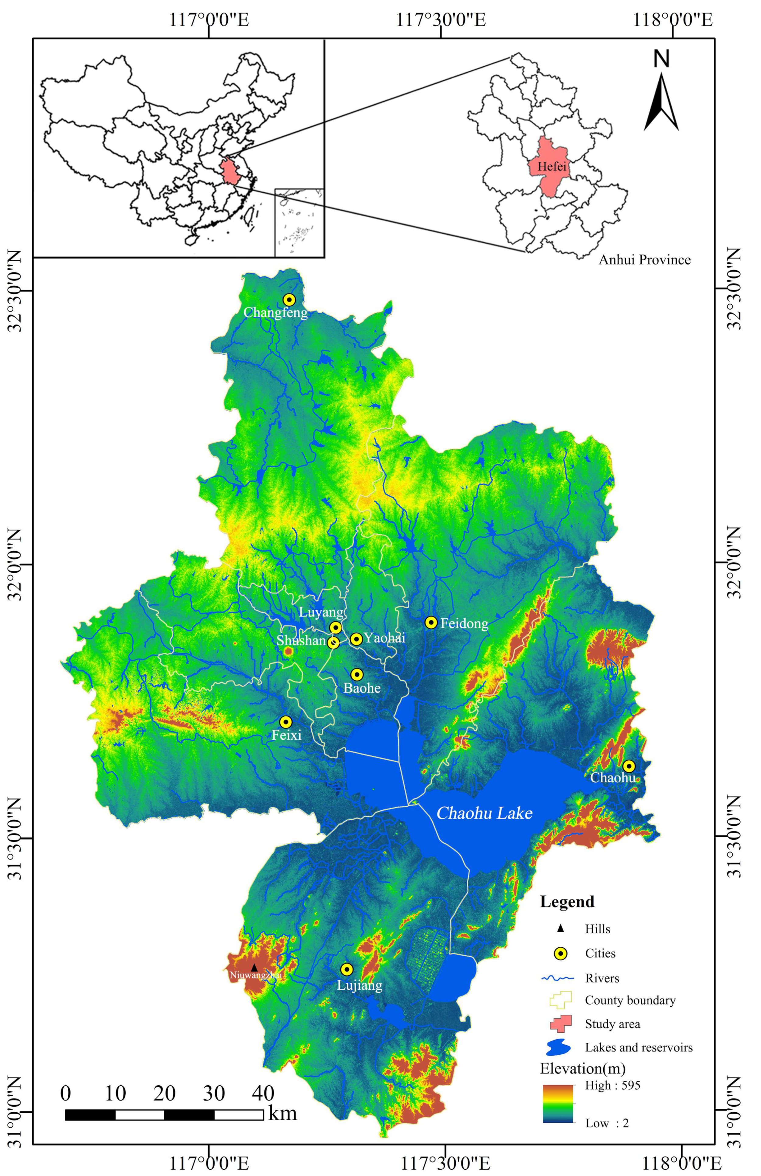
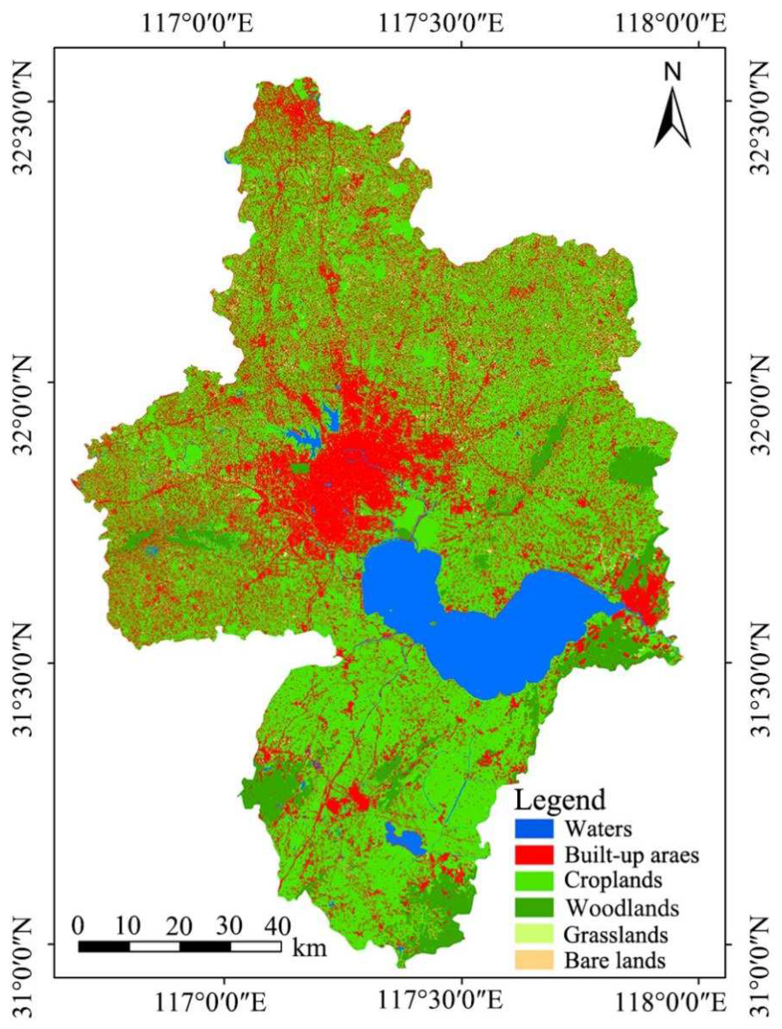
To test the reliability of the LMCM model and its superiority to other existing hybrid models, our experiment was designed as follows:
(1) Land use/cover (LUC) mapping using multitemporal Landsat images dated 2010, 2015, and 2020 and validation by ground-truth data; (2) LUCC detection, calculation of area changes and the transition matrix of each land cover type; (3) identification of LUCC drivers and constraining factors, and screening out those relevant for land use change modeling through collinearity analysis; (4) definition of the optimal units for simulation and modeling by calculating the area under the ROC curve (AUC) for each land use type at different simulation units, and using AUC as the evaluation criterion for selecting the optimal unit; (5) modeling and prediction of LUC in 2020 using the CM, LCM, MCM, and LMCM models; (6) validation of the LMCM model through a comparison of the predicted results by all these models with the classified map of 2020 to evaluate the reliability of the LMCM model and its superiority to others using Kappa coefficients; and (7) application of the LMCM model to predict LUC of 2025 based on the classified LUC maps of 2015 and 2020. The detailed technical roadmap is presented in Figure 1.

2.1. Study Area

As the capital city of Anhui Province, China, Hefei is geographically located between 116°40′ and 117°58′ E in longitude and between 30°56′ N and 32°32′ N in latitude. The total area is about 11,445 km2, including four urban districts, namely Baohe, Yaohai, Shushan, and Luyang, four counties, i.e., Feidong, Feixi, Lujiang, and Changfeng, and one municipality city (Chaohu) (Figure 2). Situated in a humid subtropical monsoon climate zone, Hefei receives an annual precipitation of about 1000 mm, whereas the average annual temperature is 15.7 °C [50,51]. The landform is mainly plains and hills, with an altitude ranging mostly from 15 to 80 m, except for Niuwangzhai hill, reaching 595 m [52].
According to the data of the seventh national census, the permanent population of the study area reached 9.37 million at the end of 2020, and the urbanization rate rose from 63.2% in 2010 to 82.28% in 2020. The proportion of the primary, secondary, and tertiary industries changed from 4.9/53.9/41.2 in 2010 to 3.3/35.6/61.1 in 2020, while the growth of GDP (gross domestic product) reached 238% in this period [53]. With the continuous adjustment of the industrial structure and rapid urbanization, the distribution pattern of land use in Hefei has also undergone tremendous changes in the past decade, causing a series of problems such as intensified man-land contradiction, environmental degradation, water pollution, and huge loss of fertile croplands. It is, hence, necessary to conduct a LUCC simulation and prediction study in this area for a better understanding of the future LUC pattern. Up to today, few studies on this topic have been reported for Hefei, and that is why we selected this city as our study area for LUCC modeling and prediction, expecting that the results of this study may provide advice to the governments for solving the above-mentioned problems.

2.2. Data Processing

As mentioned, this study involves a variety of data, including satellite remote sensing and terrain data, socioeconomic data, geographic information data, planning restriction data, and field investigation data, as shown in Table 1.

2.2.1. Data

(1) Remote Sensing data
To choose remote sensing data, two aspects must be taken into account; that is, one is cloud-free [9,54,55], and the other is the continuity of the sensor in operation [56,57]. We obtained three low cloud-cover scenes of Landsat 5 TM (19 March 2010) and Landsat 8 OLI images (1 March 2015 and 14 March 2020) with path/row number 121/38 from the USGS (United States Geological Survey, Reston, VA, USA) data server.
(2) Terrain data
The terrain data are the digital elevation model (DEM), and in total, five tiles of ASTER GDEM V3 data (30 m resolution) were acquired from NASA (National Aeronautics and Space Administration, Washington, DC, USA). Slope and aspect were derived from the DEM using a topographic modeling tool within ENVI (ENvironment for Visualizing Images).
(3) Socioeconomic data
Socioeconomic data such as population density and GDP of 2010, 2015, and 2020 were acquired from the statistical yearbooks of various districts and counties from the Hefei Bureau of Statistics.
(4) Rainfall data
The rainfall data mainly include the monthly and average annual rainfall from 2009 to 2021 recorded by weather stations in each county or district. Considering that the remote sensing images were acquired in March, we used the 6-month preacquisition rainfall data from September to February for this study.
(5) Basic geographic information data
Basic geographic data dated 2010, 2015, and 2020, mainly including the distances from highways, railways, main roads, rivers, lakes, and urban settlements, were derived from the OpenStreetMap V5.1, of which the urban settlement data were obtained from Amap V13 by writing an application programming interface (API) using java language.
(6) Planning constraint data
According to the governmental documents such as the Hefei Master Land Use Plan (2006–2020) and Master Urbanization Plan (2011–2020), the national natural reserves, the protected areas of class-1 water sources, cultural relics protection, and other factors were taken into account to delineate the prohibited areas for construction within the scope of Hefei to ensure sustainable development of the city.
(7) Field investigation data
A field survey was effectuated in the spring and summer of 2021 using OvitalMap V9.8.5, a smartphone application that allows recording not only the geographical location (GPS/Beidou) but also the survey data of each observation point. In total, 682 field LUC observation points were visited and recorded.

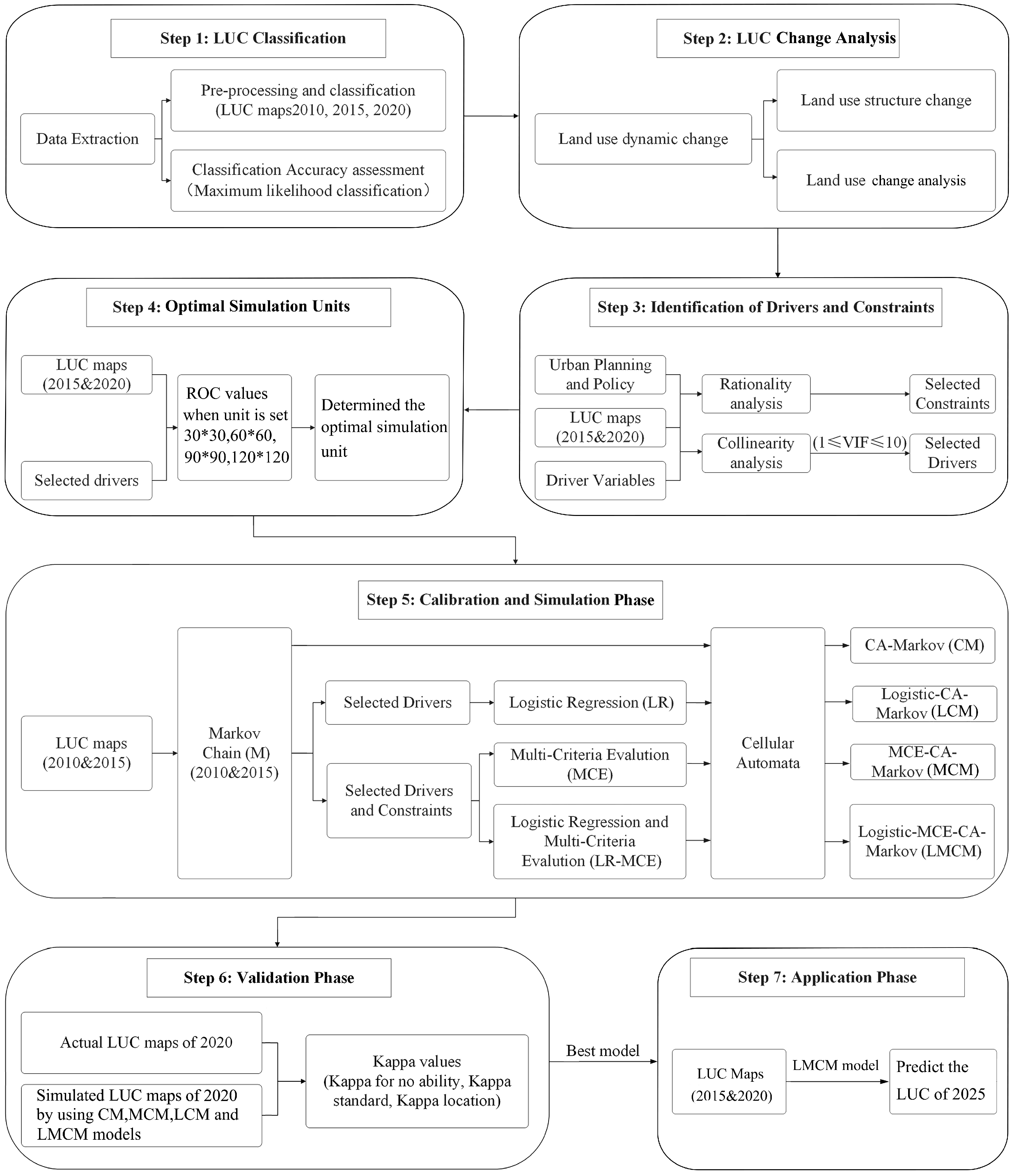
2.2.2. Processing Procedures

(1) Remote sensing data processing
Chavez (1996) found that cosine theta (θ, the solar zenith angle) is a good approximation of the upwelling transmittance from surface to sensor, and hence, the atmospheric correction approach can be simplified, and an image-based correction was proposed. Chavez (1996) called this COST (COSine Theta) model [58]. This study employed the COST model for atmospheric correction of Landsat images, in which the band minimum was used to eliminate the haze effect, and the at-satellite radiance of each band was transformed into surface reflectance [59,60]. LST (land surface temperature) was also calculated from the thermal infrared band of Landsat TM and OLI images [61,62,63,64].
Slope and aspect were produced from the DEM data and utilized as part of the environmental factors for land use classification [63]. A dataset of 13 bands, including elevation, slope, aspect, and three vegetation indices shown below, blue, green, red, near-infrared, SWIR1, SWIR2, and LST, were combined by layer-stacking function [63].
Considering the actual land cover characteristics of Hefei, three vegetation indices, namely the normalized difference vegetation index (NDVI) [65], the enhanced vegetation index (EVI) [66], and the generalized difference vegetation index (GDVI) (n = 2) [64] were employed. It is known that EVI can effectively reduce soil and atmospheric impacts [66], and GDVI is of higher sensitivity and wider dynamic range to low vegetated land covers such as bareland, urban areas, grasslands, or rangelands than other vegetation indices [64], and NDVI lies in between EVI and GDVI, a compromise of the two indices. Thus, utilization of the three indices may contribute to identifying land cover with more detail. These three vegetation indices can be obtained with the following formulae:
NDVI = ( ρ N I R ρ R ) / ( ρ N I R + ρ R )
EVI = 2.5 × ρ N I R ρ R ρ N I R + 6.0 ρ R 7.5 ρ B + 1
GDVI = ( ρ 2 N I R ρ 2 R ) / ( ρ 2 N I R + ρ 2 R )
where ρ N I R is the spectral reflectance of the near-infrared band; ρ R is that of the red band and ρ B the blue band.
(2) Factor processing
Selection of the relevant driving and constraining factors of land use in Hefei is an important step in modeling. Ten socioeconomic and geographic driving factors were selected for this purpose, i.e., population, population density, GDP and per capita GDP, and urbanization rate from 2010 to 2020, which were all interpolated using the inverse distance weighting (IDW) approach. This method mainly applies larger weights to observations closer to the target point and smaller weights to observations farther away from the target point in order to predict spatial positions that have not yet been observed. Though Milillo and Gardella (2008) found that ordinary kriging is more accurate than IDW in retention of original image features [67], Spokas et al. (2003) and Gong et al. (2014) have shown that IDW is superior to kriging in the estimation of landfill methane flux [68] and groundwater arsenic concentrations [69] whereas Munyati and Sinthumule (2021) found that for the forest, kriging has a higher correlation of tree density with NDVI than IDW while for woodlands, IDW has a higher correlation than kriging in estimating tree density [70]. Thus, whether kriging or IDW interpolation performs better is case-dependent. For simplicity, we selected IDW for the interpolation of these factors.
Geographical factors, including elevation, slope, and distances from the main roads, highways, railways, rivers, reservoirs, and urban settlements, were obtained by Euclidean distance analysis. In addition, four constraining factors were identified as well, and they are the protected farmland area, the first-class protected water source area, the core area of the scenic spot, and the main urban area. The constraining factors are in Boolean, set either 0 or 1, where “0” means the forbidden area for development, and “1” represents the developable ones.
To match the Landsat and DEM data, all factors were resampled to 30 m in resolution within datum WGS 84 and projection UTM Zone 50N and kept in the same dimension (same row and column number).

2.3. Methods

2.3.1. LUC Mapping and Its Dynamic Changes

Mapping LUC is one of the important components of LUCC modeling. Based on the third national land survey in combination with field investigation, we defined 21 initial categories of the ground-truth samples (regions of interest, ROIs) for the study area, half of which was employed for training, i.e., the training set (TS) and the remaining half for verification, or more precisely, the verification set (VS). The maximum likelihood algorithm was applied to the 13-band datasets for supervised classification, with the TS for training and the VS for verification of the classified maps. In order to facilitate further research, all the initial classes are merged into six main categories according to their similarity, namely, waters, built-up areas, croplands, grasslands, barelands, and woodlands, including local patches of forests and shrublands (Table 2). Accuracy evaluation was performed by confusion matrix, and the main indicators are overall accuracy (OA), Kappa coefficient (KC), producer accuracy (PA), and user accuracy (UA).
After classification, different LUC types and their spatial distribution of each observed year (2010, 2015, and 2020) were quantified, and their change trends were analyzed.

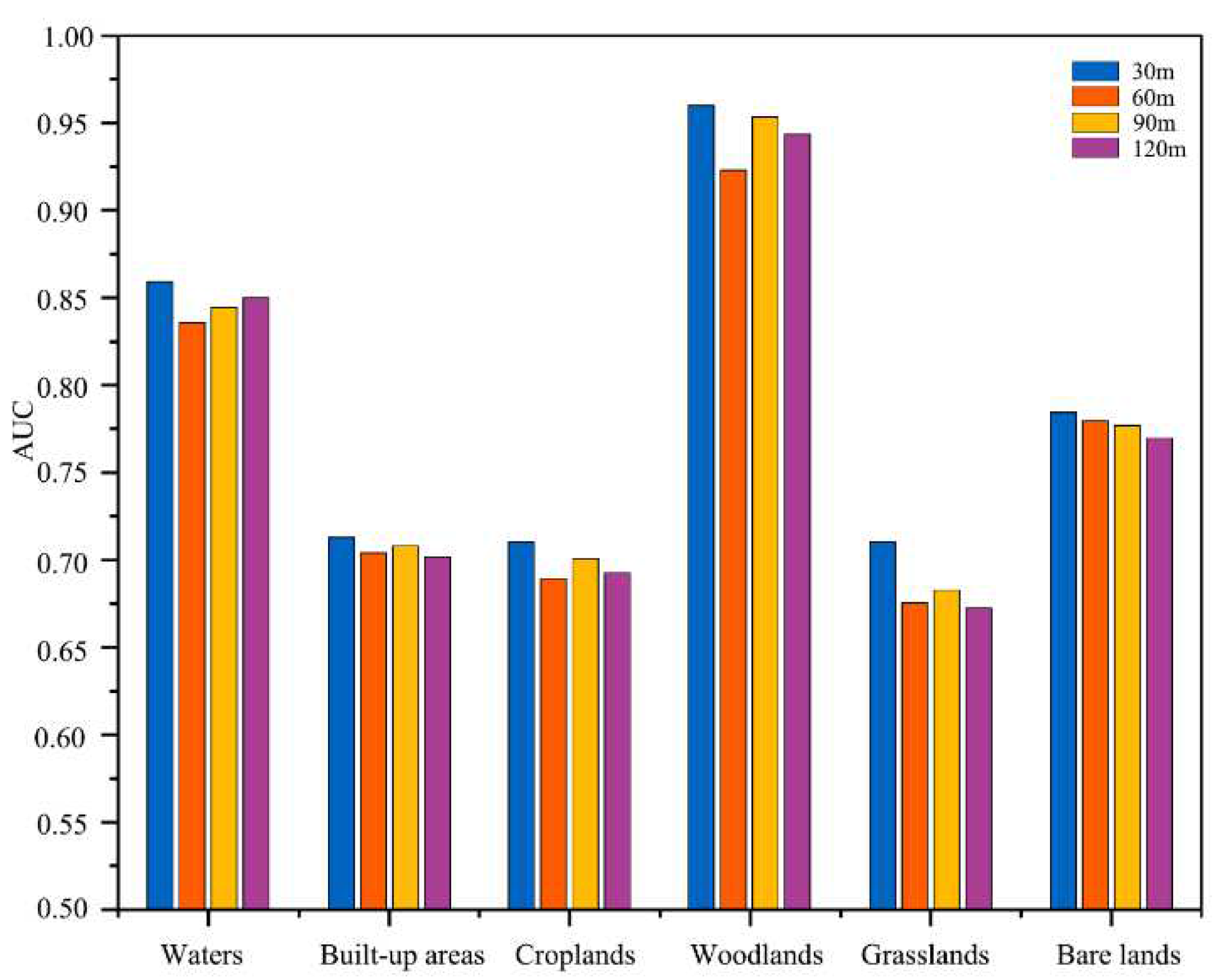
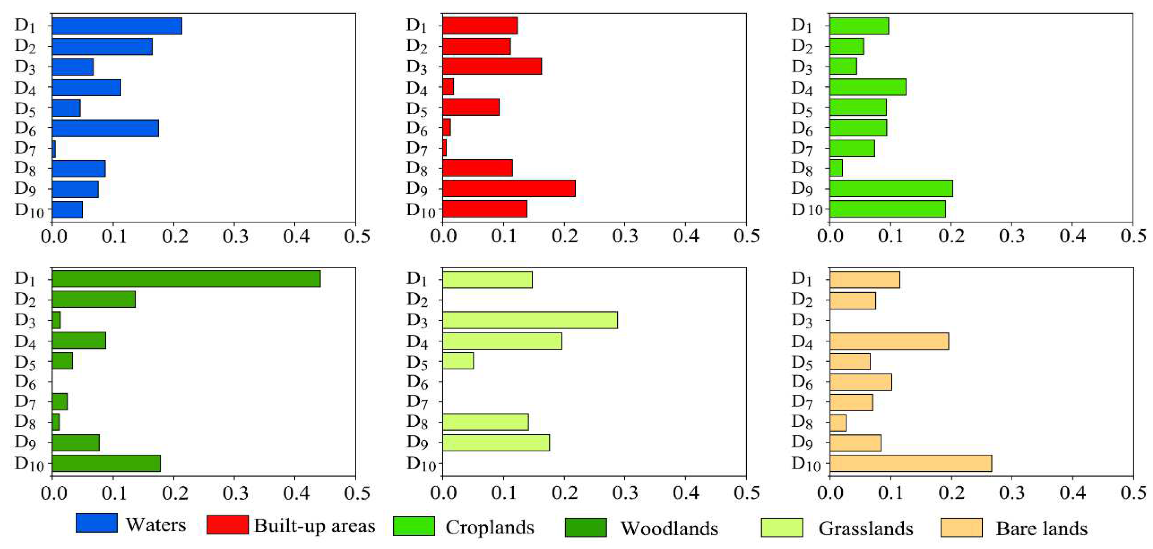
2.3.2. Determination of the Driving Factors and Optimal Simulation Units

To reduce spatial dependence and ensure adequate sample size, this study adopted an approach by combining systematic sampling of land use data and driving factors (25 grid intervals) with random sampling (additional 5%).
(1) Driving factors
Before LUCC modeling, it is critical to eliminate the multicollinearity of the driving factors. The multicollinearity diagnosis was effectuated by the tolerance (TOL) and the variance inflation factor (VIF), which are reciprocal to each other. When the VIF falls between 0 and 10, there exists no collinearity among the factors, but when the VIF > 10, it implies a collinearity exists among the factors [71]. Our test revealed that the VIF of almost all variables is < 10 except rainfall and temperature, and thus, these two factors were removed for further analysis. There is no collinearity or inter-dependency among the remaining factors (Table 3 and Table 4).
(2) Best simulation unit
The factors, mechanisms, and characteristics of land use change in space may arise differently if simulation is conducted at different unit sizes, and it is necessary to select an appropriate simulation unit size for this purpose. Considering the actual surface area in this study and the requirements for accuracy, four simulation units (cell size) were proposed for the test: 30 × 30 m2, 60 × 60 m2, 90 × 90 m2, and 120 × 120 m2. Logistic regression analysis was used for this optimal analysis, where the results were tested by using the receiver operating characteristic (ROC) approach developed by Pontius and Schneider (2001). The area under the ROC curve (AUC) of each land use type with different simulation units was calculated, and the AUC was regarded as the evaluation criterion for the selection of the best unit. Usually, the AUC value comes between 0.5 and 1, and when 0.5 ≤ AUC < 0.7, the accuracy of the prediction result is low; when 0.7 ≤ AUC < 0.9, indicating a medium precision, and when 0.9 ≤ AUC < 1.0, it means a high precision [72].

2.3.3. Simulation and Validation

(1) Characters of the different hybrid models and simulation
The CM model is a combination of CA with the Markov model, in which the latter is a stochastic model that allows us to obtain the transition matrices of LUC from one state to another [73,74,75]. The transition equation for land use status is shown as follows:
S ( t + 1 ) = P i j S ( t )
where S is land use states, t , t + 1 are the observed time points, and P i j is the probability matrix of state transition and is expressed as follows:
P i j = P 11 P 1 n P n 1 P n n
where 0 ≤ P i j < 1 and j = 1 n P i j = 1 ( i , j = 1, 2, , n ); n is the land use type number. The disadvantage of this kind of model lies in that it provides neither information of precise spatial location nor driving forces [76].
CA are discrete models regarded as spatiotemporal dynamic systems based on local rules [77,78], determined by a series of rules constructed by the model, and the core part is the definition of transformation rules [79]. The three main characteristics of CA are parallelism, consistency, and locality, which provide great help in dealing with complex and ever-changing geographic systems and demonstrate strong adaptability to geographic systems. CA systems usually include five components: cell, cell space, cell neighbors, transformation rules, and transformation time. The formula is demonstrated as follows:
S ( t + 1 ) = f S ( t ) , N
where S is a set of states of the finite cells; f is the transformation rule of local space; t and t + 1 are different moments of time; and N is the neighborhood of cells.
The prediction of land use change using the Markov model is mainly a quantitative prediction, which cannot predict the spatial distribution of different land types in the study area. However, the CA model has the concept of spatial information and the ability to simulate dynamic evolution. Therefore, the CM model takes advantage of both the Markov chain and CA models and may lead to a better spatiotemporal prediction of land use change.
The LCM model is mainly based on the LR and CM models. The LR model has been widely used in the prediction of land use change [80] and natural disaster (e.g., landslide) risk assessment [81,82]. The LR model is a binary logistic regression (BLR) relationship formed between a dependent variable and multiple independent variables to predict the probability of an event occurring in a certain region. Its advantage is that the independent variables can be continuous or discrete [83]. In this study, a certain land use type, such as croplands, grasslands, etc., was treated as the dependent variable, and the corresponding grid attribute was assigned a value of 1; on the other hand, the driving factors, such as elevation and population density, serve as independent variables. The equation of the BLR model is shown as follows:
logit ( P i ) = ln P i 1 P i = β 0 + β 1 X 1 + β 2 X 2 + + β n X n
where P i is the probability that land use type i may appear in the given pixel;   X n is the influencing or driving factors; β 0 is a constant; and β n is the partial regression coefficient of the corresponding factor Xn.
The MCM model is a combination of MCE and CM. The MCE model is an analytical method that evaluates a series of unrelated influencing factors in order to provide optimal decision-making. The core of the MCE model is to establish corresponding standards for different land types and then provide a reference for decision-making by analyzing the factors that affect different land types. MCE involves two types of influencing factors, namely the constraining and the driving factors. The constraining factor is to maintain the current status of areas that do not undergo land type conversion within the observation year, which is closer to the actual situation, takes dichotomous values of either “0” or “1”, and there is no intermediate gray area [84]. Among them, ‘0’ represents areas that are prohibited from development, and ‘1’ represents areas that can be developed. This is a hard decision and does not require standardized processing in later land use change modeling. The driving factor represents the degree to which a certain land use type is suitable for development, which refers to the factors that will affect the mutual conversion between different land types during the observation year. Different factors will have different impacts on the conversion results. In the process of creating the suitability atlas, we used the fuzzy membership function to control points for normalization of the influencing factors to a continuous value ranging from 0 to 255, which belongs to soft decision-making. Finally, the weights of all factors are determined by the analytic hierarchy process (AHP), and each standardized factor is integrated with its corresponding weights and superimposed on the constraining factor by the weighted linear combination (WLC) approach, and the suitability distribution map of each local class is obtained as a supplement to the local rules of CA. The equation for the MCE model is shown as follows:
S = w i x i c j
where S is the score of suitability as a combination of all selected factors; w i is the weight of the observed driving factor i; x i is the score assigned to the observed driving factor i; and c j is the value of the selected constraining factor j.
The LMCM model, as mentioned earlier, is composed of LR, MCE, CA, and Markov models, taking advantage of all these different models but avoiding their disadvantages. The LMCM model places more emphasis on the inherent characteristics of the sample data, making it more accurate in simulating and predicting land use changes. The fully standardized logistic regression coefficient was proposed by American scholar Scott Menard in 1995 [85]. Unlike other standardized regression coefficients, it not only considers the standardization of independent variables but also the standardization of dependent variables.
Firstly, through the logistic regression and linear regression models, the significance, nonstandardized regression coefficient, standard deviation, and other parameters were obtained, and then, according to the approach proposed by Menard (1995) [85], the fully standardized LR coefficient was calculated in terms of Equation (9):
γ m   =   c ( S X ) R / S l o g i t ( Y ^ )
where γ m is the fully standardized LR coefficient; c is the unstandardized LR coefficient; S X is the standard deviation of the driving factor X; S l o g i t ( Y ^ ) is the standard deviation of logit(Ŷ), i.e., the standard deviation of the predicted values of logit(Y); and R is the correlation coefficient between the observed values of Y (either 0 or 1) and the predicted values of Y (predicted probabilities for each type). Equation (9) provides information on the importance of each driving factor.
The logistic regression coefficient with a significance level of greater than 0.05 was excluded, and the remaining one was retained for weight calculation:
w m = | γ m | γ 1 + γ 2 + + | γ n |
where w m is the normalized regression coefficient with the driving factor m;   γ m is the fully standardized LR coefficient; and γ n is the normalized regression coefficient value for the last driving factor after screening, 1 ≤ mn.
After obtaining the weight values ( w m ) of the driving factors of each land use type, the probability of land use type in each raster cell was determined by the WLC in the MCE model, and then LUCC prediction was obtained by the collection editor.
In the simulation process, the constraints on the conversion rules were divided into two groups, i.e., mandatory and ordinary. The mandatory constraints were used as constraining factors, and the ordinary constraints were used as driving factors. The processing methods of the two groups of constraints are different, and the collinearity analysis of the driving factors allows for reducing their spatial autocorrelation and thereby minimizing the interference of data errors on the simulation accuracy. Furthermore, in the test of all the models through linear regression and LR analyses with a significance level of < 0.05, a fully standardized LR coefficient was obtained and converted into the weight value (or probability) of each driving factor. The latter, which defined the weight value, was combined with the constraining factor through the WLC approach in the MCE model. Then, the CM model was harnessed for land use modeling where adjustment of parameters by expert experience or knowledge was avoided.
(2) Validation phase
The performance of the above models was evaluated using the Kappa coefficients or indices, which include Kappa for no information (Kno ) , Kappa standard (Kstandard), and Kappa location (Klocation) [86]. Kappa indices usually come between 0 and 1, and when they are less than 0.5, it indicates that the consistency is not satisfactory; when they come between 0.5 and 0.75, it is a moderate degree of consistency; when they are equal to or greater than 0.75 but less than 1, it represents a high degree of consistency; and when Kappa indices = 1, it implies a complete consistency.
K n o = (   P 0 NQNL ) / ( 1 NQNL )
K s t a n d a r d = ( P 0 MQNL ) / ( 1 MQNL )
K l o c a t i o n = ( P 0 MQNL ) / ( MQPL MQNL )
where P 0 is the proportion of correct classification; NQNL is neither quantitative nor location information; MQNL is the ability to maintain a medium amount of information but no ability to maintain location information; and MQPL is the ability to maintain a medium amount of information but also has the ability to perfectly maintain location information.
In addition, to evaluate the rationality of LUC mapping and simulation, especially the prediction of waters, the mean standard deviation classification method [87] was applied to establish a weighted Markov chain model to estimate the 6-month rainfall from September 2024 to February 2025 using the monthly precipitation data from 2009 to 2021 as reference.

3. Results

3.1. Classification and LUCC

3.1.1. LUC Maps

In terms of the above procedures, LUC maps of 2010, 2015, and 2020 were obtained and presented in Figure 3. The classification accuracy was evaluated in two ways: One was using the VS to calculate, through the confusion matrices, in which the OA, PA, and UA are all above 96%, and the KC is above 0.93 (Table 5, see Appendix A for the confusion matrices). The other was to use the 682 field observation points (samples) obtained in the summer of 2021 to verify the classified map of 2020, and the observation accuracy is greater than 95%. These show that our classified land use maps are of high accuracy and reliability and can be used for LUCC modeling.

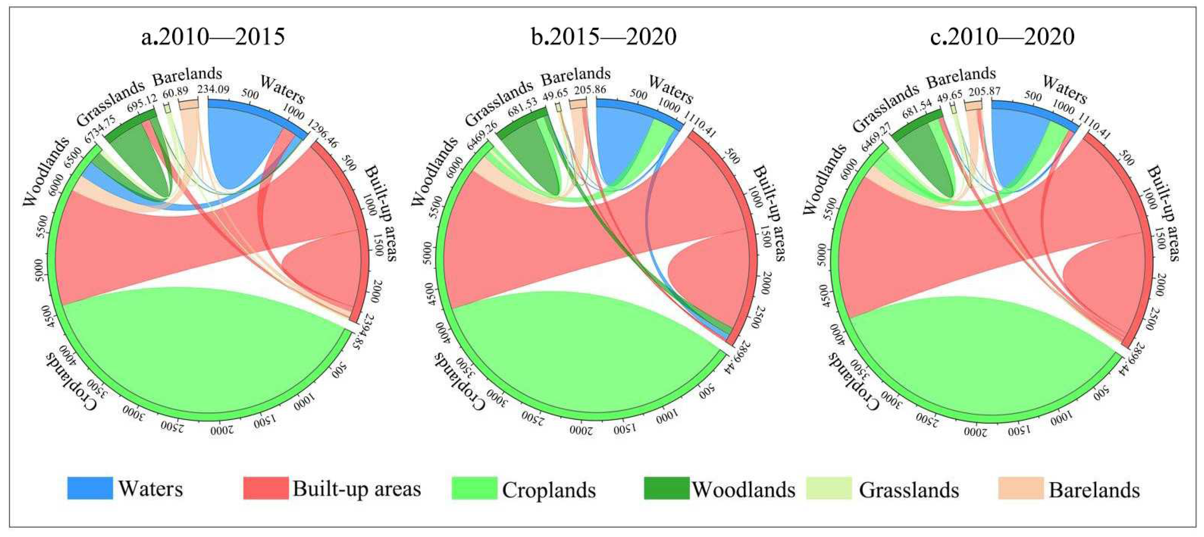
3.1.2. Changes in Land Use

LUC types, areas, and their percentages of the three observation years are shown in Table 6, and the mutual conversion of different land use types is presented in Figure 4. We see that the most important land use type from 2010 to 2020 is croplands, accounting for 61.65%, 58.99%, and 56.67%, respectively. During this period, croplands had been decreasing at an annual rate of 0.49%, with a total reduction of 568.14 km2, in which croplands were converted into built-up areas, waters, and forests/woodlands. Woodlands, grasslands, and barelands also appear to have a decrease, but the rate of reduction was relatively moderate. Built-up areas are the only land use type that had been continuously increasing by 804.69 km2 in surface area from 2010 to 2020, mainly converted from croplands, partially from waters, grassland, and barelands (Figure 4). Different from the other LUC types, waters showed a variation in surface area in the observed period, more concretely, gained an increase in 2010–2015 and then experienced a decrease in 2015–2020. The details of mutual conversion and net change among the different land use types can be checked in the Sinogram (Figure 4).

3.2. Simulation Factors and the Optimal Simulation Unit

The ten driving factors with a VIF < 10 and four constraining factors used for simulation were mapped and are presented in Figure 5.
Corresponding to different modeling units, i.e., 30 m, 60 m, 90 m, and 120 m, respectively, their AUC values of the modeling results, or rather, the predicted LUC maps versus (vs.) the VS were calculated and shown in Figure 6. It was found that the AUC values of various types of land cover are best when the modeling unit is 30 m. Hence, all the results were produced when the simulation unit was set to 30 m. Here, woodlands reached the highest fitting, 0.96, among all the LUC types.

3.3. Simulation Results and Accuracy Evaluation

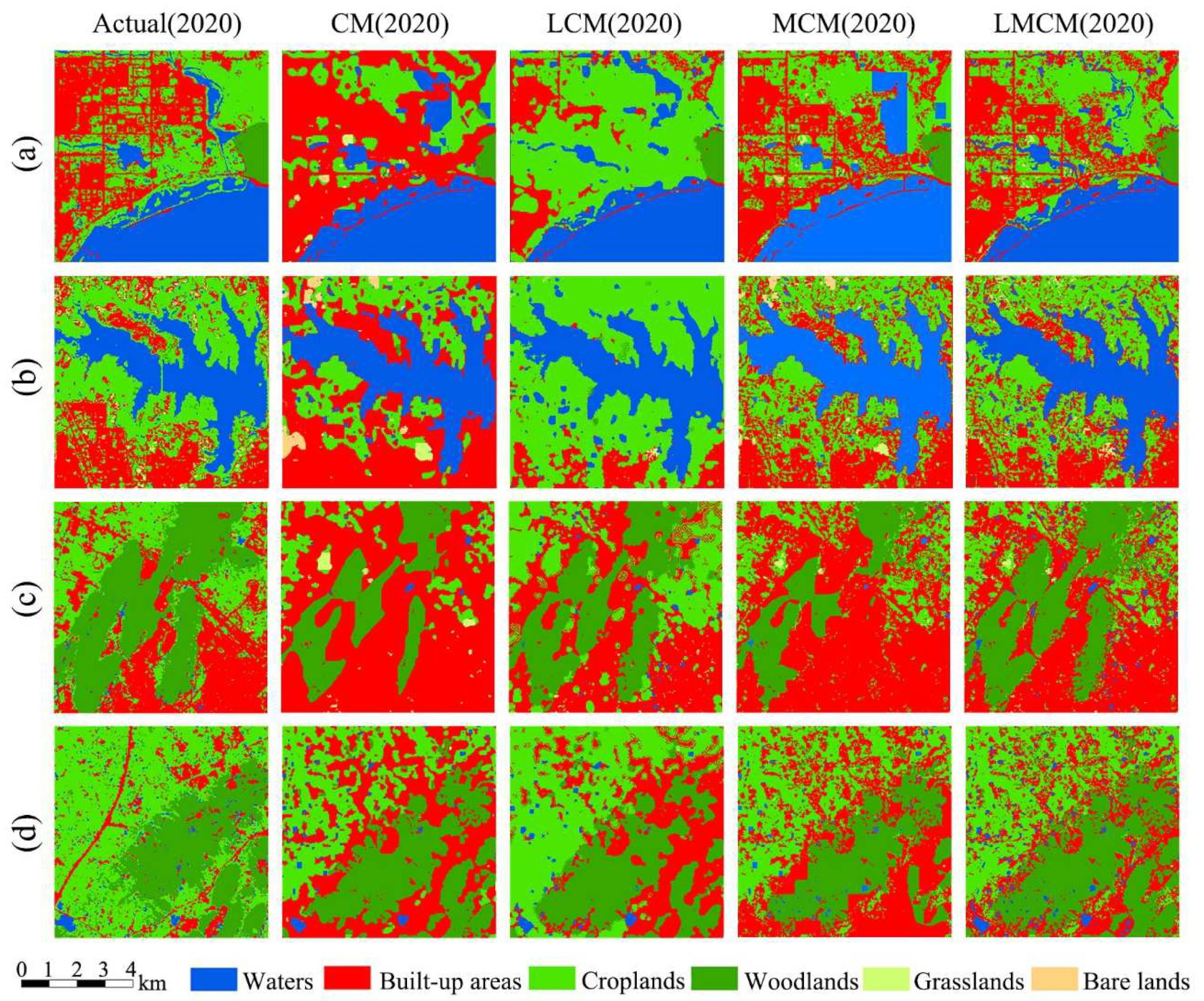
3.3.1. Simulation Results of Different Models

Based on Equation (10), we obtained Figure 7, indicating the driving factors for different land use. As for the built-up areas, the population density (D9), distance to roads (D3), elevation (D1), and average GDP per unit land (D10) are the socioeconomic and spatial determinants, while croplands are associated with the population density (D9), average GDP per unit land (D10), distance to motorways (D4), and elevation (D1). For waters, distances to lakes/reservoirs (D6), elevation (D1), and slope (D2) are the most important physical determinants, accounting for 55.4%; whereas elevation (D1), slope (D2), and average GDP per unit land (D10) have the strongest impact on woodlands, including forests and shrublands, taking up 44%, which is in line with the ground-truth observation in field; and grasslands are susceptible to the influence of neighborhood, i.e., distance to roads (D3).
The simulated 2020 LUC maps were obtained from different modeling (Figure 8). As we can see in Figure 8, the LCM model is quite different from the other three, and the most intuitive is that the spatial distribution of the built-up areas is more concentrated than the mapped one using remote sensing data. The CM and MCM models have produced similar results but overestimated barelands. The LMCM model performed well in a simulation of different LUC types, especially built-up areas and barelands, in comparison with the classified LUC map of 2020.
In order to better display the effect of different models, four representative zooms were selected for a detailed insight and comparison of the models (Figure 9). In Zoom (a), it is seen that the simulation effect of CM and LCM models is not as good as LMCM. Zoom (b) reveals that the MCM model is able to simulate correctly the built-up areas as grasslands and barelands, similar to LMCM. Zoom (c) exhibits that the LMCM model has a good performance in the simulation of woodlands and a better effect than other models. Zoom (d) shows that the above models cannot simulate the impacts of policy-driven change, such as newly constructed highways, in the realistic land use in 2020.

3.3.2. Accuracy Comparison

Table 7 demonstrates that LUC prediction by the LMCM model performed better (with higher Kno, Kstandard, and Klocation) than others. Kno and Klocation are 0.8106 and 0.8025, respectively, 2.14%–6.63% higher than those of other models, indicating a better simulation effect of the new hybrid LMCM model than others in terms of location and quantity.

3.4. Predicted Land Use Pattern of 2025

Taking the LUC maps of Hefei in 2015 and 2020 as the benchmark, combined with the driving and constraining factors, the LMCM model was employed to predict the land use pattern of Hefei in 2025, and the final LUC map of 2025 obtained is presented in Figure 10. Table 8 shows that all six land use types would experience varying degrees of change from 2020 to 2025. Compared with 2020, built-up areas, grasslands, and barelands are likely to have an increasing trend, among which the increase in built-up areas is the most evident, amounting to 443.39 km2, which shall be the most significant change in the next five years, with an annual growth of 88.68 km2. Waters, croplands, and woodlands are likely to have a decreasing trend during this period. Among them, croplands would decrease the most, reaching 294.14 km2, with an annual decrease of 58.83 km2, followed by waters, with a decrease of 159.67 km2, with an annual reduction of 31.93 km2.

4. Discussion

4.1. LUC Detection, Prediction, and Their Driving Forces

As the above change detection and simulation revealed, the net increase in built-up areas was 804.69 km2 in 2010–2020, but this expansion will continue and may reach 3342.83 km2 in 2025, with an increase of 443.39 km2 from 2020 to 2025 (Table 6 and Table 8). This increase shall be associated with urban extension, or rather, urbanization driven by population growth and different policies [88,89,90,91], as the demand for residential, transportation, commercial, medical health, and other construction has been increasing, resulting in the rapid expansion of built-up areas.
A net decrease of 568.14 km2 in croplands was detected in the period 2010–2020, and this may continue and decline by 294.14 km2 from 2020 to 2025. Croplands are a key land use for food production; nevertheless, a substantial part of croplands has been converted into built-up areas in the past decades (Figure 4) [88,89,90,91]. To meet the demand of food production and security in the context of a growing population, it is essential to compensate for the loss of croplands due to urbanization, and hence, reclamation has been effectuated in grasslands and woodlands/forests via slash-and-burn procedure in the past decades [88]. But as a whole, the conversion of croplands into built-up areas seems faster than reclamation, leading to a continuous decrease in the former.
Though the variation in the water looks different from other land use, an increase of 56.33 km2 from 2010 to 2015, followed by a decrease of 186.08 km2 from 2015 to 2020 (Table 6), may be partially related to the conversion of the waters into built-up areas because of the more rapid urbanization in 2015–2020 (504.58 km2) than in 2010–2015 (300.11 km2). Another reason for this variation is the fluctuation in rainfall. We calculated the 6-month preacquisition rainfall from September to February and found that they were, respectively, 362.97 mm, 448.06 mm, and 283.21 mm in 2009–2010, 2014–2015, and 2019–2020 (see Appendix B). Thus, the variation in water surface may be a consequence of both urbanization and changes in rainfall. As the LUCC simulation revealed, the surface of waters in 2025 is likely to be 950.73 km2, indicating a decrease in waters from 2020 to 2025. This can be an integrative result of urbanization and possible rainfall reduction, the same as the period 2010–2020. As we have modeled, the 6-month rainfall from September 2024 to February 2025 is likely to be 237.57 mm–310.60 mm with a mean of 274.09 mm, slightly lower than that of 2019–2020. The prediction of waters of 2025 using the LMCM model, a reduction of 159.68 km2 from that of 2020, seems reasonable.
LUCC is mainly due to the combined action of natural and human driving factors. The effect of natural factors on LUCC is lasting and profound, and it is the controlling factor of the macro-LUC pattern. Landform and climate are the main natural factors influencing LUCC. The landform of Hefei is generally declined in the southeast and northwest, relatively flat in the middle and north, and hilly in the southeast. The river system is well developed, including the Chaohu Lake, and thus, the LUC types, such as built-up areas, woodlands, and croplands, are obviously distributed in space, taking the topographic advantages. For example, built-up areas and croplands are concentrated in flat terrain, while grassland and forests are mostly distributed in places with large undulations and relatively high altitudes.
The impacts of human factors on LUCC are active and significant, e.g., the implementation of the “New Urbanization Plan of Anhui Province (2016–2025)” emphasizes urbanization as the core growth of Hefei and makes the regional central city bigger and stronger. The strategy to “Develop Strong and Big Capital” puts economic development superior to others and has led to the transformation of a large amount of croplands, waters, and forests into built-up areas (Anhui Government, http://fzggw.ah.gov.cn, accessed on 1 July 2021).
In short, the impacts of human activities on LUC are increasing, and it is urgent to adopt relevant policies and measures to rationally plan land use in space and to make the disorderly expansion of cities in order.

4.2. Performance of Different Models

As presented in Table 9, the previously published models and their combinations expose disadvantages, whereas the one we proposed avoids these shortcomings. We noted that the driving and constraining factors do not take part in the simulation of the CM model, and the LCM model does not incorporate the constraining factors in this process either. Although the MCM model involves driving and constraining factors, the disadvantage lies in its dependence on expert knowledge, which increases the uncertainty of simulation. However, the proposed LMCM model does not rely on expert knowledge and is able to combine both driving and constraining factors to effectuate land use simulation based on local conditions and may achieve a better land use prediction where rapid socioeconomic development has been taking place.
Through the comparison of simulation results, we found that the MCM model is superior to the LCM and CM models, and this is consistent with the previous research by other authors. Nevertheless, as we can see in Table 9 and Figure 8 and Figure 9, the LMCM model performs even better than MCM and the other two hybrid models as its Kstandard is 2.14–6.63% higher than the latter three. Moreover, the LMCM model has a better simulation effect in built-up areas, waters, and woodlands/forests. These indicate an improvement of the LMCM model in terms of simulation accuracy over the others.
However, attention should also be paid to the prediction errors of different LUC types, such as newly built railways, new urbanization, and lake reclamation for farming or urbanization. There may be other measures in the predicted year 2025, which should be further studied in conjunction with policy promulgation to improve the reliability of the simulation and prediction.

4.3. Reproducibility, Limitations, and Future Work

As mentioned, the proposed methods, including the required materials and procedures, allow the development of the new hybrid LMCM model and its application in LUCC simulation to predict future land use/cover patterns. The approaches are, hence, reproducible, and the new model is applicable elsewhere for a similar purpose.
During this research, some problems were also encountered. Although the proposed LMCM model has led to a good simulation of LUCC, better than other models, the impact of policy implementation and some pandemics and natural disasters such as COVID-19 and earthquakes have not been integrated into the simulation due to the difficulty of quantification of these factors. This is expected to be sorted out in future work.
There may exist uncertainty in the predicted LUC of 2025 as the real LUC situation in the future may be much more complex, and land use change may not exactly occur as we have simulated. Therefore, further research should include the following solutions: (a) Higher resolution remote sensing data should be used to obtain more precise LUC maps with higher accuracy and reliability. (b) For cities with similar policy implementation, urban development trends, and urbanization stages, more data on policy implementation in space and time should be integrated for modeling to help design a more realistic land use simulation model for advising sustainable land management.

5. Conclusions

Based on the field observation and LUC mapping by remote sensing, this paper proposed a new hybrid model LMCM for LUCC simulation, or rather, prediction of the future LUC pattern. The novelty lies in that the new LMCM model is able to combine both the driving and constraining factors without dependence on expert knowledge and perform better LUCC simulation and prediction than other models, e.g., CM, LCM, and MCM, in terms of three indicators, Kno, Kstandard, and Klocation. Our test demonstrated that these three indicators of the LMCM model are higher by 1.72–5.4%, 2.14–6.63%, and 2.78–9.33%, respectively, than CM, LCM, and MCM models. Moreover, the fully standardized logistic regression coefficients were used as a weight link for model development for the first time, and this can be regarded as a prototype for future model development. The predicted LUC pattern of 2025 in Hefei may provide a crucial reference to the governments for their policy-making as the predicted reduction in croplands, waters, and forests is likely to become a heavy burden or even an overburden to ecological resources. Thus, our study may help the implementation of different policies such as “Division of the Ecological Function in Anhui” and “Integrated Urban Planning of Hefei” as the obtained results may provide pertinent advice for optimization of land use and resource allocation in different domains. In addition, taking advantage of the LMCM model, we would suggest extending the study to provincial and even national scales for simulating LUCC in the future. This is likely to be the added value of the study in guiding urban planning and spatial planning of territory not only in Hefei but also in the whole province and even in the whole country. The model can also be applied to other areas of the world for the same purpose.
However, there are still some shortcomings in the research process of this article; for example, the driving and constraining factors selected in this study are still not comprehensive enough, which will, to some extent, affect the accuracy of LUCC simulation and prediction. Although the LMCM hybrid model performs better than other models in LUCC simulation, it still faces uncertainties in the simulation process due to unforeseeable factors such as policy implementation. We hope to address these issues in future work.

Author Contributions

Conceptualization, Y.H. and W.W.; methodology, Y.H.; software, Y.H., X.X., X.K., Y.S., Y.L. and R.J.; validation, Y.H., W.W., X.X., C.M., M.X., S.L., A.L., X.S. and A.C.; formal analysis, X.X., X.K., Y.S., C.Z., W.L., Y.L., R.J. and P.S.; investigation, Y.H.; W.W., L.F. and X.X.; resources, W.W.; data curation, Y.H. and X.X.; writing—original draft preparation, Y.H.; writing—review and editing, W.W.; visualization, Y.H.; supervision, W.W.; project administration, W.W.; funding acquisition, W.W. All authors have read and agreed to the published version of the manuscript.

Funding

This research was funded by the Start-up Fund for Scientific Research of the East China University of Technology (No: DHTP2018001) and the Jiangxi Talent Program (No: 900/2120800004), both granted to W.W. and the APC was funded by W.W.

Data Availability Statement

The datasets used and/or analyzed during the current study are available from the corresponding author upon reasonable request.

Acknowledgments

Landsat images were obtained freely from the USGS data server (glovis.usgs.gov, accessed on 1 April 2022), and ASTGTMV003 (30 m) data from NASA (www.earthdata.nasa.gov, accessed on 10 April 2022).

Conflicts of Interest

The authors declare no conflict of interest.

Abbreviations

IGBPInternational Geosphere-Biosphere Programme
IHDPInternational Human Dimensions Programme on GlobalEnvironmental Change
LUCCLand Use/Cover Change
CACellular automata
CMCA–Markov
LCMLogistic–cellular automata–markov
LRLogistic regression
BLRBinary logistic regression
MCEMulticriteria evaluation
MCMMCE–CA–Markov
LMCMLogistic–multi-criteria evaluation–cellular automata–markov
LUCLand use/cover
USGSUnited States Geological Survey
DEMDigital elevation model
NASANational Aeronautics and Space Administration
GDPGross domestic product
APIApplication programming interface
COSTCosine function of the solar zenith angle (theta)
LSTLand surface temperature
NDVINormalized difference vegetation index
EVIEnhanced vegetation index
GDVIGeneralized difference vegetation index
IDWInverse distance weight
WGS84World Geodetic System 1984
UTMUniversal Transverse Mercator grid system
ROIsRegions of interests
TSTraining set
VSVerification set
OAOverall accuracy
KCKappa coefficient
PAProducer accuracy
UAUser accuracy
TOLTolerance
VIFVariance inflation factor
ROCReceiver operating characteristic
AUCArea under the ROC Curve
AHPAnalytic hierarchy process
WLCWeighted linear combination
KnoKappa for no information
KstandardKappa standard
KlocationKappa location
AIArtificial intelligence

Appendix A. Confusion Matrices of Land Use/Cover Mapping Dated 2010, 2015, and 2020

Table A1. Mapping of 2010, overall accuracy = (42,745/44,358) 96.3637%, Kappa coefficient = 0.9329.
ClassProducer Accuracy
(Percent)
User Accuracy
(Percent)
Producer Accuracy
(Pixels)
User Accuracy
(Pixels)
Waters93.2096.511356/14551356/1405
Built-up areas98.7995.131386/14031386/1457
Croplands99.8291.4115,527/15,55515,527/16,987
Woodlands94.4599.9615,527/25,88724,450/24,459
Grasslands45.1636.8414/3114/38
Barelands44.44100.0012/2712/12
Table A2. Mapping of 2015, overall accuracy = (50,989/51,684) 98.6553%, Kappa coefficient = 0.9733.
ClassProducer Accuracy
(Percent)
User Accuracy
(Percent)
Producer Accuracy
(Pixels)
User Accuracy
(Pixels)
Waters98.8398.26678/686678/690
Built-up areas99.5991.203847/38633847/4218
Croplands99.1097.6312,879/12,99612,879/13,191
Woodlands99.04100.0033,551/33,87633,551/33,551
Grasslands34.69100.0031/9834/34
Barelands0.000.000/1650/0
Table A3. Mapping of 2020, overall accuracy = (35,217/36,057) 97.6704%, Kappa coefficient = 0.9566.
ClassProducer Accuracy
(Percent)
User Accuracy
(Percent)
Producer Accuracy
(Pixels)
User Accuracy
(Pixels)
Waters69.7198.891335/19151335/1350
Built-up areas99.5994.291469/14751469/1558
Croplands99.9293.4610,436/10,44410,436/11,166
Woodlands99.1499.9821,822/22,01121,822/21,827
Grasslands51.1697.7844/8644/45
Barelands88.10100.00111/126111/111

Appendix B

Table A4. Rainfall Data from 2009 to 2021.
YearAnnual Rainfall (mm)Rainfall from September to February (mm)
20091099.82362.97
20101430.02372.87
20111048.77209.80
20121037.34352.30
20131043.43271.02
20141303.27448.06
20151386.33324.36
20161658.11667.51
20171058.93390.14
20181772.41570.23
2019651.00283.21
20201530.60359.67
20211194.82279.15

Appendix C

Figure A1. Corresponding Table of Land Types and Colors.
Land 12 01899 g0a1

References

  1. Turner, B.L.; Skole, D.L.; Sanderson, S.; Fischer, G.; Fresco, L.; Leemans, R. Land-Use and Land-Cover Change, Science/Research Plan, Global Change Report; IIASA: Stockholm, Sweden; Geneva, Switzerland, 1995. [Google Scholar]
  2. Lambin, E.F. Land-Use and Land-Cover Change (LUCC)—Implementation Strategy; IGBP Report No. 48 and HDP Report No. 10. Cambridge; Cambridge University Press: Cambridge, UK, 1998. [Google Scholar]
  3. Lambin, E.F.; Turner, B.L.; Geist, H.J.; Agbola, B.S.; Angelsen, A.; Bruce, J.B.; Coomes, O.T.; Dirzo, R.; Fischer, G.; Folke, C.; et al. The causes of land-use and land-cover change: Moving beyond the myths. Glob. Environ. Change-Hum. Policy Dimens. 2001, 11, 261–269. [Google Scholar] [CrossRef]
  4. Li, X.B. International research trends on land use/land cover change, the core field of global environmental change research. Acta Geogr. Sin. 1995, 51, 553–558. [Google Scholar]
  5. Cai, Y.L. Land Use/Land Cover Change Studies: Seeking New Integrated Approaches. Geogr. Res. 2001, 20, 645–652. [Google Scholar]
  6. Li, F.; Li, D.Q.; Zhang, L.B.; Zhu, F.J. Comparative Study on Urbanization Process and Change of Resource and Environment in China, Japan and Korea. China Popul. Resour. Environ. 2015, 2, 125–131. [Google Scholar]
  7. Zeng, X.L.; Liu, Z.M. Rapid Urbanization and Social Trust: An Empirical Study Based on the Data of Chinese General Social Survey. Contemp. Financ. Economics 2021, 7, 13–23. [Google Scholar]
  8. Butcher, S. Urban equality and the SDGs: Three provocations for a relational agenda. Int. Dev. Plan. Rev. 2022, 44, 13–32. [Google Scholar] [CrossRef]
  9. Wu, W.; De Pauw, E.; Zucca, C. Using remote sensing to assess impacts of land management policies in the Ordos rangelands in China. Int. J. Digit. Earth 2013, 6 (Suppl. 2), 81–102. [Google Scholar] [CrossRef]
  10. Li, X.; Chen, G.; Liu, X.; Liang, X.; Wang, S.; Chen, Y.; Pei, F.; Xu, X. A New Global Land-Use and Land-Cover Change Product at a 1-km Resolution for 2010 to 2100 Based on Human–Environment Interactions. Ann. Assoc. Am. Geogr. 2017, 107, 1040–1059. [Google Scholar] [CrossRef]
  11. Yin, R.S.; Xiang, Q.; Xu, J.T.; Deng, X.Z. Modeling the Driving Forces of the Land Use and Land Cover Changes Along the Upper Yangtze River of China. Environ. Manag. 2010, 45, 454–465. [Google Scholar] [CrossRef]
  12. He, C.Y.; Zhang, J.Q.; Liu, Z.F.; Huang, Q. Characteristics and progress of land use/cover change from 1990 to 2018. Acta Geogr. Sin. 2021, 76, 2730–2748. [Google Scholar]
  13. Li, P.X.; Chen, W.; Zou, L.; Cai, X. Land Use/Cover Change and Its Ecological Environment Effects Based on Integrated Ecological Spatial Pattern: A Case Study of Yangtze River Delta. J. Environ. Sci. 2021, 41, 3905–3915. [Google Scholar]
  14. Forrester, J.W. Industrial Dynamics; Productivity Press: Cambridge, MA, USA, 1961. [Google Scholar]
  15. Wang, Q.F. System Dynamics; Tsinghua University Press: Beijing, China, 1994. [Google Scholar]
  16. Muller, M.R.; Middleton, J. A Markov model of land-use change dynamics in the Niagara Region, Ontario, Canada. Landsc. Ecol. 1994, 9, 151–157. [Google Scholar] [CrossRef]
  17. Yang, H.B.; Du, L.J.; Guo, H.L.; Zhang, J. Tai’an land use analysis and prediction based on RS and Markov model. Procedia Environ. Sci. 2011, 10, 2625–2630. [Google Scholar]
  18. Clarke, K.; Hoppen, S. A self-modifying cellular automaton model of historical. Environ. Plan B 1997, 24, 247–261. [Google Scholar] [CrossRef]
  19. Barredo, J.I.; Kasanko, M.; McCormick, N.; Lavalle, C. Modelling dynamic spatial processes: Simulation of urban future scenarios through cellular automata. Landsc. Urban Plan 2003, 64, 145–160. [Google Scholar] [CrossRef]
  20. Schelhorn, T.; O’Sullivan, D.; Haklay, M.; Thurstain-Goodwin, M. STREETS: An agent-based pedestrian model. In Proceedings of the Computers in Urban Planning and Urban Management, Venice, Italy, 8–11 September 1999; pp. 8–11. [Google Scholar]
  21. Parker, D.C.; Berger, T.; Manson, S.M. Agent-Based Models of Land-Use and Land-Cover Change, Report and Review of an International Workshop, Irvine, California, USA, 4–7 October 2001; LUCC Report Series No 6; LUCC International Project Office: Louvain-la-Neuve, Belgium, 2002; p. 124. [Google Scholar]
  22. Verburg, P.H.; Soepboer, W.; Veldkamp, A.; Limpiada, R.; Espaldon, V.; Sharifah, S.A. Mastura. Modeling the spatial dynamics of regional land use: The CLUE-S Model. Environ. Manag. 2002, 30, 391–405. [Google Scholar] [CrossRef]
  23. Cai, Y.M.; Liu, Y.S.; Yu, Z.R.; Verburg, P.H. Progress in spatial simulation of land use change CLUE-S model and its application. Prog. Geogr. 2004, 23, 63–71. [Google Scholar]
  24. López, E.; Bocco, G.; Mendoza, M.; Duhau, E. Predicting Land-Cover and Land-Use Change in the Urban Fringe: A Case in Morelia City, Mexico. Landsc. Urban Plan. 2001, 55, 271–285. [Google Scholar] [CrossRef]
  25. Lambin, E.F.; Geist, H.; Rindfuss, R.R. Land-Use and Land-Cover Change; Springer: Berlin/Heidelberg, Germany, 2006. [Google Scholar]
  26. Batty, M.; Xie, Y. From cells to cities. Environ. Plan. B Plan. Des. 1994, 21, 531–548. [Google Scholar] [CrossRef]
  27. White, R.; Straatman, B.; Engelen, G. Planning scenario visualization and assessment: A cellular automat a based integrated spatial decision support system. In Spatially Integrated Social Science; Oxford University Press: Oxford, UK, 2004; pp. 420–442. [Google Scholar]
  28. Dai, Y.Z.; Yang, J.X.; Gong, J.; Ye, J.; Li, J.Y.; Li, Y. AutoPaCA: Coupling process and spatial pattern to simulate urban growth. J. Geo-Inf. Sci. 2022, 24, 87–99. [Google Scholar]
  29. Lin, Z.Q.; Peng, S.Y. Comparison of multimodel simulations of land use and land cover change considering integrated constraints- A case study of the Fuxian Lake basin. Ecol. Indic. 2022, 142, 109254. [Google Scholar] [CrossRef]
  30. Zhang, S.; Yang, P.; Xia, J.; Wang, W.; Cai, W.; Chen, N.; Hu, S.; Luo, X.; Li, J.; Zhan, C. Land use/land cover prediction and analysis of the middle reaches of the Yangtze River under different scenarios. Sci. Total Environ. 2022, 833, 155238. [Google Scholar] [CrossRef] [PubMed]
  31. Wu, F.L. Calibration of stochastic cellular automata: The application to rural-urban land conversions. Int. J. Geogr. Inf. Sci. 2002, 16, 795–818. [Google Scholar] [CrossRef]
  32. Tobler, W.R. Cellular geography. In Philosophy in Geography; Springer: Berlin/Heidelberg, Germany, 1979; pp. 379–386. [Google Scholar]
  33. Clarke, K.C.; Hoppen, S.; Gaydos, L. A self-modifying cellular automata model of historical urbanization in the San Francisco Bay area. Environ. Plan. B Plan. Des. 1997, 24, 247–261. [Google Scholar] [CrossRef]
  34. Elena, B.; Arnaldo, C.; Enrico, R. The diffused city of the Italian North-East: Identification of urban dynamics using cellular automata urban models. Comput. Environ. Urban Syst. 1998, 22, 497–523. [Google Scholar]
  35. Huang, X.L.; Liu, D.Y.; Feng, Z.K.; Qiu, Q.; Miao, J. Research on Land Use Prediction in Tianjin Based on CA Markov Model. China J. Agric. Sci. Technol. 2012, 5, 84–89. [Google Scholar]
  36. Araya, Y.H.; Cabral, P. Analysis and modeling of urban land cover change in Setubal and Sesimbra, Portugal. Remote Sens. 2010, 2, 1549–1563. [Google Scholar] [CrossRef]
  37. Etemadi, H.; Smoak, J.M.; Karami, J. Land use change assessment in coastal mangrove forests of Iran utilizing satellite imagery and CA–Markov algorithms to monitor and predict future change. Environ. Earth Sci. 2018, 77, 208. [Google Scholar] [CrossRef]
  38. Wu, F.L.; Yeh, A.G. Changing spatial distribution and determinants of land development in Chinese cities in the transition from a centrally planned economy to a socialist market economy: A case study of Guangzhou. Urban Stud. 1997, 34, 1851–1879. [Google Scholar] [CrossRef]
  39. Liu, X.P.; Li, X.; Peng, X.O. Application of “niche” cellular automata in land sustainable planning model. Acta Ecol. Sin. 2007, 27, 2391–2402. [Google Scholar]
  40. Eastman, J.R. IDRISI 15 Andes, Guide to GIS and Image Processing; Clark University: Worcester, MA, USA, 2006. [Google Scholar]
  41. Eastman, J.R. IDRISI Help System. IDRISI Taiga; Clark University: Worcester, MA, USA, 2009. [Google Scholar]
  42. Wang, Q.; Wang, H.J.; Chang, R.H.; Zeng, H.R.; Bai, X.P. Dynamic simulation patterns and spatiotemporal analysis of land-use/land-cover changes in the Wuhan metropolitan area, China. Ecol. Model. 2022, 464, 109850. [Google Scholar] [CrossRef]
  43. Lee, G.K.; Chan, E.H. The analytic hierarchy process (AHP) approach for assessment of urban renewal proposals. Soc. Indicat. Res. 2008, 89, 155–168. [Google Scholar] [CrossRef]
  44. Zeleny, M. Multiple Criteria Decision Making; McGraw-Hill: New York, NY, USA, 1982. [Google Scholar]
  45. Voogd, H. Multi Criteria Evaluation for Urban and Regional Planning; Pion: London, UK, 1983. [Google Scholar]
  46. Eastman, J.R.; Jiang, H.; Toledano, J. Multi-criteria and multi-objective decision making for land allocation using GIS. In Multi-Criteria Analysis for Land-Use Management; Beinat, E., Nijkamp, P., Eds.; Kluwer Academic Publishers: Dordrecht, The Netherlands, 1983; pp. 227–251. [Google Scholar]
  47. Wu, F.L.; Webster, C.J. Simulation of land development through the integration of cellular automata and multi-criteria evaluation. Environ. Plann. B. 1998, 25, 103–126. [Google Scholar] [CrossRef]
  48. Nath, B.; Wang, Z.; Ge, Y.; Islam, K.; Singh, R.P.; Niu, Z. Land Use and Land Cover Change Modeling and Future Potential Landscape Risk Assessment Usin Markov-CA Model and Analytical Hierarchy Process. ISPRS Int. J. Geo-Inf. 2020, 9, 134. [Google Scholar] [CrossRef]
  49. He, C.Y.; Chen, J.; Shi, P.J.; Fan, Y.D. Urban Expansion Model of Metropolitan Area: A case study of Beijing Urban Expansion Simulation. Acta Geogr. Sin. 2003, 58, 294–304. [Google Scholar]
  50. Lu, Y.T.; Wu, P.H.; Ma, X.S.; Li, X.H. Detection and prediction of land use/land cover change using spatiotemporal data fusion and the Cellular Automata–Markov model. Environ. Monit. Assess. 2019, 191, 68. [Google Scholar] [CrossRef]
  51. Li, Y.; Liu, Y.; Manjula, R.; Zhang, H.; Zhou, R. Examining Land Use/Land Cover Change and the Summertime Surface Urban Heat Island Effect in Fast-Growing Greater Hefei, China: Implications for Sustainable Land Development. ISPRS Int. J. Geo-Inf. 2020, 9, 568. [Google Scholar] [CrossRef]
  52. Sun, J.; Ongsomwang, S. Impact of Multitemporal Land Use and Land Cover Change on Land Surface Temperature Due to Urbanization in Hefei City, China. ISPRS Int. J. Geo-Inf. 2021, 10, 809. [Google Scholar] [CrossRef]
  53. Hefei Municipal Statistics Bureau. The 2021 Report of Demographic Census in Hefei. Available online: https://tjj.hefei.gov.cn/tjnj/2021nj/index.html (accessed on 12 January 2022).
  54. Wu, W.C. Application de la Geomatique au Suivi de la Dynamique Environnementale en Zones Arides. Ph.D. Thesis, Université Panthéon-Sorbonne-Paris I, Paris, France, 2003. [Google Scholar]
  55. Wu, W.C.; De Pauw, E.; Hellden, U. Assessing woody biomass in African tropical savannas by multiscale remote sensing. Int. J. Remote Sens. 2013, 34, 4525–4549. [Google Scholar] [CrossRef]
  56. Bey, A.; Jetimane, J.; Lisboa, S.N.; Ribeiro, N.; Sitoe, A.; Meyfroidt, P. Mapping smallholder and large-scale cropland dynamics with a flexible classification system and pixel-based composites in an emerging frontier of Mozambique. Remote Sens. Environ. 2020, 239, 111611. [Google Scholar] [CrossRef]
  57. Lan, H.; Stewart, K.; Sha, Z.; Xie, Y.; Chang, S. Data Gap Filling Using Cloud-Based Distributed Markov Chain Cellular Automata Framework for Land Use and Land Cover Change Analysis: Inner Mongolia as a Case Study. Remote Sens. 2022, 14, 445. [Google Scholar] [CrossRef]
  58. Chavez, P.S. Image-Based Atmospheric Correction-Revisited and Improved. Photogram. Eng. Remote Sens. 1996, 62, 1025–1036. [Google Scholar]
  59. Xie, L.F.; Wu, W.C.; Huang, X.L.; Ou, P.H.; Lin, Z.Y.; Wang, Z.L.; Song, Y.; Lang, T.; Huangfu, W.C.; Zhang, Y.; et al. Mining and Restoration Monitoring of Rare Earth Element (REE) Exploitation by New Remote Sensing Indicators in Southern Jiangxi, China. Remote Sens. 2020, 12, 3558. [Google Scholar] [CrossRef]
  60. Li, J.; Wu, W.C.; Fu, X.; Jiang, J.H.; Liu, Y.X.; Zhang, M.; Zhou, X.T.; Ke, X.X.; He, Y.C.; Li, W.J.; et al. Assessment of the Effectiveness of Sand-Control and Desertification in the Mu Us Desert, China. Remote Sens. 2022, 14, 837. [Google Scholar] [CrossRef]
  61. Chander, G.; Markham, B.L.; Helder, D.L. Summary of current radiometric calibration coefficients for Landsat MSS, TM, ETM+, and EO-1 ALI sensors. Remote Sens. Environ. 2009, 113, 893–903. [Google Scholar] [CrossRef]
  62. USGS Landsat 8 (L8) Data Users Handbook. Department of the Interior US Geological Survey. 2015. Available online: https://www.doi.gov/hurricanesandy/usgs (accessed on 1 April 2022).
  63. Wu, W.C.; Zucca, C.; Karam, F.; Liu, G. Enhancing the performance of regional land cover mapping. Int. J. Appl. Earth Obs. Geoinf. 2016, 52, 422–432. [Google Scholar]
  64. Wu, W.C. The Generalized Difference Vegetation Index (GDVI) for Dryland Characterization. Remote Sens. 2014, 6, 1211–1233. [Google Scholar] [CrossRef]
  65. Rouse, J.W.; Hass, R.H.; Schell, J.A.; Deering, D.W. Monitoring Vegetation Systems in the Great Plains with ERTS, NASA/GSCF. In Third Earth Resources Technology Satellite–1 Symposium; National Aeronautics and Space Administration: Washington, DC, USA, 1974; Volume 1, p. 371. [Google Scholar]
  66. Huete, A.R.; Liu, H.Q.; Batchily, K.; Leeuwen, W. A comparison of vegetation indices global set of TM images for EOS-MODIS. Remote Sens. Environ. 1997, 59, 440–451. [Google Scholar] [CrossRef]
  67. Gong, G.; Mattevada, S.; O’Bryant, S.E. Comparison of the accuracy of kriging and IDW interpolations in estimating groundwater arsenic concentrations in Texas. Environ. Res. 2014, 130, 59–69. [Google Scholar] [CrossRef]
  68. Milillo, T.M.; Gardella, J. Spatial Analysis of Time of Flight−Secondary Ion Mass Spectrometric Images by Ordinary Kriging and Inverse Distance Weighted Interpolation Techniques. Anal. Chem. 2008, 80, 4896–4905. [Google Scholar] [CrossRef]
  69. Munyati, C.; Sinthumule, N.I. Comparative suitability of ordinary kriging and Inverse Distance Weighted interpolation for indicating intactness gradients on threatened savannah woodland and forest stands. Environ. Sustain. Indic. 2021, 12, 100151. [Google Scholar] [CrossRef]
  70. Spokas, K.; Graff, C.; Morcet, M.; Aran, C. Implications of the spatial variability of landfill emission rates on geospatial analyses. Waste Manag. 2003, 23, 599–607. [Google Scholar] [CrossRef] [PubMed]
  71. Rao, J.N.K.; Scott, A.J. A simple method for the analysis of clustered binary data. Biometrics 1992, 48, 577–585. [Google Scholar] [CrossRef] [PubMed]
  72. Pontius, R.G.; Schneider, L.C. Land-cover change model validation by an ROC method for the Ipswich watershed, Massachusetts, USA. Agric Ecosyst Environ. 2001, 85, 239–248. [Google Scholar] [CrossRef]
  73. Zhao, X.; Chen, W. Optimization of Computational Intelligence Models for Landslide Susceptibility Evaluation. Remote Sens. 2020, 12, 2180. [Google Scholar] [CrossRef]
  74. Leta, M.K.; Demissie, T.A.; Traenckner, J. Modeling and Prediction of Land Use Land Cover Change Dynamics Based on Land Change Modeler (LCM) in Nashe Watershed, Upper Blue Nile Basin, Ethiopia. Sustainability 2021, 13, 3740. [Google Scholar] [CrossRef]
  75. Yang, D.; Luan, W.X.; Li, Y.; Zhang, Z.C.; Tian, C. Multi-scenario simulation of land use and land cover based on shared socioeconomic pathways: The case of coastal special economic zones in China. J. Environ. Manag. 2023, 335, 117536. [Google Scholar] [CrossRef]
  76. Batty, M. Geocomputation Using Cellular Automata. In GeoComputation; Openshaw, S., Abrahart, R.J., Eds.; Taylor and Francis: London, UK, 2000; pp. 95–126. [Google Scholar]
  77. Miller, H.J. Geocomputation. In The SAGE Handbook of Spatial Analysis; Fotheringham, A.S., Rogerson, P.A., Eds.; Sage: London, UK, 2009; pp. 397–418. [Google Scholar]
  78. Clarke, K. Cellular Automata and Agent-Based Models. In Handbook of Regional Science; Fischer, M.M., Nijkamp, P., Eds.; Springer: Berlin/Heidelberg, Germany, 2014. [Google Scholar]
  79. Zhang, Y.; Ding, J.L. Prediction and Regulation of Future Trends in Oasis Land Use Change Resources and Environment in Arid Areas. J. Arid. Land Resour. Environ. 2006, 20, 29–35. [Google Scholar]
  80. Qiao, Z.; Jiang, Y.Y.; He, T.; Lu, Y.S.; Xu, X.L.; Yang, J. Land use change simulation: Progress, challenges, and prospects. Acta Ecol. Sinica. 2022, 42, 5165–5176. [Google Scholar]
  81. Huangfu, W.C.; Wu, W.C.; Zhou, X.T.; Lin, Z.Y.; Zhang, G.L.; Chen, R.X.; Song, Y.; Lang, T.; Qin, Y.Z.; Ou, P.H.; et al. Landslide Geo-Hazard Risk Mapping Using Logistic Regression Modeling in Guixi, Jiangxi, China. Sustainability 2021, 13, 9. [Google Scholar] [CrossRef]
  82. Ou, P.H.; Wu, W.C.; Qin, Y.Z.; Zhou, X.T.; Huangfu, W.C.; Zhang, Y.; Xie, L.F.; Huang, X.L.; Fu, X.; Li, J.; et al. Assessment of Landslide Hazard in Jiangxi Using Geo-information Technology. Front. Earth Sci. 2021, 9, 648342. [Google Scholar] [CrossRef]
  83. Ma, H.N. Research on the Development and Application of Urban Development Boundary Simulation System under the “Multi planning Integration”. Master’s Thesis, Henan Agricultural University, Zhengzhou, China, 2016. [Google Scholar]
  84. Mohamed, A.; Worku, H. Simulating urban land use and cover dynamics using cellular automata and Markov chain approach in Addis Ababa and the surrounding. Urban Clim. 2020, 31, 100545. [Google Scholar] [CrossRef]
  85. Menard, S. Applied Logistic Regression Analysis; No. 106; Sage: Thousands Oaks, CA, USA, 1995. [Google Scholar]
  86. Pontius, R.G. Quantification Error Versus Location Error in Comparison of Categorical Maps. Photogramm. Eng. Remote Sens. 2000, 66, 1011–1016. [Google Scholar]
  87. Wang, S.Q. Application of Weighted Markov Chain in Precipitation Prediction in Longnan Region. Math. Pract. Theory 2016, 46, 287–294. [Google Scholar]
  88. Wu, W.C.; Lambin, E.F.; Courel, M.F. Land use and cover change detection and modelling for North Ningxia, China. In Proceedings of the MapAsia 2002, Bangkok, Thailand, 7 August 2002. [Google Scholar]
  89. Wu, W.C.; Zhang, W.F. Present land use and cover patterns and their development potential in North Ningxia, China. J. Geogr. Sci. 2003, 13, 54–62. [Google Scholar] [CrossRef]
  90. Zhu, Y.; Li, B.; Lian, L.; Wu, T.; Wang, J.; Dong, F.; Wang, Y. Quantifying the Effects of Climate Variability, Land-Use Changes, and Human Activities on Drought Based on the SWAT-PDSI Model. Remote Sens. 2022, 14, 3895. [Google Scholar] [CrossRef]
  91. Buhaug, H.; Urdal, H. An urbanization bomb? Population growth and social disorder in cities. Glob. Environ. Change 2013, 23, 1–10. [Google Scholar] [CrossRef]
Figure 1. Technical roadmap designed for this study.
Land 12 01899 g001
Figure 2. Location and landform of the study area, Hefei City in Anhui, China.
Land 12 01899 g002
Figure 3. Land use/cover (LUC) maps of 2010 (a), 2015 (b), and 2020 (c), and (d) represents the area proportion of different land cover types in 2010, 2015, and 2020.
Land 12 01899 g003
Figure 4. Sinogram showing the mutual conversion among the different land use types.
Land 12 01899 g004
Figure 5. Driving and constraining factors for land use simulation. Here, L1–L4 represent limiting/constraining factors and D1–D10 driving factors. The meaning of the symbols can be referred to in Table 3.
Land 12 01899 g005
Figure 6. Area under the ROC Curve (AUC) values of LUC maps predicted by different mapping units.
Land 12 01899 g006
Figure 7. Weights of the driving factors of different land use types.
Land 12 01899 g007
Figure 8. Simulated land use/cover (LUC) maps of 2020 by different models: (a) CM, (b) LCM, (c) MCM, and (d) LMCM.
Land 12 01899 g008
Figure 9. Zooms revealing land use/cover (LUC) pattern predicted by different models in 2020: (a) the north of Chaohu Lake and south of Hefei, (b) Dongpu Reservoir, (c) Fenghuang Mountain, and (d) Yefu Mountain National Forest Park.
Land 12 01899 g009
Figure 10. Simulated land use/cover (LUC) map of 2025.
Land 12 01899 g010
Table 1. Data used in the research.
Data TypeData ContentYearSpatial ResolutionData Source
Remote Sensing DataLandsat 5 TM201030 m × 30 mUSGS (https://glovis.usgs.gov, accessed on 1 April 2022)
Landsat 8 OLI2015
Landsat 8 OLI2020
Terrain DataDEM201030 m × 30 mNASA (https://www.earthdata.nasa.gov, accessed on 10 April 2022)
Socioeconomic DataPopulation density2015
2020
30 m × 30 mhttp://tjj.ah.gov.cn, accessed on 5 May 2022
GDP
Station-based Rainfall DataMonthly rainfall2009–2021/Data Center of Resources and Environment Science, the Chinese Academy of Sciences (CAS) (https://www.resdc.cn, accessed on 1 July 2023)
Basic Geographic Information DataRoad2015
2020
30 m × 30 mOSM
(http://www.openstreetmap.org, accessed on 10 May 2021)
Motorway
Railway
Lakes/Reservoir
River
Urban residential areaObtained from Amap using API interface written by Java language
Planning Constraint DataProtective zone of basic farmland2015Vector polygonhttp://zrzyhghj.hefei.gov.cn, accessed on 1 July 2021
Primary water source protection area
National forest park
Main urban built area
Field Investigation DataField LUC observation points2021/Using OvitalMap to conduct field surveys and record survey data for each observation point
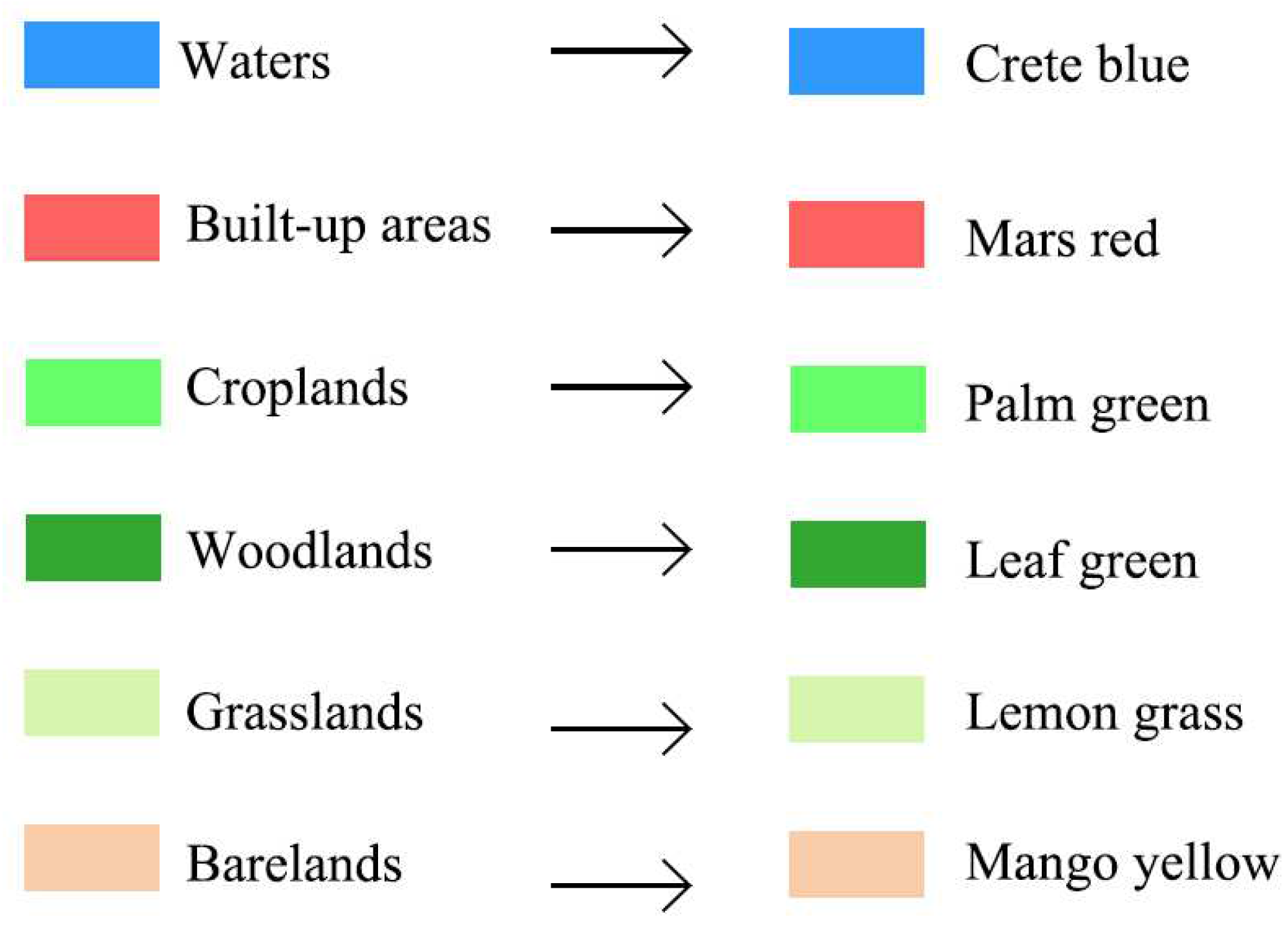
Table 2. Main land use/cover (LUC) categories.
Final Land Use TypesDescriptions
WatersRiver channels, lakes, reservoirs, ponds, and wetlands
Built-up areasUrban construction, rural settlements, industrial and mining areas, and infrastructures
CroplandsPaddy fields, other irrigated lands, and sown areas
WoodlandsIncluding local patches of forests, woodlands, and shrublands
GrasslandsNatural grasslands and pastures
Barelands Bare soil and bare rocks
Table 3. Remaining drivers, limiters, and their symbols.
Factor TypesPotential FactorsUnitsVariable Symbol
Natural factorsElevationmD1
Slope°D2
Geographic factorsDistance to roadsmD3
Distance to motorwaysmD4
Distance to railwaysmD5
Distance to lakes/reservoirsmD6
Distance to riversmD7
Distance to urban residential areasmD8
Socioeconomic factorsPopulation densityPersons/km2D9
Average GDP per unit landYuans/ km2D10
Constraining factorsProtected farmlands-L1
Protected areas of first-class water source-L2
National forest parks-L3
Main urban areas-L4
Table 4. Collinearity diagnosis of the driving factors using variance inflation factor (VIF).
Land Use TypesD1D2D3D4D5D6D7D8D9D10
Waters2.1391.7931.1631.7021.5951.2551.4371.2356.9617.304
Built-up areas1.7501.4771.1981.5441.6981.1221.3801.1315.3555.637
Croplands1.9781.7451.1571.5131.6071.1181.3381.1285.7386.061
Woodlands2.1011.9581.1902.0742.1231.3011.3151.2387.0217.607
Grasslands1.9121.5381.1811.4661.6321.1231.4591.1277.0237.256
Barelands1.7221.3751.1621.2111.2681.0931.4901.0906.6756.990
Table 5. Accuracy of LUC classification.
YearOAKCPAUA
201096.36%0.932996.36%99.18%
201598.66%0.973398.66%98.66%
202097.67%0.956697.67%97.67%
Table 6. Land use/cover (LUC) types and LUC changes from 2010 to 2020.
LUC Types201020152020LUC Changes (km2)
Area (km2)%Area (km2)%Area (km2)%2015–20102020–20152020–2010
Built-up Areas2094.7518.352394.8620.982899.4425.40300.11504.58804.69
Waters1240.1310.861296.4611.361110.419.7356.33−186.05−129.72
Croplands7037.4161.656734.7558.996469.2756.67−302.66−265.48−568.14
Woodlands713.566.25695.126.09681.545.97−18.44−13.58−32.02
Grasslands66.620.5860.900.5349.650.43−5.72−11.25−16.97
Barelands263.712.31234.092.05205.871.80−29.62−28.22−57.84
Total11,416.18100.0011,416.18100.0011,416.18100.000.000.000.00
Table 7. Accuracy comparison of different models.
Kappa ValuesCMLCMMCMLMCM
Kno0.77860.76160.79840.8156
Kstandard0.71660.69490.73980.7612
Klocation0.73130.70920.77470.8025
Table 8. Predicted land use/cover (LUC) pattern in 2025.
TypesWatersBuilt-Up AreasCroplandsWoodlandsGrasslandsBarelands
Area (km2)950.743342.836175.13643.8559.77243.85
Δ2025–2020 (km2)−159.67443.39−294.14−37.6910.1237.98
Annual average change (km2)−31.9388.68−58.837.542.027.60
Table 9. Comparison of the model features.
Hybrid ModelDriving FactorsConstraining
Factors
Expert Knowledge IntegrationAnalysis of Drivers and Constraining Factors
Markov ModelNoNoNoNo
CMNoNoNoNo
LCMYesNoNoLR
MCMYesYesYesMCE
LMCMYesYesNoLR, MCE
Disclaimer/Publisher’s Note: The statements, opinions and data contained in all publications are solely those of the individual author(s) and contributor(s) and not of MDPI and/or the editor(s). MDPI and/or the editor(s) disclaim responsibility for any injury to people or property resulting from any ideas, methods, instructions or products referred to in the content.

