Identification of Ecological Risk “Source-Sink” Landscape Functions of Resource-Based Region: A Case Study in Liaoning Province, China

Abstract

Ecological risk assessment plays an important role in ecosystem management and conservation. Conventional landscape-level assessment can only estimate the ecological risk level. It does not define ecological risk types, resulting in a lack of targeted regulation methods. This study establishes a model for identifying ecological risk-related “source-sink” landscape functions according to (1) “source-sink” landscape theory, (2) the responses of landscape types to ecological risks, and (3) the key influences on ecological risk. Four ecological risk “source-sink” landscape functions were mapped as a grid to understand their distribution. Natural and human activity factors were analyzed to determine their effects. After comprehensively considering the ecological risk levels, types of ecological risk, “source-sink” landscape functions, and their influencing factors, six principles and twenty-four targeted regulation strategies were proposed. Take the Liaoning province, China, as an example. The results prove that more than 80% of the grids were affected by the ecological risk “sink” landscape function for different and multiple ecological risks in the study area. Landscapes with the “source” function were mainly located in central cities and coastal areas. About 65% of the grids with “sink” landscape functions had medium, moderate-high, and high ecological risks. More than 75% of the grids with “source” landscape functions had medium, moderate-low, and low ecological risks. Local terrain features, vegetation, and climate were closely related to the “source” or “sink” landscape function of a grid. The land use type converted to artificial surface had the highest driving effects (q value) on multiple ecological risk “source-sink” landscape functions, and had a significant difference between other factors. The driving effects of land use type converted to artificial surface and road network density gradually increased with the risk level. The influences of GDP and population density gradually weakened with the level. The influence of interaction between any two factors was stronger than the influence of a single factor on ecological risk. The proposed assessment model can help to identify specific ecological risk at the grid level, and combined with the regulation strategy, the scientific basis can be provided for the regulation and management of different ecological risks.

1. Introduction

Natural ecosystems are an important material foundation and provide ecological services for the development of human society. The continuous expansion of human society has resulted in many direct and indirect ecological risks, such as soil erosion [1,2], geological disasters [3,4], urban heat islands, land desertification [5,6], water pollution, and other risks [7,8,9,10,11,12].

According to the Ministry of Emergency Management of the People’s Republic of China, the surface area subject to soil erosion in 2019 was 1.5 million km², with 5 billion tons of soil lost annually. According to the Ministry of Natural Resources of the People’s Republic of China, there were 4772 geological disasters across the country in 2021, causing direct economic losses of CNY 3.2 billion. Therefore, to better support regional ecological construction, resource management, and environmental restoration, accurate assessment of potential regional ecological risks is necessary.

Ecological risk refers to the potential adverse effects of nature or human activities on the structure and function of ecosystems [13]. An important component of ecological risk assessment, landscape ecological risk assessment, mainly focuses on administrative regions, cities, and ecologically fragile areas [14,15,16,17]. Resource-based regions and cities are expected to be research hotspots because of their ecological risk characteristics. Ecological risks in resource-based regions are mainly caused by landscape pattern changes brought about by urbanization and the physical and chemical pollution caused by irresponsible resource utilization [18]. For example, large-scale mining activities have caused landform changes, vegetation degradation, biodiversity losses, and geological disasters [19]. Urbanization has influenced agriculture [18]. The main ecological impact of mining activities on soil and water is heavy metal pollution [17]. Human activities, natural factors, and land cover types all affect local levels of ecological risk [18]. The ecological risks associated with land cover types such as ecological land around mines, agro-pastoral zones, forests, and grassland are relatively high [19]. The level of regional ecological risk can be reduced by using measures such as converting cultivated land to forest and grassland, land reclamation, and village relocation [20]. Compared with urban agglomerations that have highly developed economies, resourced-based regions have more available and potential ecological land. Due to the influences of human activities, climate changing the terrain, and other factors, some ecological land with high ecological quality is facing ecological risks, which has affected the functioning and transmission of the land’s ecological functions [20]. On the other hand, exploitation of resources has destroyed the natural environment, resulting in poor vegetation growth and a lower regional carbon sink capacity.

The study object of landscape ecological risk assessment is a collection of the regional ecosystem with high spatial heterogeneity [21]. At the landscape scale, ecological risks are caused by the interaction between the regional landscape pattern and the ecological processes present. Current research on landscape-scale ecological risk assessment mainly includes evaluation unit scale determination [15,22], modification of assessment model [18,23], and application of their results to landscape planning and management [24,25]. However, few studies have focused on the combination of ecological risks and specific ecological processes. Therefore, their ecological risk assessments do not correspond to specific ecological process, and the risk control loses its direction.

“Source-sink” landscape theory involves the study of risk sources and sinks and the mechanisms of their exposure–response processes. It facilitates understanding of the interactions between regional ecological risks and processes in the regions [19]. Currently, it has been widely used in the study of nonpoint source pollution, urban heat islands, and population dynamics [19,26,27]; however, studies on other ecological risks or processes remain relatively scarce. “Source-sink” theory originated from atmospheric science. A process that produces a gas is a “source”, while a process that consumes a gas is a “sink”. The “source-sink” landscape theory has been further enriched by research in different fields. Here, a “source” landscape is the source of ecological processes, and generally plays a facilitating role, while a “sink” landscape represents the end of ecological processes and generally shows a weakening effect. Therefore, the evaluation of “source-sink” landscape function indicates the contribution of the landscape within the evaluation unit to an ecological process. One of the keys to applying “source-sink” landscape theory to ecological risk processes is to accurately identify the corresponding “source” and “sink” landscapes [13,28].

While some regions have similar landscape structures, climatic and natural factors can also influence the final ecological risk “source-sink” landscape functions [25,29,30]. According to Huang et al., slope, elevation, and distance from a river are the main geographic influences on the “source-sink” landscape functions of nonpoint source pollution [26]. Jiang et al. considered that distance that may be affected by nonpoint source pollution is the important factor in correcting the original nonpoint pollution source-sink landscape contrast index [31]. Zhang et al. used eight factors to construct a hydrological response unit landscape contrast index (HRULCI) [32]. However, most of these studies have mainly concentrated on nonpoint pollution, and little attention has been paid to other ecological risks. Xu et al.’s study on mining areas did not correct the ecological risk results [20]. Wu et al. used NDVI, impervious surfaces, and distance to correct the results of ecological risks in mining areas; however, different types of ecological risks were not covered [19]. It is very challenging to achieve economic growth while maintaining the ecological functions of resourced-based regions. Therefore, to reflect the spatial heterogeneity of “source-sink” landscape functions of different ecological risks, the results of the ecological risk “source-sink” landscape functions need to be modified with climate and natural factors.

According to related studies [30,33,34], an ecological patch can provide multiple ecosystem functions simultaneously, meaning that it can perform multiple ecological processes. Therefore, different ecological risks may provide different “source” and “sink” landscape functions in a given region. Existing studies have not considered situations where different ecological risk “source-sink” landscape functions are integrated into ecological patches [19,20,26,31,32]. Identifying the integration of “source-sink” landscape functions of different ecological risks in the region can help to propose complete regulation strategies. The technology of integration of different ecological processes is mainly concentrated on the studies of ecological security patterns. Li et al. evaluated the multiple ecosystem functions of ecological sources by calculating four ecosystem service functions of ecological sources [30,33]. Peng et al. studied the multifunctional landscape identification in mountainous areas and the interactions between different landscape functions [34]. However, there has been little research on multiple ecological risks in resource-based regions. Therefore, it is necessary to quantify the multiple “source-sink” landscape functions related to ecological risks at the regional level.

Having a certain amount of ecological land in resource-based regions and cities helps to ensure ecosystem functioning and sustainable development [18]. Restoring the ecological environment and strengthening the carbon sink capacity of resource-based regions and cities are important measures taken by the Chinese government to achieve “carbon neutrality” [35]. This research provides a reference for areas with important ecological functions subject to environmental damage caused by mining activities. Therefore, in this study, an ecological risk assessment model based on “source-sink” landscape functions was built according to (1) “source-sink” landscape theory, (2) degree of response of landscape types to ecological risks, and (3) the factors influencing ecological risk processes. This is of great significance to the regulation and management of regional ecological risks. The research objectives of this study were: (1) to determine and modify the spatial distribution of ecological risk “source-sink” landscape functions of different types at the grid scale; (2) to determine the spatial distribution of multiple ecological risk “source-sink” landscape functions; (3) to evaluate the influence of natural and human factors on multiple ecological risk “source-sink” landscape functions; and (4) to propose a comprehensive ecological risk regulation strategy.

2. Materials and Methods

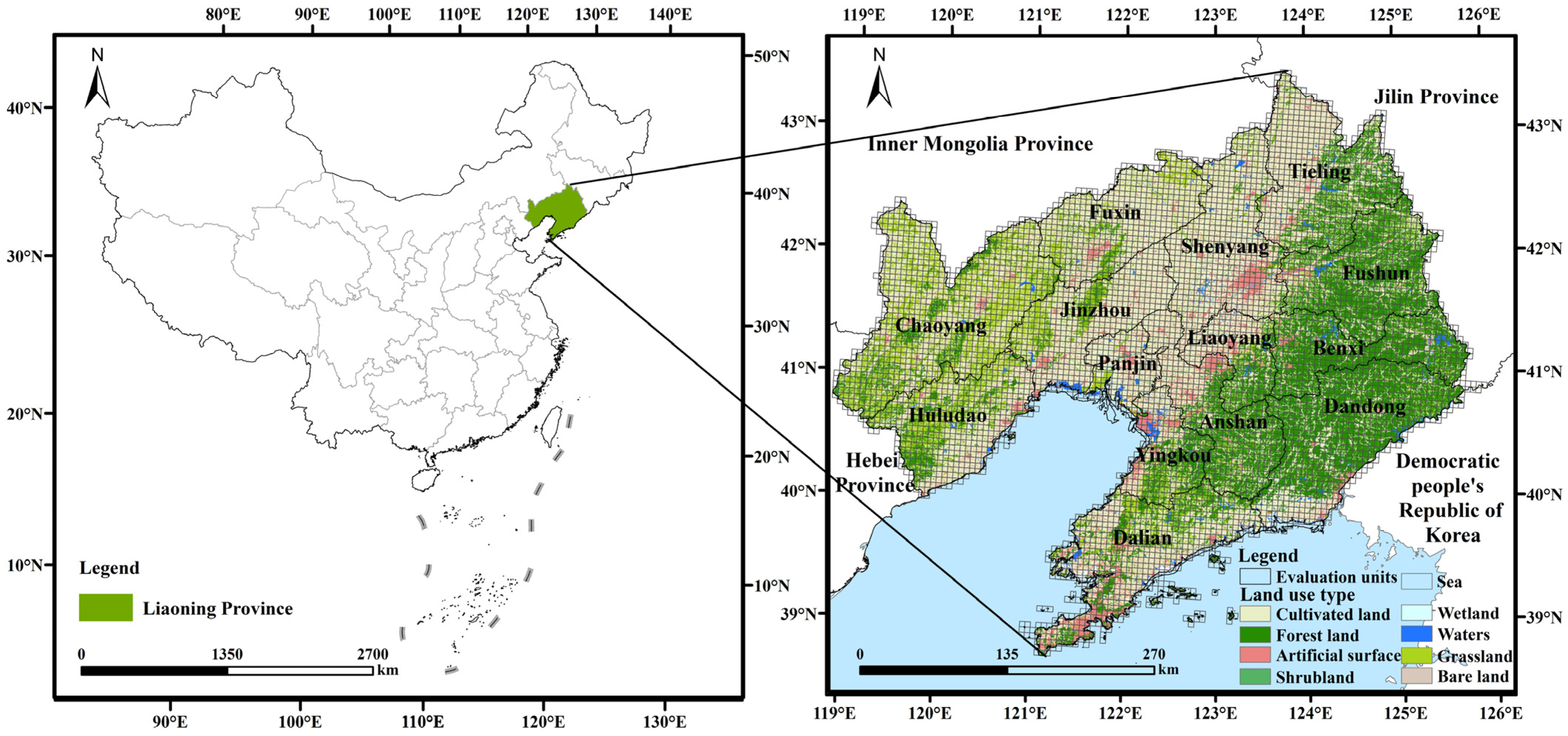
2.1. Study Area

Liaoning province (38°43′~43°26′ N, 118°53′~125°46′ E) is located in southern northeast China (Figure 1). Its total area is 148,000 km², with a mainland coastline of 2292 km, and an offshore water area of 68,000 km². It consists of 14 municipal administrative divisions. The study area has a monsoon climate typical of medium latitudes with average annual rainfall of 600–1100 mm. The average annual temperature is 7–11 °C, and the average annual sunshine is 2100–2600 h. According to the Department of Natural Resources of Liaoning Province, the ecosystems in this province includes forests, grasslands, wetlands, waterbodies, towns, cultivated land, oceans, and deserts. The forest coverage is 42%, and the total area of wetlands is 1,394,800 hectares. Liaoning Province is an important pathway for migratory birds such as the red-crowned crane and black-faced spoonbill. The development of heavy industry has brought rapid economic growth to Liaoning Province, along with severe challenges such as land degradation and environmental pollution [36]. For example, opencast mining has led to serious vegetation damage, affecting local ecological functions and surrounding natural landscapes [20]. In mining areas in high terrain with a dry climate, bare surfaces are very likely to suffer from soil erosion and soil wind erosion [37]. The hazards of underground mining cannot be ignored. Geological disasters such as land subsidence and ground fissures have destroyed a large amount of high-quality land. Ponding in mining areas wastes land resources. Meanwhile, according to China’s ecological security pattern, which is characterized by “two barriers and three belts”, Liaoning Province is located in the key areas of the Northeast Forest Belt and the North Sand Control Belt. It has important ecosystem functions, such as water conservation, biodiversity maintenance, soil conservation, and windbreak and sand fixation. It is of great significance to national and regional ecological security. At the same time, according to the national territory spatial planning of Liaoning Province, soil erosion, soil wind erosion, and mining related geological disasters are the main ecological hazards. Liaoning Province is an important grain production base, especially the black soil area, which is an extremely rare cultivated land resource. Therefore, it is necessary to restrict the conversion of cultivated land to other land use types.

2.2. Data Source

Considering the selected assessment factors affecting the risks in the study area, the data sources selected were land use type, digital elevation model (DEM), precipitation, temperature, wind speed, normalized difference vegetation index (NDVI), and mine data (

Table 1. Main data used in this study.

Data	Format	Source
Land use (2010–2020)	Grids at 30 m resolution in 2010 and 2020	GlobeLand30
SRTMDEM	Grids at 90 m resolution	Geospatial Data Cloud (China)
Precipitation (2020)	Points in 2020	China Meteorological Data Service Center (China)
Temperature (2020)
Wind speed (2020)
Normalized difference vegetation index	Grids at 250 m resolution in 2020	NASA’s 16-day L3 Global 250 m product (MOD13Q1)
Mining area	Vector	Department of Natural Resources of Liaoning Province

). Among them, land use data (30 m) of 2010 and 2020 were obtained from the GlobeLand30 website (http://www.globallandcover.com, accessed on 10 March 2021). The DEM data were provided by SRTMDEM (https://www.gscloud.cn/, accessed on 5 April 2021). The NDVI data (250 m) were obtained from MODIS (https://search.earthdata.nasa.gov/, accessed on 2 March 2021); negative values were removed and the MVC method applied to obtain yearly average data. Data on average precipitation, temperature, and wind speed were provided by the China Meteorological Data Service Center (https://data.cma.cn/, accessed on 7 May 2021). The vector data of mine data were supplied by the Department of Natural Resources of Liaoning Province. Because the original landscape data did not include mines, we superimposed the two. Using ArcGIS 10.4 software and considering relevant research and the accuracy and calculation efficiency of the results [21,38,39], the study area was divided into a 5 km × 5 km grid. A total of 6307 evaluation units (Figure 1) were obtained for subsequent calculations.

2.3. Methods

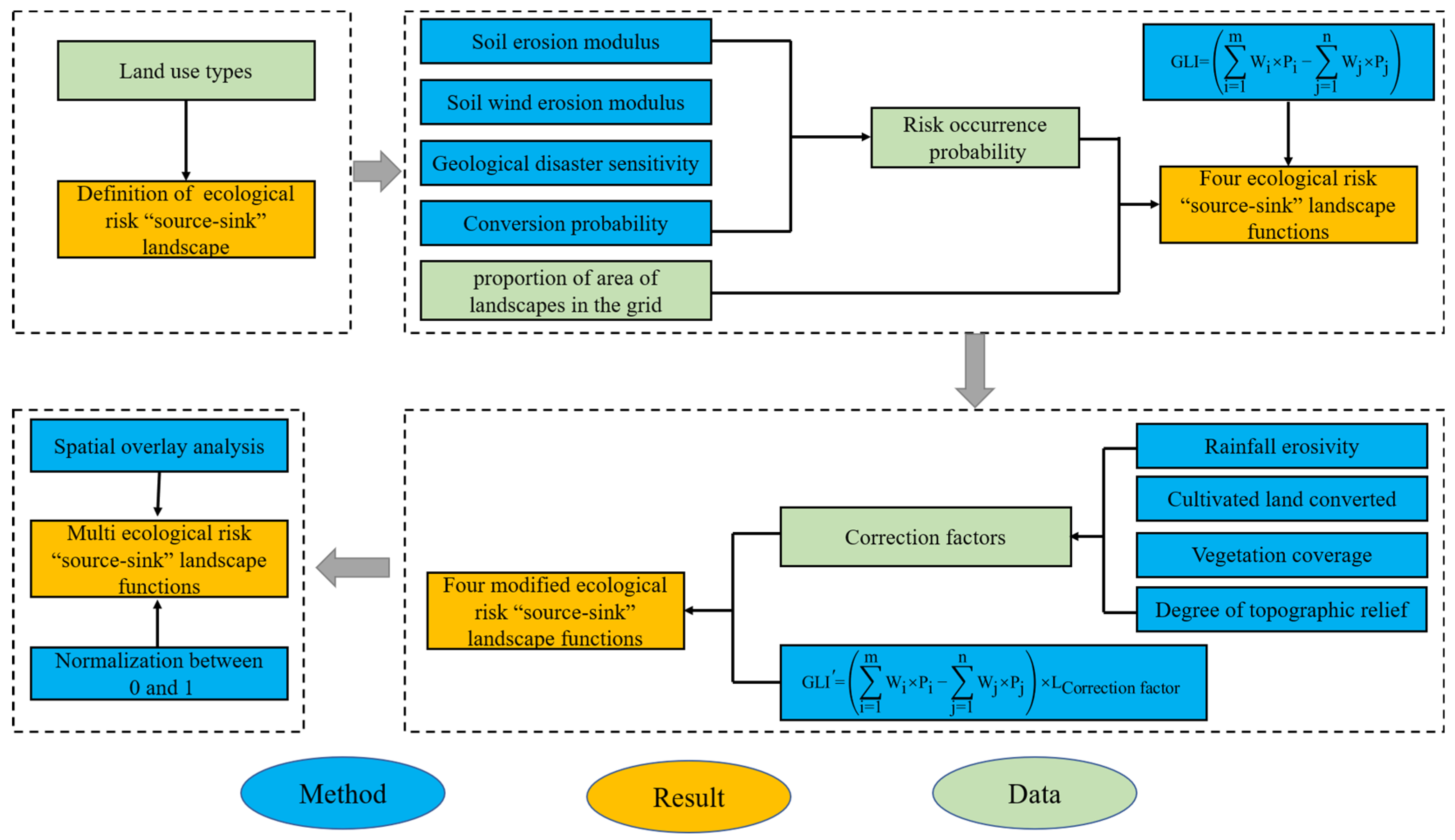
2.3.1. Classification of Ecological Risk “Source-Sink” Landscapes

In the ecological security pattern construction, the MSPA model is a widely used approach for identifying “sources”. Landscapes are divided into a foreground and background. The cores are usually identified as “sources” (the same method can also be used to identify “sink” landscapes), while other elements (such as bridges, loops, islets, edges, and branches) may also contain needed landscapes. The results of the “source” and “sink” landscapes may not be accurate, causing the identification of ecological risk “source-sink” landscape functions in some areas to be inaccurate. Therefore, based on the definition of “source” and “sink” landscapes used in the “source-sink” landscape theory used in this study, combined with the characteristics of different ecological risks, we used the approach where landscapes are directly identified as “source” or “sink” landscapes.

Referring to relevant studies, and considering the landscape types in Liaoning Province, bare land, grassland, shrubland, forest, cultivated land, water, and wetlands were considered “sink” landscapes for soil erosion [19,26]. Artificial surfaces were considered a “source” landscape for soil erosion. Cultivated land with slopes ≥ 25° are generally considered to be prone to soil erosion [40]. We calculated the slope in the study area using ArcGIS (

Table 2. Statistics of slope of cultivated land.

Landscape Type	Slope
	Min	Max	Mean	Cells of Cultivated Land of Slope ≥ 25°	Total Cells of Cultivated Land
Cultivated land	0	49.48761	3.61649	29,026	8,243,237

); the minimum value for cultivated land in Liaoning Province was 0°, the maximum value was 49.48°, and the average value was 3.61°. Cultivated land formed a total of 8,243,237 raster cells, while land with slopes ≥ 25° had 29,026 cells. Hence high slopes had little influence on the results, so cultivated land is not classified as a “source” landscape.

There are many quantitative models of soil wind erosion [41,42,43]. However, because of a lack of data on air density and soil moisture, we used previous research results. The land use types subject to soil wind erosion include forest, grassland, dry land, and sand. The land use types of non-soil wind erosion mainly include waterbodies, paddy fields, salt fields, and construction land. It is generally believed that sand has the highest soil wind erosion modulus, with those of grassland, cultivated land, and shrubland being lower, and that of forest being the smallest [44,45,46,47,48]. Vegetation coverage resists soil wind erosion; landscapes with of < 20% vegetation coverage readily suffer from soil wind erosion [49,50]. We assessed the vegetation coverage of landscapes and found that the mean values for forest, grassland, shrubland, and cultivated land in Liaoning Province were 0.82, 0.62, 0.63, and 0.45, respectively. In terms of raster cells, forest, grassland, shrubland, and cultivated land with < 20% vegetation coverage accounted for 0.04%, 0.29%, 0.18%, and 0.26%, respectively, of the total cells (

Table 3. Statistics of FVC of cultivated land, forest, grassland, and shrub land.

Landscape Type	FVC
	Min	Max	Mean	Cells of Landscapes of FVC ≤ 0.2	Total Cells of Landscapes	Percentage (%)
Cultivated land	0	1	0.45	21,563	8,243,237	0.26
Forest	0	1	0.82	2401	5,406,440	0.04
Grassland	0	1	0.62	7643	2,578,060	0.29
Shrubland	0.09343	1	0.63	4	2189	0.18

). We defined forest, grassland, shrubland, cultivated land, and bare land as “sink” landscapes. To emphasize the impact of human activities on the ecological environment, this study identified artificial surface as “source” landscapes.

Based on previous studies [19], for the risk of geological disasters of mines, bare land, grassland, shrubland, forest, cultivated land, wetland, and waters were the “sink” landscapes, and mines were the “source” landscape.

For cultivated land conversion, the landscape types converted to cultivated land are mainly forest, grassland, and artificial surfaces. However, the conversion of forest to forest and grassland may be due to local government policies such as the Sloping Land Conversion Program, and the Grain for Green policy. These policies may not increase more ecological risks in the regions [51,52]. It is assumed that the conversion of cultivated land to artificial surface causes ecological risks. Therefore, artificial surfaces were designated as a “source” landscape, while cultivated land was a “sink” landscape.

2.3.2. Calculation of Ecological Risk “Source-Sink” Landscape Functions

In the calculation of ecological risk occurrence probability in “source-sink” landscapes, the soil erosion modulus represents the difference in the degree of soil erosion between different landscape types. This study determined the risk occurrence probabilities of landscapes based on their soil erosion moduli [53,54]. According to the RUSLE model (Formula (1)), the soil erosion moduli of each landscape type were obtained, and were divided by the maximum value of the soil erosion modulus to obtain the risk occurrence probability.

A = R × K × L × S × C × P

(1)

where A is the average annual soil erosion; R is the erosivity factor of rainfall; K is the soil erodibility; L and S are the terrain factors; C is the cover management factor; and P is the support practice factor.

This study used soil wind erosion moduli to determine the ecological risk occurrence probabilities. Referring to existing research on soil wind erosion moduli in Inner Mongolia, the North China Plain, and Hebei Province, China [53,55,56,57], we obtained the soil wind erosion moduli of the landscapes. These were divided by the maximum value of the soil wind erosion moduli to determine the landscape risk occurrence probabilities.

To establish the link between landscape types and mining related geological disasters, a sensitivity coefficient was used [58,59,60]. We used the overlapping parts between mining data and original landscape data, and obtained the mine geological disaster sensitivity of landscapes according to Formula (2). The mine geological disaster sensitivity of each landscape was divided by the maximum value of mine geological disaster sensitivity to obtain the risk occurrence probabilities for the landscapes. Since only 3427 grids contain mines, the study only identifies the “source” landscapes or “sink” landscapes for these grids.

$${\mathit{SC}}_i=\left(R{\mathit{Class}}_i/\mathit{RClass}\right)$$

(2)

where SC_i is the mine geological disasters sensitivity of type i landscape; RClass_i is the area ratio of mines in type i landscape; and RClass is the area ratio of mines in all landscapes.

Referring to the idea of using land use conversion probabilities to quantify the potential degradation of ecological land [30], we used the patch-generating land use simulation (PLUS) model to obtain the conversion probabilities of cultivated land to other landscapes. Large areas of cultivated land are converted to forest and grassland due to the Grain for Green Policy of the local government, but this is not a bad thing. If these areas are treated as converted cultivated land, this may have a negative impact on the results. Therefore, this study only considered the conversion probability of cultivated land converted to the artificial surface. Since there is only one type of “source” landscape, the risk occurrence probability is 1.

Calculation of ecological risk “source-sink” landscape functions. Based on the definitions of “source-sink” landscapes, landscape risk occurrence probabilities, and the distribution of “source” and “sink” landscapes in the grid, we determined whether each grid had a “source” landscape function or “sink” landscape function (Formula (3)) [26]. For this calculation, we used 2020 landscape type data. This data included cultivated land, forest, grassland, shrubland, wetland, waters, artificial surface, and bare land landscape types. The landscape risk occurrence probabilities are calculated in before text.

$$\mathit{GLI}=\left(\sum _{I=1}^m{W}_i\times P_i-\sum _{j=1}^n{W}_j\times P_j\right)$$

(3)

where GLI is the value of a certain ecological risk “source-sink” landscape function; m is the number of “source” landscapes; i is the i-th “source” landscape; W_i is the risk occurrence probability of i-th “source” landscape; P_i is the proportion of the area of i-th “source” landscape in the grid; n is the number of “sink” landscapes; j is the j-th “sink” landscape; W_j is the risk occurrence probability of j-th “sink” landscape; and P_j is the proportion of the area of j-th “sink” landscape in the grid.

The “nature break” method was used for grading [23,61]. According to this calculation, when GLI < 0, the grid mainly has a “sink” landscape function, and when GLI > 0, this indicates a “source” landscape function.

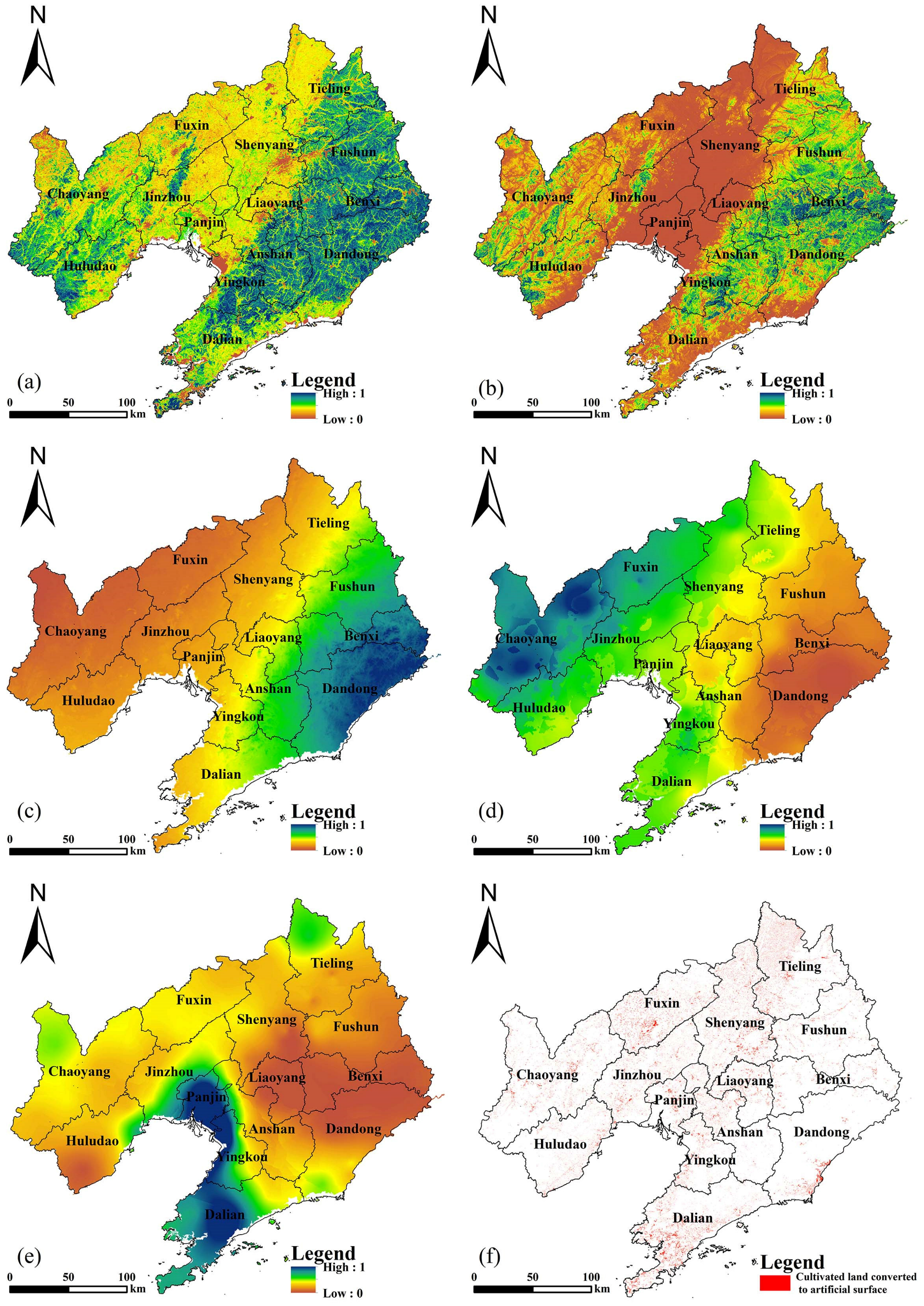
2.3.3. Calculation of Modified Ecological Risk “Source-Sink” Landscape Functions

Calculation of correction factors. To correct the ecological risk “source-sink” landscape functions, it is necessary to quantify the correction factors affecting the final contribution of ecological risks. It is also necessary to normalize the indicators involved in the correction factor, but the effects of indicators on ecological risks are different, so different normalized methods were needed.

If the indicator is positive, the normalized formula is:

$$L=\frac{l-l_{\mathit{min}}}{l_{\mathit{max}}-l_{\mathit{min}}}$$

(4)

If the indicator is negative, the normalized formula is:

$$L=\frac{l_{\mathit{max}}-l}{l_{\mathit{max}}-l_{\mathit{min}}}$$

(5)

where L is the normalized indicator; l_max is the maximum value of the indicator; l_min is the minimum value of the indicator; and l is the indicator value for the raster cell.

The slope indicator measures the topographic feature of soil erosion. The soil loss, landslide, and debris flow increase with the slope [16,62]. The study used the degree of topographic relief produced by DEM data as a topographic indicator, which is calculated in ArcGIS 10.4.1. Vegetation plays an important role in maintaining ecosystem services and reducing ecological risks [16,63]. Using a dimidiate pixel model (Formula (6)), vegetation coverage was calculated from NDVI data. The precipitation indicator represents the climate characteristics related to soil erosion. Rainfall erosivity is the potential capacity to trigger soil erosion [64,65]. Thus, rainfall erosivity is a valid indicator of soil erosion. The Wischmeier formula (Formula (7)) was used to calculate the rainfall erosivity [66]. Vegetation coverage is a negative indicator, while rainfall erosivity and degree of topographic relief are positive indicators. The three indicators were normalized separately. Based on Formula (8), a correction factor was calculated with the POWER function of the raster calculator in GIS software. For each grid, the mean correction factor was used as the correction factor of “source-sink” landscape functions of soil erosion.

$$C=({NDVI}_i-{NDVI}_{soil})/({NDVI}_{veg}-{NDVI}_{soil})$$

(6)

where C is the vegetation coverage; NDVI_i is the NDVI value of the raster cell; NDVI_veg is the NDVI value of the fully vegetated surface; and NDVI_soil is the NDVI value of the unvegetated surface.

$$R=\sum _{i=1}^{12}1.735\times {10}^{1.5\lg (\frac{p_i^2}{p}-0.8188)}$$

(7)

where R is the rainfall erosivity; p is the annual rainfall; and p_i is the rainfall of month i.

$$L_{\mathit{Correction}\mathit{factor}}=\sqrt[3]{R\times \mathit{LS}\times C}$$

(8)

where L_{correction factor} is the correction factor; R is rainfall erosivity; LS is the degree of topographic relief; and C is the vegetation coverage.

Wind speed is one of the direct sources of soil wind erosion. More days of blowing sand result in stronger wind erosion capacity. The threshold velocities are 6.0 m/s, 6.6 m/s, and 5.1 m/s for the transportation of sandy loam, loamy sandy, and fixed aeolian soil, respectively. Days with average wind speeds > 6 m/s in winter and spring (generally considered to be December–April) are suggested to be days of blowing sand. The wind speed data were filtered by observation points with Excel to obtain the days of blowing sand for each meteorological station. The Kriging interpolation method was used to map the results of days of blowing sand. Precipitation is one of the main factors affecting soil wind erosion. We used the aridity index to characterize the degree of wetness and dryness in an area. The modified Selianinov equation was used to calculate the aridity index [67,68,69] (Formula (9)). The temperature ≥ 10° in the year is the cumulative temperature of the year, and the total precipitation of days of temperature ≥ 10° in the year is the total precipitation of the cumulative temperature period. These data were used to obtain the aridity index using Formula (9) in Excel 2016. The Kriging interpolation method was used to map the aridity index results. As vegetation coverage increases, the condition of soil wind erosion decreases [70,71]. The vegetation coverage was calculated with the dimidiate pixel model (Formula (6)). For soil wind erosion, vegetation coverage is a negative indicator, and the days of blowing sand and aridity index are positive indicators. These three indicators were normalized separately. Based on Formula (10), the correct factor was calculated with the POWER function of raster calculation in GIS software. For each grid, the mean value of the correction factor was used as the correction factor of “source-sink” landscape functions of soil wind erosion.

$$I=0.16*\frac{\mathrm{Cumulative}\mathrm{temperature}\mathrm{of}\mathrm{year}}{\mathrm{total}\mathrm{precipitation}\mathrm{of}\mathrm{cumulative}\mathrm{temperature}\mathrm{period}}$$

(9)

where I is the aridity index.

$$L_{\mathit{Correction}\mathit{factor}}=\sqrt[3]{I\times W\times C}$$

(10)

where L_{correction factor} is the correction factor; I is the aridity index; W is the days of blowing of sand; and C is the vegetation coverage.

The occurrence possibility of soil erosion, landslides, and debris flows increases with the slope of the land [72]. We used the degree of topographic relief as a topographic indicator, and vegetation coverage to represent a vegetation factor [19,20]. The quantification methods for these two indicators are detailed above and in Formula (6). For the mining related geological disaster, vegetation coverage is a negative indicator, and the degree of topographic relief is a positive indicator. The two indicators were normalized separately. Based on Formula (11), the correct factor was calculated with the POWER function of raster calculation in GIS software. For each grid, the mean value of the correction factor was used as the correction factor of “source-sink” landscape functions of mining related geological disaster.

$$L_{\mathit{Correction}\mathit{factor}}=\sqrt[2]{{\mathit{LS}}_i\times C_i}$$

(11)

where L_{correction factor} is the correction factor; LS is the degree of topographic relief; and C is the vegetation coverage.

We analyzed two periods of land use data from 2010 and 2020. The land use data were resampled to 90 m, and changes in forest were obtained by reclassification and raster calculator in GIS software. The spatial distribution of cultivated land converted to artificial surfaces was obtained. We calculated the sum of cultivated land converted into artificial surfaces in the grid as a correction factor of “source-sink” landscape functions of cultivated land converted to an artificial surface. This section does not involve normalization. The formula is as follows:

$$L_{\mathit{Correction}\mathit{factor}}={\mathit{SUM}}_{\mathit{artificial}\mathit{surface}}$$

(12)

where L_{correction factor} is the correction factor; and SUM_{artificial surface} is the sum value of cultivated land converted to artificial surface in the grid.

Calculation of modified ecological risk “source-sink” landscape functions. According to the correction factors in before text related to the final contribution of ecological risks, the results of different ecological risk “source-sink” landscape functions were modified separately [19,20]. The value of GLI_i was graded by the nature break method. The judgment rules of “source-sink” landscape functions are the same as the GLI in Section 2.3.2.

$${\mathit{GLI}}^{\prime }=\left(\sum _{i=1}^m{W}_i\times P_i-\sum _{j=1}^n{W}_j\times P_j\right)\times L_{\mathit{Correction}\mathit{factor}}$$

(13)

where GLI′ is the modified certain ecological risk “source-sink” landscape functions; the significance of W_i, P_i, W_i, P_j, m, n is detailed in Formula (3); and L_{correction factor} is the correction factor of a certain ecological risk.

2.3.4. Calculation of Multiple Ecological Risk “Source-Sink” Landscape Functions

Referencing the multiple ecological patch mapping method [30,33], we quantified the multiple “source-sink” landscape function at the grid scale. The multiple ecological risk “source-sink” landscape function was determined using the following steps: (1) Its grid values were normalized to between 0 and 1; grids with values > 0 were assigned a value of 1, meaning that grids mainly perform a “source” landscape function for this ecological risk. Grids with values < 0 were assigned a value of −1, it meaning that the grids mainly perform a “sink” landscape function of this ecological risk. (2) Taking the grid as a unit, the values were subjected to spatial superposition analysis to determine the multiple ecological risk “source-sink” landscape function of the grid. The process flowchart is shown (Figure 2).

3. Results

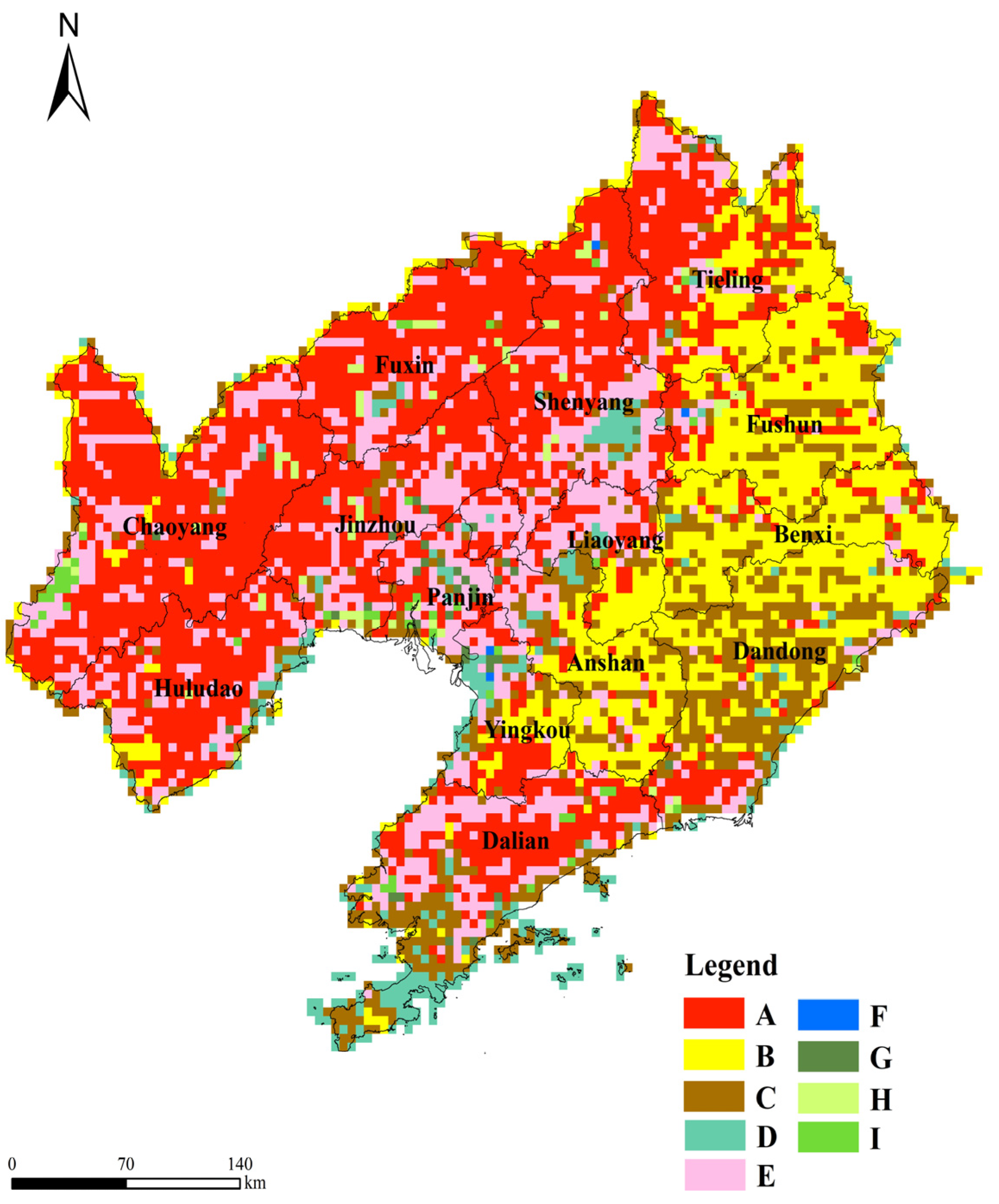
3.1. Different Ecological Risk “Source-Sink” Landscape Functions

The ecological risk occurrence probabilities for landscapes are shown in Tables S1–S4. The results of different ecological risk “source-sink” landscape functions are shown in Figure 3, and the number of grids with different ecological risk “source-sink” landscape functions is shown in Tables S5–S8. The percentage of grids performing “source-sink” landscape functions of different ecological risks at different ecological risk levels are shown in Tables S9–S12. The grids with medium, moderate-high, and high values of landscape ecological risk are most of the grids performing the ecological risk “sink” landscape function. The ecological risk levels of grids performing the “source” landscape function are mainly low and moderate-low levels. For soil erosion (Figure 3a; Table S5) and soil wind erosion (Figure 3b; Table S6), the proportion of artificial surface is relatively high in grids performing the “source” landscape function. This indicates that human activities are more frequent. In grids performing the “sink” landscape function, forest, grassland, and shrubland are widely distributed. These landscapes have high vegetation coverage and help to reduce risk. Since only cultivated land converted to artificial surface is considered, the number between grids performing the “source-sink” landscape function of cultivated land conversion was very different (Figure 3c; Table S7). The grids performing the “source” landscape function of cultivated land conversion are mainly located in the regions which have many artificial surfaces and cultivated land converted to artificial surfaces. The results and number of grids of “source-sink” landscape functions of mining related geological disasters are shown in (Figure 3d and Table S8). Grids performing the “source” landscape function of mine geological disasters have many mines, and the landscapes in the grids have high a degree of response to mine geological disasters. Most of the grids performing the “sink” landscape function have mines, but landscapes in the grids have a lesser degree of response to mine geological disasters.

3.2. Multiple Ecological Risk “Source-Sink” Landscape Functions

The result of multiple ecological risk “source-sink” landscape functions is shown in Figure 3e and

Table 4. Number and percentage of the multiple ecological risk “source-sink” landscape function.

Multiple Ecological Risk “Source-Sink” Landscape Function	Number of Grids	Percentage of Total Grids (%)
“Source” landscape function	806	12.8
“Sink” landscape function	5146	81.6
Neither of all	355	5.6

. The percentage of grids performing “source-sink” landscape function of multiple ecological risks at different ecological risk levels is shown in Table S13. According to the overlaying rule, values in the range of (1–4) represent the grids performing the multiple ecological risk “source” landscape function. A value of 4 represents a grid performing four ecological risk “source” landscape functions, and the values of 1–3 represent grids performing different ecological risk “source-sink” landscape functions, but the grid mainly performs the ecological risk “source” landscape function. Values in the range of ((−1)–(−4)) represent grids performing the multiple ecological risk “sink” landscape function. A value of (−4) represents a grid performing four ecological risk “sink” landscape functions, and the values of ((−1)–(−3)) represent grids performing different ecological risk “source-sink” landscape functions, though the grids mainly perform the ecological risk “sink” landscape functions. The value (0) is special, as it represents a grid performing two ecological risk “source” landscape functions and two ecological risk “sink” landscape functions. The number of grids performing multiple ecological risk “source-sink” landscape function is shown in Table 4. The grids with values of (1–4) are mainly located in the central and coastal areas. Grids with values of 0 are mainly distributed around grids with values of (1–4). Grids with values of ((−4)–(−3)) are mainly distributed in the east and west regions, which are related to the structure of local landscape types. Grids with values of ((−2)–(−1)) are more concentrated in the central and southern regions. These grids indicate areas that can serve to attenuate some ecological risk processes, but have the potential to induce certain ecological risk at the same time. Grids with values of (3–4) are concentrated in the central and coastal regions where nonecological landscape types dominate. The ecological risks in these regions are mainly from artificial surfaces and mines. We also found that grids with values of (1–2) and grids with a value of 0 are distributed around the grids with values of (3–4). These grids commonly perform some ecological risk “source” landscape functions, but also perform other ecological risk “sink” landscape functions.

4. Discussion

4.1. Drivers of Ecological Risk

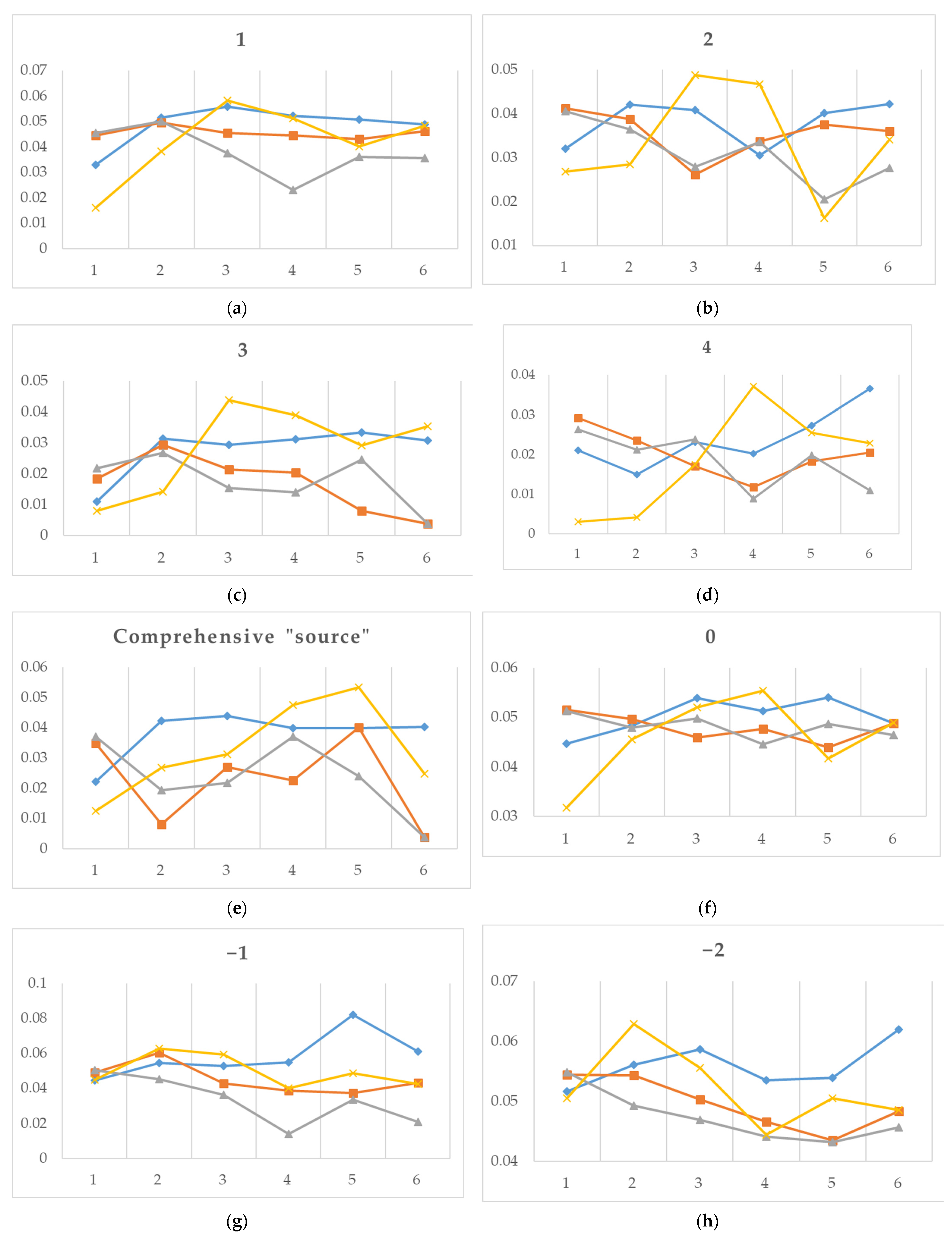
4.1.1. Analysis of the Results of Multiple Ecological Risk “Source-Sink” Landscape Functions and Ecological Risk Assessment

The higher the elevation, the greater the probability of soil erosion occurrence. Some studies show that there is no significant relationship between precipitation and erosion intensity, and splash erosion and soil detachment of runoff are affected by multiple factors [73]. The rainfall erosivity of the study area (Figure 4c) shows that the rainfall erosivity in the western regions is the lowest, but the ecological risk in the western regions is still high. The eastern and western regions have large amounts of forest and grassland, and the soil erosion modulus of these landscapes is small. Therefore, these grids mainly perform the “sink” landscape function of soil erosion.

Precipitation is one of the main factors affecting soil wind erosion. The aridity index (Figure 4d) shows that the central and western regions are relatively dry, and eastern regions are humid. As vegetation coverage increases, there will be a decrease in soil wind erosion [74]. Wind condition is also one of the driving factors causing soil wind erosion [74,75]. The more days of blowing sand in the region (Figure 4e), the higher the potential for wind erosion. The western region of the study area has a dry climate, a large amount of grassland and cultivated land, and more days of blowing sand. So, there is a possibility of soil wind erosion.

The degree of topographic relief (Figure 4b) is high in the eastern and western regions of the study area, especially in the western regions, where large amounts of grassland and cultivated land are distributed, and vegetation coverage (Figure 5a) is lower than in the eastern regions. Although the precipitation is low, there is still a high probability of soil erosion risk occurrence.

The distribution of the “source” landscape function of cultivated land conversion is generally the same as that of cultivated land converted to artificial surface (Figure 4f), and is mainly located in central and coastal regions. When there is more cultivated land converted to artificial surface, there is a higher the occurrence probability of cultivated land conversion [76,77]. Therefore, it is reasonable for grids performing the ecological risk “source” landscape function to present a high ecological risk level at the same time.

The probabilities of landslides, debris flows, and soil erosion caused by mining activities are related to the slope [72]. Vegetation cover, which plays an important role in reducing ecological risk, reflects the health of the natural ecosystem [78]. There are many mines in grids performing the “source” landscape function of mine geological disasters. The degree of topographic relief in these regions is relatively high, and mining activities have changed the land cover, which can easily lead to a series of ecological risks. The grids performing the “sink” landscape function have fewer mines, but there is also the possibility of mining related geological disasters if the topographic relief is high, and vegetation coverage is not an indicator in these grids.

4.1.2. Driving Analysis of Human Activity Factors for Ecological Risk

The density of road network, population density, GDP (GDP, and population data with 1-km grid (KMG)), and land use type converted to artificial surface were used as proxy indicators for socioeconomic development and human activity. The driving factors of ecological risk in Liaoning province (Figure 3f) were detected by the GeoDetector. The GeoDetector includes factor detector, risk detector, interaction detector, and ecological detector [77,79].

The factor detector results (Figure 5;

Table 5. The q values of factors of socioeconomic development and human activity.

	1	2	3	4	Comeprehensive “Source”	0
Density of road network	0.1692	0.0756	0.1862	0.0455	0.1452	0.0285
GDP	0.0124	0.1066	0.0446	0.0435	0.0599	0.0061
Population density	0.0165	0.0632	0.0391	0.0389	0.0656	0.0059
Land use type converted to artificial surface	0.4789	0.3307	0.3492	0.2085	0.4506	0.1384
	−1	−2	−3	−4	Comprehensive “Sink”
Density of road network	0.0851	0.0175	0.0059	0.0039	0.0086
GDP	0.0209	0.0041	0.0075	0.0043	0.00306
Population density	0.0079	0.0069	0.0001	0.0016	0.00301
Land use type converted to artificial surface	0.0976	0.0559	0.0753	0.0864	0.07874

Note: the table counts the maximum and minimum values of indicators for multiple ecological risk “source” landscape function levels. The yellow numbers represent maximum values, and red numbers represent minimum values. p values of all factors are < 0.05 and pass the significance test.

) demonstrate that land use type converted to artificial surface is the main influencing factor, and population density has the least influence on most “source-sink” landscape functions. The GDP has the least driving effect on the “source” landscape function (1 and comprehensive) and the “sink” landscape function (−2).

For the “source” landscape function and the multiple ecological risk “source-sink” landscape function of (0), the risk detector results (Figure 6) demonstrate that as the grades of the density of road network and land use type converted to artificial surface increase, the explanatory power of the influencing factors on the “source” landscape function gradually increases, and the highest values occur in the third, fourth, fifth, and sixth grades for all “source” landscape functions. The driving effects of GDP and population density fluctuate and gradually weaken. For the “source” landscape function (1, 2, 3, 4), the highest values occur in the first and second grades. The highest values occur in the fourth and fifth grades for the comprehensive “source” landscape function. For all “sink” landscape functions, the density of road network has an enhanced effect. The higher the influencing factor grade, the stronger the driving effect. The driving effect of GDP and population density gradually decreases. The driving effect of land use type converted to artificial sur-face fluctuates and gradually weakens as the grade of land use type converted to artificial surface increases.

The interactions are nonlinear enhanced and bilinear enhanced. The effect of bilinear enhanced demonstrates that the influence of interaction between any two factors is stronger than the influence of a single factor on ecological risk. The effect of nonlinear enhanced indicates that the combination of indicators can increase the influence of each single factor nonlinearly. The results (Table S14) indicate that various factors play different roles in the different “source” landscape functions.

For all “source” landscape functions, the interactions between the density of road network, GDP, and population density are nonlinear enhanced. The inter-action between the density of road network and land use type converted to artificial surface is bilinear enhanced for the “source” landscape function (1, 3, and comprehensive). The interaction between the density of road network and land use type converted to artificial surface is nonlinear enhanced for the “source” landscape function (2, 4). The interaction of GDP and land use type converted to artificial surface is nonlinear enhanced for the “source” landscape function (2, 3, 4). The interaction between these two factors is bilinear enhanced for the “source” landscape function (1, comprehensive). The interaction of GDP and population density is bilinear enhanced for the “source” landscape function (2, 4, and comprehensive), and is nonlinear enhanced for “source” landscape functions (1, 3). The interaction between population density and land use type converted to artificial surface is bilinear enhanced for the “source” landscape function (1, 4), and nonlinear enhanced for the “source” landscape function (2, 3, and comprehensive).

The interactions between two factors are nonlinear enhanced and bilinear enhanced in the different “sink” landscape functions. The density of road network and GDP show the effect of bilinear enhanced for the “sink” landscape function (−1), and show the effect of nonlinear enhanced for the others. For the “sink” landscape function (−1, −2, and −3) and “sink” landscape function (−4, -comprehensive), the interactions between the density of road network and land use type converted to artificial surface are nonlinear enhanced and bilinear enhanced. For the “sink” landscape function (−1, −3), the interaction between the GDP and land use type converted to artificial surface is bilinear enhanced. For the “sink” landscape function (−2, −4, and comprehensive), the interaction between the GDP and land use type converted to artificial surface is nonlinear enhanced. The GDP and population density are bilinear enhanced for the “sink” landscape function (−2, −3, and −4), and are nonlinear enhanced for the “sink” landscape function (−1, comprehensive). The interaction of population density and land use type converted to artificial surface is bilinear enhanced for the “sink” landscape function (−3), and nonlinear enhanced for the “sink” landscape function (−1, −2, −4, and comprehensive).

Same as the result of the multiple ecological risk “source-sink” landscape function of (2) and (−2), for the multiple ecological risk “source-sink” landscape function of (0), the interaction between the GDP and population density is bilinear enhanced, and other interactions between two factors are nonlinear enhanced.

The results of ecological detector (Table S15) show that the effect of land use type converted to artificial surface is significantly different from the effects of other factors for the multiple ecological risk “source-sink” landscape function of (0) and most “source” landscape functions. The effect of the density of road network differs from the effect of population density for the “source” landscape function (1, 3). It has a significant difference between road network density and GDP for the “source” landscape function (1, 3, and comprehensive). For all “sink” landscape functions, there is a significant difference between land use type converted to artificial surface and other factors.

4.2. Regulation Strategy Combining Ecological Risks and Ecological Risk Assessment

This study proposes comprehensive regulation strategies from the perspective of ecological risk levels, types, and “source-sink” landscape functions, as follows (Figure 7), (Table S16), (Table S17). The following principles apply to different ecological risk levels: Principles such as the restrictive development of “sink” landscapes or protection of “sink” landscapes are implemented in areas with high risk levels [16]. Principles of protective development of “sink” landscapes are carried out in areas with moderate risk levels [80,81]. In grids with low risk levels, these grids are suitable for development, and equal priority should be given to development and ecological protection [30,82].

The following regulation strategy principles apply to different ecological risk levels or “source-sink” landscape functions. Ecosystem restoration should be performed in the areas performing “source” landscape functions for the reduction of pollution and destruction [30,30]. Strategies for maintaining “sink” landscape functions should be implemented in grids performing the “sink” landscape function [25].

In grids performing “source” landscape functions and with high risk levels, high pollution-load landscapes can be converted into low pollution-load landscapes for risk reduction [26]. Therefore, the regulation strategies are mainly based on a “conversion of landscape type” focusing on abandoned mines, low-quality cultivated land, and construction land with slopes < 25 degrees. In the grids performing “source” landscape functions and of moderate-high or medium risk levels, several small “sink” landscapes (such as forests and grassland) can be supplemented to improve the ecological environment and reduce the ecological risk of human activities, without changing the “source” landscape function. Therefore, the regulation strategies are mainly based on “inlay sink landscapes”, focusing on areas with vegetation coverage < 20% and low-quality cultivated land. In grids performing the “source” landscape function and of moderate-low or low risk levels, the few high-quality ecological landscapes in the area must be protected. More attention should be paid to the ecological conservation redline, urban growth boundary, and circumventing construction in potential geological disaster areas [82]. Therefore, the regulation strategies are mainly based on the “delineation of protection areas”, focusing on landscapes with high ecological value.

In the grids performing the “sink” landscape function and of a high risk level, due to the high occurrence possibility of ecological risks, it is necessary to limit the conversion of ecological landscapes with a low pollution load to landscapes with a high pollution load to maintain the “sink” landscape function of the area. Therefore, the regulation strategies are mainly based on “restrictive conversion of landscape type”, focusing on the ecological landscape and cultivated land in the region. In grids performing the “sink” landscape function and of moderate-high to medium risk levels, the occurrence probability of ecological risks is moderate, and economic activities can be carried out under the premise of implementing a series of ecological protection measures. Therefore, the regulation strategies are mainly based on “setting a vegetative filter or forest belt around the “source” landscape” and focusing on “sink” landscapes without ecological buffer zones. In grids performing the “sink” landscape function and of moderate-low to low risk levels, the occurrence probability of ecological risks is low, so construction activities can be carried out. It is necessary to protect a large number of high-quality ecological landscapes in the area to ensure the “sink” landscape function. Therefore, the regulation strategies are mainly based on the “delineation of protection areas of high quality “sink” landscapes”, and focusing on high-quality ecological landscapes and cultivated land in the area.

4.3. Limitation and Future Work

This study has some limitations: (1) Due to a lack of data, previous research was used to calculate the landscape soil wind erosion moduli. The corrections of the results of “source-sink” landscape functions of mining related geological disasters were based on climate, terrain characteristics, and vegetation coverage factors. With further data collection, these results can be optimized. (2) Due to data limitation or some assessment parameters, we have only conducted one period of analysis, so some indicators were only calculated for a single period. With further data collection, more periods can be included, and data such as multiyear averages can be used to improve the results. More information can be gained from the perspective of a time-series analysis. (3) The impacts of mining may differ according to the types of mines and mining operations. Soil and water pollution caused by mining activities are also worthy of discussion. In the future, the issue of ecological risks related to mining activities can be further studied based on these aspects.

5. Conclusions

Landscape ecological risk assessment was applied to evaluate the regional ecological risk level. However, previous studies failed to take specific ecological risk into account, so ecological risk regulation strategies are not comprehensive and targeted enough. This study used a methodological framework of identifying soil erosion, soil wind erosion, cultivated land converted to artificial surface, and mining related geological disasters. Multiple ecological risk “source-sink” landscape functions were developed based on the “source-sink” landscape theory and correction factors influencing the final contribution of ecological risks. A comprehensive regulation strategy was proposed based on the level and type of ecological risk and “source-sink” landscape functions. This study provides a theoretical and methodological reference for resource-based regions in identifying important “source-sink” areas of ecological risks, and proposing characteristic regulation strategies. The main conclusions are as follows:

(1) Grids with a high proportion of vegetation mostly perform the ecological risk “sink” landscape function. Grids with a large proportion of mines and artificial surface, and cultivated land converted to an artificial surface are more likely to perform the ecological risk “source” landscape function. The ecological risk level of grids performing the “sink” landscape function is higher than that of “source” grids. These conclusions increase our understanding of the level of ecological risk of resource-based regions. (2) The degrees of topography, precipitation, and vegetation coverage have great impacts on “source-sink” landscape functions of different ecological risk and multiple ecological risk. For areas performing multiple ecological risk “source-sink” landscape functions, there is greater ecological risk when there is a high degree of topography, low precipitation, and low vegetation coverage. Land use type converted to artificial surface and density of road network have significant influences on multiple ecological risk “source-sink” landscape functions. Therefore, the key to formulating an ecological risk regulation strategy for resource-based regions is to improve the quality of the natural ecosystem and control the impact of human activities. (3) According to the level and type of ecological risk and the “source and sink” landscape function, appropriate regulation strategies were developed. For grids performing the “source” landscape function, strategy principles mainly include “conversion of landscape type”, “inlay ecological landscape”, and “delineation of protection areas”. For grids performing the “sink” landscape function, strategy principles mainly include “restrictive conversion of landscape type”, “setting a vegetative filter or forest belt around the “source” landscape”, and “delineation of protection areas of high quality “sink” landscapes”. A comparison with previous research indicates that each grid has more regulation strategies. The proposed regulation strategy framework has more pertinence and is more diverse in content.

References

1. Rothacker, L.; Dosseto, A.; Francke, A.; Chivas, A.R.; Vigier, N.; Kotarba-Morley, A.M.; Menozzi, D. Impact of Climate Change and Human Activity on Soil Landscapes over the Past 12,300 Years. Sci. Rep. 2018, 8, 247. [Google Scholar] [CrossRef]
2. Niacsu, L.; Bucur, D.; Ionita, I.; Codru, I.-C. Soil Conservation Measures on Degraded Land in the Hilly Region of Eastern Romania: A Case Study from Puriceni-Bahnari Catchment. Water 2022, 14, 525. [Google Scholar] [CrossRef]
3. Xu, Y.; Tang, T.; Sun, G. Research on Planning Evaluation Index System of Residential Areas in Mountainous City for Geological Disaster Prevention—A Case. Disaster Adv. 2013, 6, 114–121. [Google Scholar]
4. Calo, F.; Calcaterra, D.; Iodice, A.; Parise, M.; Ramondini, M. Assessing the Activity of a Large Landslide in Southern Italy by Ground-Monitoring and SAR Interferometric Techniques. Int. J. Remote Sens. 2012, 33, 3512–3530. [Google Scholar] [CrossRef]
5. Kairis, O.; Kosmas, C.; Karavitis, C.; Ritsema, C.; Salvati, L.; Acikalin, S.; Alcala, M.; Alfama, P.; Atlhopheng, J.; Barrera, J.; et al. Evaluation and Selection of Indicators for Land Degradation and Desertification Monitoring: Types of Degradation, Causes, and Implications for Management. Environ. Manag. 2014, 54, 971–982. [Google Scholar] [CrossRef] [PubMed]
6. Wijitkosum, S. Reducing Vulnerability to Desertification by Using the Spatial Measures in a Degraded Area in Thailand. Land 2020, 9, 49. [Google Scholar] [CrossRef]
7. Carlsen, T.M.; Coty, J.D.; Kercher, J.R. The Spatial Extent of Contaminants and the Landscape Scale: An Analysis of the Wildlife, Conservation Biology, and Population Modeling Literature. Environ. Toxicol. Chem. Int. J. 2004, 23, 798–811. [Google Scholar] [CrossRef] [PubMed]
8. Chen, S.; Zhang, Q.; Andrews-Speed, P.; Mclellan, B. Quantitative Assessment of the Environmental Risks of Geothermal Energy: A Review. J. Environ. Manag. 2020, 276, 111287. [Google Scholar] [CrossRef] [PubMed]
9. Hope, B.K. An Examination of Ecological Risk Assessment and Management Practices. Environ. Int. 2006, 32, 983–995. [Google Scholar] [CrossRef] [PubMed]
10. Schmolke, A.; Thorbek, P.; Chapman, P.; Grimm, V. Ecological Models and Pesticide Risk Assessment: Current Modeling Practice. Environ. Toxicol. Chem. Int. J. 2010, 29, 1006–1012. [Google Scholar] [CrossRef]
11. Tixier, G.; Lafont, M.; Grapentine, L.; Rochfort, Q.; Marsalek, J. Ecological Risk Assessment of Urban Stormwater Ponds: Literature Review and Proposal of a New Conceptual Approach Providing Ecological Quality Goals and the Associated Bioassessment Tools. Ecol. Indic. 2011, 11, 1497–1506. [Google Scholar] [CrossRef]
12. Tullos, D.; Byron, E.; Galloway, G.; Obeysekera, J.; Prakash, O.; Sun, Y.-H. Review of Challenges of and Practices for Sustainable Management of Mountain Flood Hazards. Nat. Hazards 2016, 83, 1763–1797. [Google Scholar] [CrossRef]
13. Landis, W.G. Twenty Years before and Hence; Ecological Risk Assessment at Multiple Scales with Multiple Stressors and Multiple Endpoints. Hum. Ecol. Risk Assess. Int. J. 2003, 9, 1317–1326. [Google Scholar] [CrossRef]
14. Kayumba, P.M.; Chen, Y.; Mind’je, R.; Mindje, M.; Li, X.; Maniraho, A.P.; Umugwaneza, A.; Uwamahoro, S. Geospatial Land Surface-Based Thermal Scenarios for Wetland Ecological Risk Assessment and Its Landscape Dynamics Simulation in Bayanbulak Wetland, Northwestern China. Landsc. Ecol. 2021, 36, 1699–1723. [Google Scholar] [CrossRef]
15. Liu, Y.; Liu, Y.; Li, J.; Lu, W.; Wei, X.; Sun, C. Evolution of Landscape Ecological Risk at the Optimal Scale: A Case Study of the Open Coastal Wetlands in Jiangsu, China. Int. J. Environ. Res. Public Health 2018, 15, 1691. [Google Scholar] [CrossRef]
16. Luo, F.; Liu, Y.; Peng, J.; Wu, J. Assessing Urban Landscape Ecological Risk through an Adaptive Cycle Framework. Landsc. Urban Plan. 2018, 180, 125–134. [Google Scholar] [CrossRef]
17. Peng, J.; Zong, M.; Hu, Y.; Liu, Y.; Wu, J. Assessing Landscape Ecological Risk in a Mining City: A Case Study in Liaoyuan City, China. Sustainability 2015, 7, 8312–8334. [Google Scholar] [CrossRef]
18. Liu, S.; Wang, D.; Lei, G.; Li, H.; Li, W. Elevated Risk of Ecological Land and Underlying Factors Associated with Rapid Urbanization and Overprotected Agriculture in Northeast China. Sustainability 2019, 11, 6203. [Google Scholar] [CrossRef]
19. Wu, J.; Zhu, Q.; Qiao, N.; Wang, Z.; Sha, W.; Luo, K.; Wang, H.; Feng, Z. Ecological Risk Assessment of Coal Mine Area Based on “Source-Sink” Landscape Theory—A Case Study of Pingshuo Mining Area. J. Clean. Prod. 2021, 295, 126371. [Google Scholar] [CrossRef]
20. Xu, W.; Wang, J.; Zhang, M.; Li, S. Construction of Landscape Ecological Network Based on Landscape Ecological Risk Assessment in a Large-Scale Opencast Coal Mine Area. J. Clean. Prod. 2021, 286, 125523. [Google Scholar] [CrossRef]
21. Lin, Y.; Hu, X.; Zheng, X.; Hou, X.; Zhang, Z.; Zhou, X.; Qiu, R.; Lin, J. Spatial Variations in the Relationships between Road Network and Landscape Ecological Risks in the Highest Forest Coverage Region of China. Ecol. Indic. 2019, 96, 392–403. [Google Scholar] [CrossRef]
22. Ju, H.; Niu, C.; Zhang, S.; Jiang, W.; Zhang, Z.; Zhang, X.; Yang, Z.; Cui, Y. Spatiotemporal Patterns and Modifiable Areal Unit Problems of the Landscape Ecological Risk in Coastal Areas: A Case Study of the Shandong Peninsula, China. J. Clean. Prod. 2021, 310, 127522. [Google Scholar] [CrossRef]
23. Cui, L.; Zhao, Y.; Liu, J.; Han, L.; Ao, Y.; Yin, S. Landscape Ecological Risk Assessment in Qinling Mountain. Geol. J. 2018, 53, 342–351. [Google Scholar] [CrossRef]
24. Kapustka, L.A.; Bowers, K.; Isanhart, J.; Martinez-Garza, C.; Finger, S.; Stahl, R.G., Jr.; Stauber, J. Coordinating Ecological Restoration Options Analysis and Risk Assessment to Improve Environmental Outcomes. Integr. Environ. Assess. Manag. 2016, 12, 253–263. [Google Scholar] [CrossRef] [PubMed]
25. Liu, Y.; Peng, J.; Zhang, T.; Zhao, M. Assessing Landscape Eco-Risk Associated with Hilly Construction Land Exploitation in the Southwest of China: Trade-off and Adaptation. Ecol. Indic. 2016, 62, 289–297. [Google Scholar] [CrossRef]
26. Huang, N.; Lin, T.; Guan, J.; Zhang, G.; Qin, X.; Liao, J.; Liu, Q.; Huang, Y. Identification and Regulation of Critical Source Areas of Non-Point Source Pollution in Medium and Small Watersheds Based on Source-Sink Theory. Land 2021, 10, 668. [Google Scholar] [CrossRef]
27. Rudra, R.P.; Mekonnen, B.A.; Shukla, R.; Shrestha, N.K.; Goel, P.K.; Daggupati, P.; Biswas, A. Currents Status, Challenges, and Future Directions in Identifying Critical Source Areas for Non-Point Source Pollution in Canadian Conditions. Agriculture 2020, 10, 468. [Google Scholar] [CrossRef]
28. Sun, R.; Xie, W.; Chen, L. A Landscape Connectivity Model to Quantify Contributions of Heat Sources and Sinks in Urban Regions. Landsc. Urban Plan. 2018, 178, 43–50. [Google Scholar] [CrossRef]
29. Huang, D.; Zhu, S.; Liu, T. Are There Differences in the Forces Driving the Conversion of Different Non-Urban Lands into Urban Use? A Case Study of Beijing. Environ. Sci. Pollut. Res. 2022, 29, 6414–6432. [Google Scholar] [CrossRef]
30. Li, S.; Zhao, Y.; Xiao, W.; Yue, W.; Wu, T. Optimizing Ecological Security Pattern in the Coal Resource-Based City: A Case Study in Shuozhou City, China. Ecol. Indic. 2021, 130, 108026. [Google Scholar] [CrossRef]
31. Jiang, M.; Chen, H.; Chen, Q. A Method to Analyze “Source-Sink” Structure of Non-Point Source Pollution Based on Remote Sensing Technology. Environ. Pollut. 2013, 182, 135–140. [Google Scholar] [CrossRef] [PubMed]
32. Zhang, X.; Cui, J.; Liu, Y.; Wang, L. Geo-Cognitive Computing Method for Identifying “Source-Sink” Landscape Patterns of River Basin Non-Point Source Pollution. Int. J. Agric. Biol. Eng. 2017, 10, 55–68. [Google Scholar] [CrossRef]
33. Li, S.; Xiao, W.; Zhao, Y.; Lv, X. Incorporating Ecological Risk Index in the Multi-Process MCRE Model to Optimize the Ecological Security Pattern in a Semi-Arid Area with Intensive Coal Mining: A Case Study in Northern China. J. Clean. Prod. 2020, 247, 119143. [Google Scholar] [CrossRef]
34. Peng, J.; Hu, X.; Qiu, S.; Meersmans, J.; Liu, Y. Multifunctional Landscapes Identification and Associated Development Zoning in Mountainous Area. Sci. Total Environ. 2019, 660, 765–775. [Google Scholar] [CrossRef]
35. Qiu, S.; Yu, Q.; Niu, T.; Fang, M.; Guo, H.; Liu, H.; Li, S.; Zhang, J. Restoration and Renewal of Ecological Spatial Network in Mining Cities for the Purpose of Enhancing Carbon Sinks: The Case of Xuzhou, China. Ecol. Indic. 2022, 143, 109313. [Google Scholar] [CrossRef]
36. Li, W.; Wang, D.; Liu, S.; Zhu, Y. Measuring Urbanization-Occupation and Internal Conversion of Peri-Urban Cultivated Land to Determine Changes in the Peri-Urban Agriculture of the Black Soil Region. Ecol. Indic. 2019, 102, 328–337. [Google Scholar] [CrossRef]
37. Wu, Z.; Lei, S.; Lu, Q.; Bian, Z. Impacts of Large-Scale Open-Pit Coal Base on the Landscape Ecological Health of Semi-Arid Grasslands. Remote Sens. 2019, 11, 1820. [Google Scholar] [CrossRef]
38. Chen, X.; Xu, D.; Fadelelseed, S.; Li, L. Spatiotemporal Analysis and Control of Landscape Eco-Security at the Urban Fringe in Shrinking Resource Cities: A Case Study in Daqing, China. Int. J. Environ. Res. Public Health 2019, 16, 4640. [Google Scholar] [CrossRef] [PubMed]
39. Jia, Y.; Tang, X.; Liu, W. Spatial–Temporal Evolution and Correlation Analysis of Ecosystem Service Value and Landscape Ecological Risk in Wuhu City. Sustainability 2020, 12, 2803. [Google Scholar] [CrossRef]
40. Xu, Y.; Yang, B.; Liu, G.; Liu, P. Topographic Differentiation Simulation of Crop Yield and Soil and Water Loss on the Loess Plateau. J. Geogr. Sci. 2009, 19, 331–339. [Google Scholar] [CrossRef]
41. de Oro, L.A.; Colazo, J.C.; Buschiazzo, D.E. RWEQ–Wind Erosion Predictions for Variable Soil Roughness Conditions. Aeolian Res. 2016, 20, 139–146. [Google Scholar] [CrossRef]
42. Pi, H.; Sharratt, B.; Feng, G.; Lei, J. Evaluation of Two Empirical Wind Erosion Models in Arid and Semi-Arid Regions of China and the USA. Environ. Model. Softw. 2017, 91, 28–46. [Google Scholar] [CrossRef]
43. Wang, W.; Samat, A.; Ge, Y.; Ma, L.; Tuheti, A.; Zou, S.; Abuduwaili, J. Quantitative Soil Wind Erosion Potential Mapping for Central Asia Using the Google Earth Engine Platform. Remote Sens. 2020, 12, 3430. [Google Scholar] [CrossRef]
44. Li, D.; Xu, E.; Zhang, H. Bidirectional Coupling between Land-Use Change and Desertification in Arid Areas: A Study Contrasting Intracoupling and Telecoupling. Land Degrad. Dev. 2022, 33, 221–234. [Google Scholar] [CrossRef]
45. Ge, X.; Ni, J.; Li, Z.; Hu, R.; Ming, X.; Ye, Q. Quantifying the Synergistic Effect of the Precipitation and Land Use on Sandy Desertification at County Level: A Case Study in Naiman Banner, Northern China. J. Environ. Manag. 2013, 123, 34–41. [Google Scholar]
46. Ying, B.; Xiao, S.; Xiong, K.; Cheng, Q.; Luo, J. Comparative Studies of the Distribution Characteristics of Rocky Desertification and Land Use/Land Cover Classes in Typical Areas of Guizhou Province, China. Environ. Earth Sci. 2014, 71, 631–645. [Google Scholar] [CrossRef]
47. You, H. Orienting Rocky Desertification towards Sustainable Land Use: An Advanced Remote Sensing Tool to Guide the Conservation Policy. Land Use Policy 2017, 61, 171–184. [Google Scholar] [CrossRef]
48. Yu, W.; Yao, X.; Shao, L.; Liu, J.; Shen, Y.; Zhang, H. Classification of Desertification on the North Bank of Qinghai Lake. Comput. Mater. Contin. 2022, 72, 695–711. [Google Scholar] [CrossRef]
49. Wu, Z.; Wang, M.; Zhang, H.; Du, Z. Vegetation and Soil Wind Erosion Dynamics of Sandstorm Control Programs in the Agro-Pastoral Transitional Zone of Northern China. Front. Earth Sci. 2019, 13, 430–443. [Google Scholar] [CrossRef]
50. Yan, Y.; Xu, X.; Xin, X.; Yang, G.; Wang, X.; Yan, R.; Chen, B. Effect of Vegetation Coverage on Aeolian Dust Accumulation in a Semiarid Steppe of Northern China. Catena 2011, 87, 351–356. [Google Scholar] [CrossRef]
51. Bullock, A.; King, B. Evaluating China’s Slope Land Conversion Program as Sustainable Management in Tianquan and Wuqi Counties. J. Environ. Manag. 2011, 92, 1916–1922. [Google Scholar] [CrossRef]
52. Wang, J.; Liu, Y.; Liu, Z. Spatio-Temporal Patterns of Cropland Conversion in Response to the “Grain for Green Project” in China’s Loess Hilly Region of Yanchuan County. Remote Sens. 2013, 5, 5642–5661. [Google Scholar] [CrossRef]
53. Du, H.; Dou, S.; Deng, X.; Xue, X.; Wang, T. Assessment of Wind and Water Erosion Risk in the Watershed of the Ningxia-Inner Mongolia Reach of the Yellow River, China. Ecol. Indic. 2016, 67, 117–131. [Google Scholar] [CrossRef]
54. Zhang, Z.; Luo, J.; Chen, B. Spatially Explicit Quantification of Total Soil Erosion by RTK GPS in Wind and Water Eroded Croplands. Sci. Total Environ. 2020, 702, 134716. [Google Scholar] [CrossRef]
55. Li, J.; Ma, X.; Zhang, C. Predicting the Spatiotemporal Variation in Soil Wind Erosion across Central Asia in Response to Climate Change in the 21st Century. Sci. Total Environ. 2020, 709, 136060. [Google Scholar] [CrossRef]
56. Liang, H.; Yian, M.; Qian, J.; Zhang, H.; Song, J. Soil Wind Erosion Characteristics and Influence Factors in Ningxia Based on Wind Erosion Model. Res. Soil Water Conserv. 2019, 26, 34–40. [Google Scholar]
57. Chi, W.F.; Kuang, W.H.; Jia, J.; Liu, Z.J. Study on Dynamic Remote Sensing Monitoring of LUCC and Soilwind Erosion Intensity in the Beijing-Tianjin Sandstorm Source Control Project Region. Remote Sens. Technol. Appl. 2019, 33, 965–974. [Google Scholar]
58. Ikemi, H. Geologically Constrained Changes to Landforms Caused by Human Activities in the 20th Century: A Case Study from Fukuoka Prefecture, Japan. Appl. Geogr. 2017, 87, 115–126. [Google Scholar] [CrossRef]
59. Lin, J.; Lin, M.; Chen, W.; Zhang, A.; Qi, X.; Hou, H. Ecological Risks of Geological Disasters and the Patterns of the Urban Agglomeration in the Fujian Delta Region. Ecol. Indic. 2021, 125, 107475. [Google Scholar] [CrossRef]
60. Zhao, Y.; Xu, X.; He, T.; Li, Y.; Hu, J. Changes of Land Use and Environment in Underground Coal Mining Area in China. Disaster Adv. 2013, 6, 125–131. [Google Scholar]
61. Mo, W.; Wang, Y.; Zhang, Y.; Zhuang, D. Impacts of Road Network Expansion on Landscape Ecological Risk in a Megacity, China: A Case Study of Beijing. Sci. Total Environ. 2017, 574, 1000–1011. [Google Scholar] [CrossRef] [PubMed]
62. Donjadee, S.; Tingsanchali, T. Reduction of Runoff and Soil Loss over Steep Slopes by Using Vetiver Hedgerow Systems. Paddy Water Environ. 2013, 11, 573–581. [Google Scholar] [CrossRef]
63. Jiang, Z.; Huete, A.R.; Didan, K.; Miura, T. Development of a Two-Band Enhanced Vegetation Index without a Blue Band. Remote Sens. Environ. 2008, 112, 3833–3845. [Google Scholar] [CrossRef]
64. Wang, X.-D.; Zhong, X.-H.; Fan, J.-R. Spatial Distribution of Soil Erosion Sensitivity on the Tibet Plateau. Pedosphere 2005, 15, 465–472. [Google Scholar]
65. Zhang, R.; Liu, X.; Heathman, G.C.; Yao, X.; Hu, X.; Zhang, G. Assessment of Soil Erosion Sensitivity and Analysis of Sensitivity Factors in the Tongbai–Dabie Mountainous Area of China. Catena 2013, 101, 92–98. [Google Scholar] [CrossRef]
66. Wu, L.; Liu, X.; Ma, X. Spatiotemporal Distribution of Rainfall Erosivity in the Yanhe River Watershed of Hilly and Gully Region, Chinese Loess Plateau. Environ. Earth Sci. 2016, 75, 315. [Google Scholar] [CrossRef]
67. Meng, M.; Ni, J.; Zhang, Z.-G. Aridity Index and Its Applications in Geo-Ecological Study. Chin. J. Plant Ecol. 2004, 28, 853. [Google Scholar]
68. Wang, Y.L. The Summae Concerning Arid Meteorological Targets to Establish, Quote and Test in China. Arid Land Geogr 1990, 3, 80–86. [Google Scholar]
69. Zhang, C.H.; Wang, M.J.; Li, X.H.; Guo, R.; Zhang, L.W. The Characteristics of Temporal and Spatial Distribution of Climate Dry-Wet Conditions over Inner Mongolia in Recent 30 Years. J. Arid Land Resour. Environ. 2011, 25, 70–75. [Google Scholar]
70. Mandakh, N.; Tsogtbaatar, J.; Dash, D.; Khudulmur, S. Spatial Assessment of Soil Wind Erosion Using WEQ Approach in Mongolia. J. Geogr. Sci. 2016, 26, 473–483. [Google Scholar] [CrossRef]
71. Zhou, Y.; Guo, B.; Wang, S.; Tao, H. An Estimation Method of Soil Wind Erosion in Inner Mongolia of China Based on Geographic Information System and Remote Sensing. J. Arid Land 2015, 7, 304–317. [Google Scholar] [CrossRef]
72. Menegaki, M.E.; Kaliampakos, D.C. Evaluating Mining Landscape: A Step Forward. Ecol. Eng. 2012, 43, 26–33. [Google Scholar] [CrossRef]
73. Marzen, M.; Iserloh, T.; Casper, M.C.; Ries, J.B. Quantification of Particle Detachment by Rain Splash and Wind-Driven Rain Splash. Catena 2015, 127, 135–141. [Google Scholar] [CrossRef]
74. Zhang, F.; Wang, J.; Zou, X.; Mao, R.; Gong, D.; Feng, X. Wind Erosion Climate Change in Northern China During 1981–2016. Int. J. Disaster Risk Sci. 2020, 11, 484–496. [Google Scholar] [CrossRef]
75. Qing, H.E.; XingHua, Y.; Ali Mamtimin, S.T. Impact Factors of Soil Wind Erosion in the Center of Taklimakan Desert. J. Arid Land 2011, 3, 9–14. [Google Scholar] [CrossRef]
76. Zhan, J.; Shi, N.; He, S.; Lin, Y. Factors and Mechanism Driving the Land-Use Conversion in Jiangxi Province. J. Geogr. Sci. 2010, 20, 525–539. [Google Scholar] [CrossRef]
77. Zhou, Y.; Li, X.; Liu, Y. Land Use Change and Driving Factors in Rural China during the Period 1995-2015. Land Use Policy 2020, 99, 105048. [Google Scholar] [CrossRef]
78. Wu, Z.; Lei, S.; He, B.-J.; Bian, Z.; Wang, Y.; Lu, Q.; Peng, S.; Duo, L. Assessment of Landscape Ecological Health: A Case Study of a Mining City in a Semi-Arid Steppe. Int. J. Environ. Res. Public Health 2019, 16, 752. [Google Scholar] [CrossRef] [PubMed]
79. Guo, L.; Liu, R.; Men, C.; Wang, Q.; Miao, Y.; Shoaib, M.; Wang, Y.; Jiao, L.; Zhang, Y. Multiscale Spatiotemporal Characteristics of Landscape Patterns, Hotspots, and Influencing Factors for Soil Erosion. Sci. Total Environ. 2021, 779, 146474. [Google Scholar] [CrossRef] [PubMed]
80. Opdam, P.; Steingröver, E.; Van Rooij, S. Ecological Networks: A Spatial Concept for Multi-Actor Planning of Sustainable Landscapes. Landsc. Urban Plan. 2006, 75, 322–332. [Google Scholar] [CrossRef]
81. Sandström, U.G.; Angelstam, P.; Khakee, A. Urban Comprehensive Planning–Identifying Barriers for the Maintenance of Functional Habitat Networks. Landsc. Urban Plan. 2006, 75, 43–57. [Google Scholar] [CrossRef]
82. Cao, Q.; Zhang, X.; Lei, D.; Guo, L.; Sun, X.; Wu, J. Multi-Scenario Simulation of Landscape Ecological Risk Probability to Facilitate Different Decision-Making Preferences. J. Clean. Prod. 2019, 227, 325–335. [Google Scholar] [CrossRef]
Figure 1. Location of the study area.
Land 12 01921 g001
Figure 2. Process flowchart used in this study.
Land 12 01921 g002
Figure 3. (a) “Source-sink” landscape functions of soil erosion. (b) “Source-sink” landscape functions of soil wind erosion. (c) “Source-sink” landscape functions of cultivated land converted to artificial surface. (d) “Source-sink” landscape functions of mine geological disasters. (e) Multiple ecological risk “source-sink” landscape functions. (f) Ecological risk assessment based on landscape pattern indices. Note: in the (a,c,d) legend, ((1)–(2)) represent the high and moderate-high values of the “source” landscape function of ecological risks, and ((3)–(5)) represent the medium, moderate-high, and high values of the “sink” landscape function of ecological risks. In the (b) legend, ((1)–(3)) represent the high, moderate-high, and medium values of the “source” landscape function of ecological risk, and ((4)–(5)) represent the moderate-high, and high values of the “sink” landscape function of ecological risk. The black legend in (c,d) represents the “conversion of cultivated land to artificial surface” and “mines”. In the (e) legend, (1–4) represent the grids performing the multiple “source” landscape function of ecological risks, and ((−1)–(−4)) represent the grids performing the multiple “sink” landscape functions of ecological risks. (0) represents grids neither performing “source” landscape functions nor “sink” landscape functions.
Land 12 01921 g003
Figure 4. (a) Vegetation coverage. (b) Degree of topographic relief. (c) Rainfall erosivity. (d) Aridity index. (e) Number of days of wind and sand. (f) Cultivated land converted to artificial surface. Note: the red legend in (f) represents “cultivated land converted to artificial surface”.
Land 12 01921 g004
Figure 5. Driving forces of factors of socioeconomic development and human activity. Note: (a) represents the multiple “source” landscape function, (b) represents the multiple “sink” landscape function.
Land 12 01921 g005
Figure 6. Results of risk detection of different ecological risk levels. Note: levels 1–6 represent the grading levels of different factors. (e,k) represent the comprehensive results of all “source” or all “sink” of Multiple Ecological Risk “Source-Sink” Landscape Functions. Meanings of (ad,f,gj) can be found in the note of Figure 3e. (1)–(4) represent the “source” landscape function, (−1)–(−4) represent the “sink” landscape function, (e) represents multiple “source” landscape functions, and (j) represents multiple “sink” landscape functions.
Land 12 01921 g006aLand 12 01921 g006b
Figure 7. Regulation strategies of ecological risk “source-sink” landscape functions. Note: A. Setting a vegetative filter or forest belt around the “source” landscape. B. Delineation of protection areas of high-quality “sink” landscapes. C. Delineation of protection areas of high-quality “sink” landscapes and delineation of protection areas. D. Delineation of protection areas. E. Setting a vegetative filter or forest belt around the “source” landscape and inlay sink landscapes. F. Conversion of landscape type. G. Inlay sink landscapes. H. Restrictive conversion of landscape type. I. Restrictive conversion of landscape type and conversion of landscape type.
Land 12 01921 g007