Improved Cropland Abandonment Detection with Deep Learning Vision Transformer (DL-ViT) and Multiple Vegetation Indices

Abstract

Cropland abandonment is a worldwide problem that threatens food security and has significant consequences for the sustainable growth of the economy, society, and the natural ecosystem. However, detecting and mapping abandoned lands is challenging due to their diverse characteristics, like varying vegetation cover, spectral reflectance, and spatial patterns. To overcome these challenges, we employed Gaofen-6 (GF-6) imagery in conjunction with a Vision Transformer (ViT) model, harnessing self-attention and multi-scale feature learning to significantly enhance our ability to accurately and efficiently classify land covers. In Mianchi County, China, the study reveals that approximately 385 hectares of cropland (about 2.2% of the total cropland) were abandoned between 2019 and 2023. The highest annual abandonment occurred in 2021, with 214 hectares, followed by 170 hectares in 2023. The primary reason for the abandonment was the transformation of cropland into excavation activities, barren lands, and roadside greenways. The ViT’s performance peaked when multiple vegetation indices (VIs) were integrated into the GF-6 bands, resulting in the highest achieved results (F1 score = 0.89 and OA = 0.94). Our study represents an innovative approach by integrating ViT with 8 m multiband composite GF-6 imagery for precise identification and analysis of short-term cropland abandonment patterns, marking a distinct contribution compared to previous research. Moreover, our findings have broader implications for effective land use management, resource optimization, and addressing complex challenges in the field.

1. Introduction

Cropland abandonment is a critical worldwide concern, with an unsettling yearly trend of 12 million hectares of agricultural land being left abandoned [1]. Moreover, the consequences of abandoned lands extend beyond mere neglect as they become sources of greenhouse gas emissions, intensifying climate change and posing a threat to global food security [2,3], while some abandoned croplands may naturally transform into restored habitats, contributing to carbon sequestration [4]. The difficult terrain, marked by steep slopes, unsuitable soil settings, harsh weather, and significant distances from settlements, poses obstacles to using machinery and limits the implementation of market-driven agricultural methods. These detrimental effects underscore the urgency of comprehending the dynamics and implications of cropland abandonment, including its impact on soil erosion, deforestation, and biodiversity loss.

Cropland abandonment is a complex phenomenon [5] that has sparked considerable debate and generated a range of hypotheses within the research community. One contentious hypothesis suggests that changes in macroeconomic conditions primarily drive cropland abandonment [5]. According to this perspective, fluctuations in market prices, trade policies, and subsidies impact farmers’ profitability, leading them to abandon their cultivated land [6]. Conversely, an alternative hypothesis argues that demographic shifts and rural–urban migration [7] exert a greater influence on the process of cropland abandonment. This viewpoint suggests that, as rural populations decline and young individuals migrate to urban areas in search of better economic prospects, a scarcity of agricultural labor emerges, prompting land abandonment. Understanding the extent of abandoned croplands is essential to grasping the magnitude of the problem and its implications for greenhouse gas emissions. This knowledge empowers policymakers to develop targeted strategies and policies to mitigate environmental impacts [8]. Additionally, monitoring abandoned lands aids in identifying regions susceptible to soil erosion and deforestation as these areas often exhibit challenging topography and poor soil conditions, making them prone to degradation [9]. Implementing soil conservation and afforestation measures in such areas helps prevent further environmental degradation while promoting ecosystem resilience. Furthermore, the monitoring of abandoned lands is vital in assessing their impact on biodiversity, allowing conservationists to design targeted strategies for habitat protection and restoration [9]. The insights gleaned from monitoring abandoned lands are instrumental in executing efficient land management strategies and formulating measures to tackle the intricacies associated with cropland abandonment [8,9,10,11]. This proactive approach fosters a more sustainable and resilient agricultural landscape, mitigating the adverse effects of cropland abandonment on the planet’s health and biodiversity.

Various remote sensing methods have been used globally to detect abandoned croplands [12]. Hang et al. [13] utilized change detection and sliding window methodologies to assess the cropland abandonment and its impact on food production. However, their study relied on unauthorized land cover data spanning over 30 years, introducing potential inaccuracies. The use of low-resolution datasets like Landsat-8 and shuttle radar topography mission (SRTM) might limit the precision of their findings. Makki et al. [14] focused on soil redistribution rates, neglecting broader cropland abandonment patterns. Zhang et al. [15] used Landsat data to detect nationwide cropland abandonment, while Liu et al. [16] employed Sentinel-2 time series data. Hong et al. [17] explored spatial correlations with redundancy analysis. Still, their study may not capture the intricate dynamics of abandoned cropland. Lotfi et al. [18] investigated water-deficient agricultural landscapes using spatial metrics and Landsat images, identifying abandoned croplands based on consecutive fallow years. Luo et al. [19] used an object-based classification approach with a focus on random forest (RF) and a recurrent neural network (RNN) trained on Sentinel-2 imagery with a derived bare soil spectral index to detect abandoned lands from 2018 to 2021 [20].

Conversely, in addition to remote sensing data, certain studies [18,21,22,23,24] have also utilized individual vegetation indices (VIs), such as the normalized difference vegetation index (NDVI), to map the abandoned lands. Praticò et al. [25] conducted a comprehensive investigation employing a range of machine learning algorithms, including support vector machine (SVM), RF, and CART, in conjunction with multiple VIs for the purpose of classifying Mediterranean forest habitats. Their study focused on a mountainous natural national parks and encompassed various sites hosting ecologically significant protected forest habitats. Pastick et al. [26] employed Landsat-8 and Sentinel-2 collaboratively to delineate seasonal vegetation index (VI) patterns within a dryland setting. Considering the limitations of the aforementioned studies, it becomes evident that there are certain shortcomings in capturing the full complexity and accurate discrimination of cropland abandonment. These limitations include reliance on unauthorized or limited-duration land cover data. Moreover, these studies have mainly concentrated on employing a single or no vegetation index and disregarded the utilization of multiple VIs for the detection of cropland abandonment. Furthermore, the spatial resolution of the images employed in these studies has frequently been constrained. This is because they have relied on publicly available data with low spatial resolution, which may inadequately capture fine-scale land cover alterations or precisely detect abandoned lands.

Therefore, the proposed approach addresses these limitations by utilizing the ViT model, leading to enhancing the accuracy in the discrimination of abandoned croplands. Harnessing the ViT consistently outperformed alternative classification methods in terms of both accuracy and robustness across various land cover scenarios, showcasing its promise as a superior technique for satellite image classification. The multiple VIs approach captures a comprehensive range of vegetation characteristics, cropland abandonment patterns, and their interactions with other land cover types. Furthermore, using GF-6 imagery brings about notable improvements in classifying fine-scale land cover changes. It provides more precise information on abandoned lands compared to relying solely on publicly available data with lower spatial resolution. Our study also utilized GDP, land prices, land supply, and their growth rates to understand regional and economic dynamics. Considering all the approaches adopted in this research, our study stands apart from previous research, making a significant contribution to cropland abandonment detection. The research objectives for this study were (1) to develop a methodology integrating deep learning architecture (ViT) and VIs for precise discrimination of abandoned croplands; (2) to assess the effectiveness of the classifier in identifying abandoned areas; (3) to characterize the spatial and temporal patterns of abandoned areas; and (4) to analyze the underlying factors associated with cropland abandonment.

2. Materials and Methods

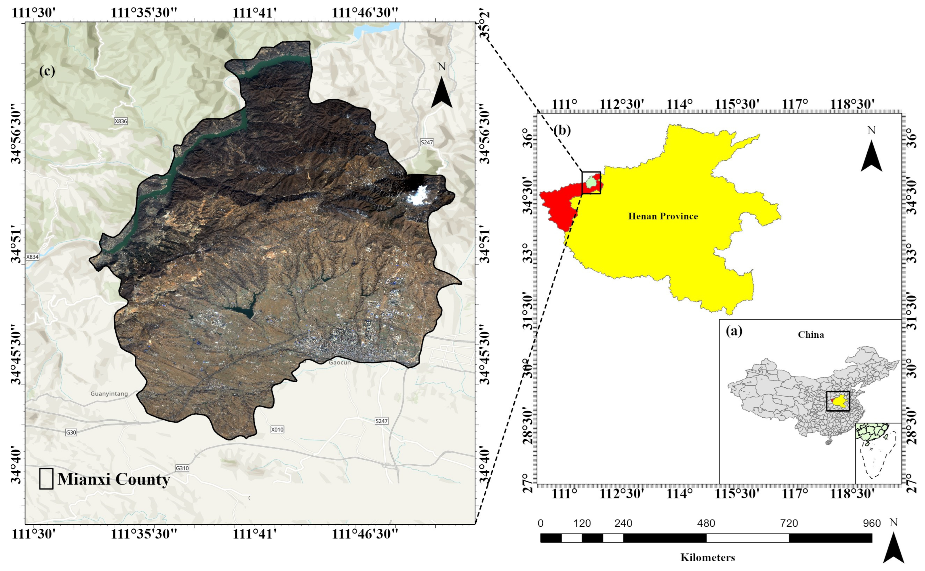
2.1. Study Area

The geographic scope of this research encompasses Mianchi County, located within Sanmenxia City in the northwestern region of Henan Province, China (Figure 1). Mianchi County is in an inland region characterized by a warm temperate monsoon climate. In winter, the area experiences a dry and cold climate with minimal rainfall and snow, largely influenced by the Mongolian cold high-pressure system. As spring approaches, the Pacific subtropical high moves northward, resulting in higher temperatures and increased precipitation. This season brings three types of weather: hot and humid, hot and dry, and rainy. In autumn, the decrease in solar altitude angle and the southward retreat of the Pacific subtropical high result in cooler climate conditions and reduced rainfall. According to the 1 November 2020 census data, Mianchi County has a population of approximately 310,130 individuals. Moreover, there has been a noticeable increase in GDP, public budget revenue, added value of industries, fixed asset investment, and retail sales of consumer goods in Mianchi since 2019 [27].

2.2. Datasets

This study utilizes the dataset from GF-6 and GF-2, Chinese civilian remote sensing satellites belonging to the “gaofen” series. Launched successfully on June 2, 2018, the GF-6 is equipped with a panchromatic multispectral camera (PMC) and wide field view camera (WFV), primarily used for precise observation of agriculture, forestry resource surveying, and related industries [28]. In certain cases, the GF-6 imagery was extensively obscured by clouds, posing a challenge to conducting any analysis. In such situations, the recourse was to use GF-2 imagery, which offers a resolution of 3.2 m.

Table 1. GF-2 and GF-6 dataset properties.

Features	GF-2		GF-6
Frequency (GHz)	8–12.5		4–8
Temporal Resolution (d)	5		1 (PMC)–4 (WFV)
Altitude (km)	631		634 km × 647 km
Swath Width (km)	One camera 23 km (45 km with two combined cameras)		95 (PMC), 860 (WFV)
Spatial Resolution (m)	PAN: 0.8	MS: 3.2	PAN: 2	MS: 8
Bands/Wavelength (μm)	Pan: 0.45–90	B1/blue: 0.45–0.52	Pan: 0.45–90	B1/blue: 0.45–0.52
		B2/green: 0.52–0.59		B2/green: 0.52–0.6
		B3/red: 0.63–0.69		B3/red: 0.63–0.69
		B4/NIR: 0.77–0.89		B4/NIR: 0.76–0.90
Cloud Coverage (%)	5–10		5–10
Date of Image Accusation (year/month/day)	2020/09/07 and 2021/10/18		2019/04/09, 2019/08/10, 2020/06/02, 2021/04/11, 2022/05/03, 2022/10/10, and 2023/04/19

comprises all the characteristics of GF-2 and GF-6. The imagery acquired from GF-6 and GF-2 includes bands such as blue (B), green (G), red (R), and near-infrared (NIR). Additionally, incorporation of a digital elevation model (DEM) with a resolution of 15 m allows for slope calculation. The DEM was acquired from the China–Brazil Earth Resources Satellite (CBERS-4), launched in 2014. CBERS-4 has a high-resolution panchromatic camera capable of capturing images with a remarkable spatial resolution of 5 m. The DEM generated from this camera provides elevation data with a resolution of 15 m. The CBERS-4 data, including the DEM, are freely accessible for download from the INPE Image Catalog (http://www.dgi.inpe.br/ accessed on 14 October 2023).

2.3. Software

Image preprocessing was conducted utilizing ENVI 5.6 software (© 2023 NV5 Geospatial, Broomfield, CA, USA). ArcGIS Pro 3.0.0 (© 2023 Esri-ArcGIS Pro, Redlands, CA, USA) was employed to calculate VIs and to create GIS mapping. For sample labeling in the classification process, Image Segmentation in eCognition Developer 9 (© 2014 Trimble-eCognition Developer 9, Westminster, CO, USA) was utilized. ArcGIS Desktop 10.6 (© 2016 Esri-ArcGIS Desktop 10.6, Redlands, CA, USA) was employed for raster conversion and change detection.

2.4. Image Preprocessing

In this study, a sequence of image preprocessing procedures was executed to augment the quality and applicability of the satellite imagery.

(1)

The first step involves the creation of subsets of the original images to focus specifically on the study area of interest, allowing for efficient computational processing and analysis of the relevant image data.

(2)

To generate multispectral imagery for our study, a layer-stacked image was assembled by combining georeferenced images. The resulting imagery consists of four bands: B, G, R, and NIR.

(3)

A color-normalized (Brovey) sharpening technique [29] was applied to convert the 8 m resolution GF-6 satellite images to 2 m resolution for sample labeling and results verification of the classifier. The Brovey Transform sharpens the multispectral image by combining it with the panchromatic image using a weighted ratio. The basic idea is to emphasize the spatial details from the panchromatic image while preserving the spectral information from the multispectral image. The technique is based on the following mathematical expression (Equation (1)):

$$S_i(x,y)=M_i(x,y)\times \frac{P(x,y)}{P_i(x,y)}$$

(1)

where $S_i(x,y)$ is the sharpened pixel value in the $i$-th spectral band at coordinates $(x,y)$. $M_i(x,y)$ is the pixel value of the multispectral image in the $i$-th spectral band at coordinates $(x,y)$. $P(x,y)$ is the pixel value of the panchromatic image at coordinates $(x,y)$. $P_i(x,y)$ is the average pixel value of the panchromatic image within the spatial neighborhood of the corresponding pixel in the multispectral image.

(4)

Since the GF-6 images sometimes did not cover the entire study area, mosaicking was conducted by merging two or more images of the same season to obtain a comprehensive view of the entire study area. This ensured that all relevant features and land cover patterns were captured in the analysis.

(5)

To ensure consistency and compatibility with other datasets, the images were projected to a standard coordinate system. This step facilitated seamless integration and comparison with other geospatial data.

(6)

Additionally, in order to derive terrain-related information, slope calculation was performed in degrees. This allowed for assessing topographic characteristics and their potential influence on land cover dynamics.

(7)

To achieve accurate reflectance values and compensate for atmospheric effects, Fast Line-of-sight Atmospheric Analysis of Spectral Hypercubes (FLAASH) atmospheric correction [30] was employed. The primary objective of FLAASH is to eliminate the atmospheric interference in remote sensing data, thereby enhancing data accuracy and reliability for a wide spectrum of applications. This correction accounted for atmospheric conditions and improved the reliability of subsequent analyses. FLAASH works according to the following mathematical formulas as in Equations (2) and (3).

$$L=\left(\frac{\mathrm{A}\rho }{1-{\rho }_{\mathrm{e}}\mathrm{S}}\right)+\left(\frac{\mathrm{B}{\rho }_{\mathrm{e}}}{1-{\rho }_{\mathrm{e}}\mathrm{S}}\right)+L_a$$

(2)

$$L_e=\left(\frac{\left(\mathrm{A}+\mathrm{B}\right){\rho }_{\mathrm{e}}}{1-{\rho }_{\mathrm{e}}\mathrm{S}}\right)+L_a$$

(3)

where $\rho$ represents the pixel’s surface reflectance, ${\rho }_{\mathrm{e}}$ denotes the average surface reflectance of the surrounding region, $S$ signifies the spherical albedo of the atmosphere, capturing the backscattered surface-reflected photons, $L$ signifies the radiance backscattered by the atmosphere without reaching the surface, and $A$ and $B$ represent surface-independent coefficients that vary with atmospheric and geometric conditions. It is important to note that all of these variables implicitly depend on wavelength.

(8)

Lastly, radiometric calibration was carried out to normalize the pixel values across the image, ensuring consistent and accurate measurements.

Figure 2 illustrates the workflow adopted in our study.

2.5. Vegetation Indices (VIs)

The use of VIs enables not only the extraction of seasonal variability within each pixel by utilizing the values of several VIs but also the utilization of these VIs as indicators [25,31,32]. Incorporating various VIs offers a complete understanding of various vegetation properties, including health, biomass, and coverage, as they dynamically evolve in response to shifting environmental conditions. Recognizing the complexity of vegetation characteristics, our study utilizes six specific VIs to ensure a well-rounded representation of diverse attributes that contribute to accurate land cover assessment (

Table 2. VIs calculated in this investigation.

VIs	Formula	Reference
Normalized Difference Vegetation Index (NDVI)	$NDVI=\frac{IR-R}{IR+R}$	[33]
Soil-Adjusted Vegetation Index (SAVI)	$SAVI=\left(\frac{NIR-R}{NIR+R+L}\right)\ast (1+L)$	[34]
Transformed Soil-Adjusted Vegetation Index (TSAVI)	$TSAVI=\frac{\left(s\right(NIR-s\ast Red-a)}{(a\ast NIR+Red-a\ast s+X\ast \left(1+s^2\right))}$	[35]
Perpendicular Vegetation Index (PVI)	$PVI=\frac{(NIR-aR-b)}{\sqrt{\left(1+a^2\right)}}$	[36]
Red-Edge Triangulated Vegetation Index (RTVICore)	$RTVIcore=\left(100\ast \left(NIR-RedEdge\right)-10\ast \left(NIR-Green\right)\right)$	[37]
Simple Ratio (SR)	$SR=\frac{NIR}{R}$	[38]

).

The normalized difference vegetation index (NDVI) stands out as the most commonly employed vegetation index due to its capability for inclusive vegetation assessment [33]. Our objective in utilizing NDVI in our research is to specifically emphasize areas with dense vegetation cover types, such as forests and cultivated lands. NDVI values range from −1 to +1.

Soil-adjusted vegetation index (SAVI) is a vegetation index that emphasizes the impact of soil brightness in areas with low vegetation coverage. Our research area is characterized by its heterogeneity, encompassing various land cover types [34]. Barren land and uncultivated areas exhibit similar brightness in imagery. To address this, the SAVI was employed to enhance the visibility of barren lands and differentiate them more effectively.

The transformed soil-adjusted vegetation index (TSAVI) is designed to decrease image brightness by assuming that the soil line has a significantly large slope and intercept [35]. In densely populated urban areas, the use of TSAVI proves valuable in distinguishing between soil and rooftop surfaces based on slope and interception, which can appear similarly bright.

The perpendicular vegetation index (PVI) incorporates an angle correction factor to address the impact of the canopy structure on reflectance measurement [36]. The utilization of PVI was chosen because approximately 30–40% of our study area is covered with forests. PVI is particularly advantageous in our case because the structure and orientation of the vegetation canopy significantly influence reflectance measurements, especially in dense forests where the observation angle affects the visibility of vegetation.

This study also utilizes the red-edge triangulated vegetation index (RTVICore) [37], a valuable tool for estimating leaf area index and biomass in vegetation. RTVICore highlights the exceptional sensitivity of the vegetation in dense biomass.

In the end, the simple ratio (SR) is employed as one of the fundamental VIs for evaluating the health and density of vegetation. This index utilizes the ratio of reflectance values in specific spectral bands and is widely utilized in remote sensing and vegetation analysis. One of the key advantages of SR is its simplicity as it does not involve any additional correction factors or transformations [38].

2.6. Optimizing Image Selection for Classifier

A well-chosen image improves classification accuracy, aids model generalization to unseen data, enhances computational efficiency, and ensures robust performance in diverse conditions. To assess the highest attainable accuracy, we swiftly tested a variety of input images for classification, distinguishing them based on different variables, including band number, reflectance regions, and VIs. We conducted F1 score and OA measurements to evaluate the influence of using one or more VIs with their potential combinations on the final classification outcome.

2.7. Classes and Image Labeling

Considering the short timeframe for detecting changes in cropland abandonment (2019–2023), the established criterion is that cropland is deemed “abandoned” if it remains inactive for agricultural purposes for two consecutive years, as stated in a study by Hou et al. [3]. The images are chosen from two distinct growing seasons: spring (April–June) and fall (September–November). Additionally, the presence of existing barren lands in our study area necessitates excluding these areas from the category of “abandoned croplands”. To ensure clarity and accuracy, six classes are defined for classification: cultivated land, uncultivated land, impervious, water, other, and forest. Cultivated land refers to land utilized for cultivating grain and cash crops during spring, fall, or both growing seasons. Uncultivated land refers to land that is either prepared for cultivation or left fallow after cultivation. The impervious class includes areas that have been urbanized or altered due to human activities in rural regions. The other class encompasses areas characterized by grassland, herbaceous, barren land, rocks, or wetlands. Lastly, the forest class includes deciduous, mixed forest, and shrubs. To identify “abandoned” pixels, we have considered those classified as “cultivated land” or “uncultivated land” in the $i$-th year but later classified as “impervious”, “water”, “other”, or “forest” in the next two years ($t+1$ and $t+2$).

The availability of GF-6-processed 2 m imagery proved highly advantageous for sample labeling in our classification process. Careful labeling was performed on approximately 700 (±50) samples for training across all years (2019–2023) for each image. The assignment included 120 labels for uncultivated land, 110 labels for cultivated land, 110 labels for impervious areas, 70 labels for water bodies, 100 labels for the other class, and 130 labels for forested areas. The generated training points were subsequently filtered, focusing on those with a minimum distance of 100 m to mitigate spatial autocorrelation [3]. The classifier was trained using 80% of the samples, with the remaining 20% reserved for testing purposes.

2.8. Cropland Abandonment Rate

For discerning spatial and temporal abandonment patterns, the rate of cropland abandonment was computed. These rates were determined by comparing the ratio of abandoned cropland to the overall cropland in the respective year. Equation (4), used to calculate the abandonment rate, is as follows:

$$C_R=\frac{A_i}{{TC}_i}\times 100\%$$

(4)

where $C_R$ denotes the ‘cropland abandonment rate’ in the $i$-th year, $A_i$ is the cropland abandoned area in $i$-th year, and ${TC}_i$ signifies the total area of cropland in $i$-th year.

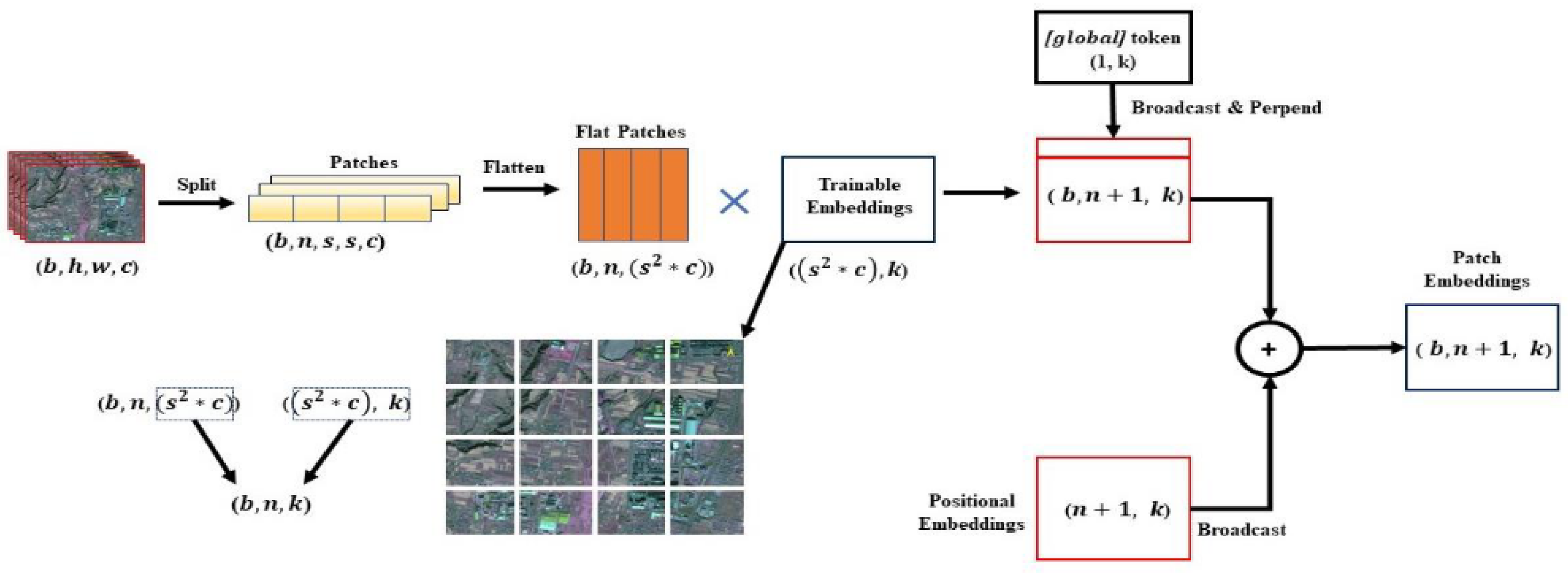
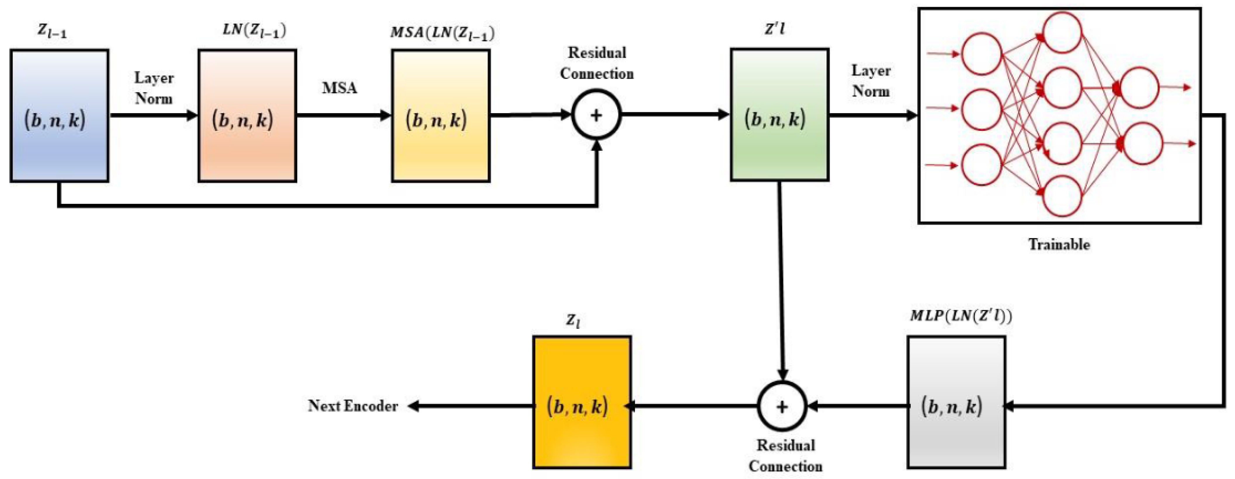
2.9. Vision Transformer Model (ViT)

Vision Transformer (ViT) was applied for image classification. ViT is a deep learning architecture designed for computer vision tasks, originally introduced by Dudovskiy et al. [39]. Unlike traditional convolutional layers, ViT employs self-attention mechanisms to capture long-range connections between different patches within an image. The input image undergoes a series of sequential transformations, ultimately yielding a feature vector of size ($n+1, k$), as illustrated in Equation (5).

$$\begin{array}{c}{z}_0=\left[x_{\mathit{class}};x_p^{1}E;x_p^{2}E,\dots ;x_p^{N}E\right]+E_{pos},\\ E\in {\mathbb{R}}^{\left(p^2.C\right)Xd},E_{pos}\in {\mathbb{R}}^{(N+1)Xd}\end{array}$$

(5)

The image is initially divided into $n$ patches, each having shapes of ($s, s, c$). These patches are then flattened into $n$ linear vectors, each with shapes of ($1, s²c$). To transform each flat patch into a new shape $k$, a trainable embedding tensor of shape ($s²c, k$) is applied, resulting in $n$ embedded patches, each with shapes of ($1, k$). Additionally, a learnable token of shape ($1, k$), denoted as [$global$], is introduced to represent an aggregate of the patch representations. The entire process of patch embedding is illustrated in Figure 3.

A stack of transformer encoders is then employed to acquire more abstract features from the embedded patches, as demonstrated in Equations (6) and (7). Layer normalization, as illustrated in Equations (8)–(11), is applied to maintain stable state dynamics, while residual connections address the challenge of vanishing gradients [40]. The learnable parameters within this component are located in the multi-head attention (MHA) mechanism and the multi-layer perceptron (MLP) weights. The MLP consists of two hidden layers with dimensions described as $w_{hidden}$ ($k,k_m{l}_p$) for the hidden layer and $w_{out}$ ($k_{m,}{l}_p, k$) for the output layer. A comprehensive overview of the transformer encoder process is presented in Figure 4.

$$z^{\prime }l=\mathrm{MSA}\left(LN\left(z_{l-1}\right)\right)+z_{l-1},l=1\dots L$$

(6)

$$z_l=\mathrm{MLP}\left(LN\left(z^{\prime }l\right)\right)+z^{\prime }l,l=1\dots L$$

(7)

$$u_i=\frac{1}{m}\sum _{j=1}^m{x}_{ij}$$

(8)

$${\sigma }_i^2=\frac{1}{m}\sum _{j=1}^m{\left(x_{ij}-u_i\right)}^2$$

(9)

$$x^{\prime }ij=\frac{x_{ij}-u_i}{\sqrt{{\sigma }_i^2+ϵ}}$$

(10)

$$y_i=\gamma x_i^{+}\beta \equiv L{N}_{\gamma ,\beta }\left(x_i\right)$$

(11)

The multi-head attention (MHA) operation, present within each of the L stacked transformers, aligns with Equations (12)–(15).

$$[q,k,v]=z{U}_{qkv},U_{qkv}\in {\mathbb{R}}^{DX3D_h}$$

(12)

$$A=\mathrm{softmax}\left(\frac{q{k}^T}{\sqrt{D_h}}\right),A\in {\mathbb{R}}^{NxN}$$

(13)

$$SA\left(z\right)=Av.$$

(14)

$$\begin{array}{c}\mathrm{MSA}\left(z\right)=\left[S{A}_1\left(z\right);S{A}_2\left(z\right);\dots ;S{A}_k\left(z\right)\right]U_{msa},\\ U_{msa}\in {\mathbb{R}}^{k\cdot D_{h}XD}\end{array}$$

(15)

The prior encoder’s hidden state is partitioned into $M$ heads, yielding $M$ feature tensors with shapes of ($n, kh$). This multi-headed approach enables the mechanism to gather insights from diverse facets of the abstract representation. The self-attention matrices are combined along the second dimension to construct a tensor of shape ($n+1, k$), which is subsequently subjected to multiplication by a trainable tensor of shape ($k, k$). This operation facilitates the learning of aggregated features from all the individual heads.

2.10. Performance Metrics

In this study, the confusion matrix for the ViT model was computed, leading to nine matrices corresponding to all classified images. Performance metrics, including precision, recall, F1 score, and accuracy, as defined in Equations (16)–(19), were then derived from these matrices. The confusion matrix is a structured table that provides a summary of the classification outcomes. It comprises values representing true positive (TP), true negative (TN), false positive (FP), and false negative (FN) instances, crucial for assessing the classifier’s performance.

$$Overall Accuracy=\frac{TP+TN}{TP+FP+FN+TN}\times 100$$

(16)

$$Precision=\frac{TP}{TP+FP}\times 100$$

(17)

$$Recall=\frac{TP}{TP+FN}\times 100$$

(18)

$$F{1}_{Score}=2\times \frac{Precision\times Recall}{Precision+Recall}\times 100$$

(19)

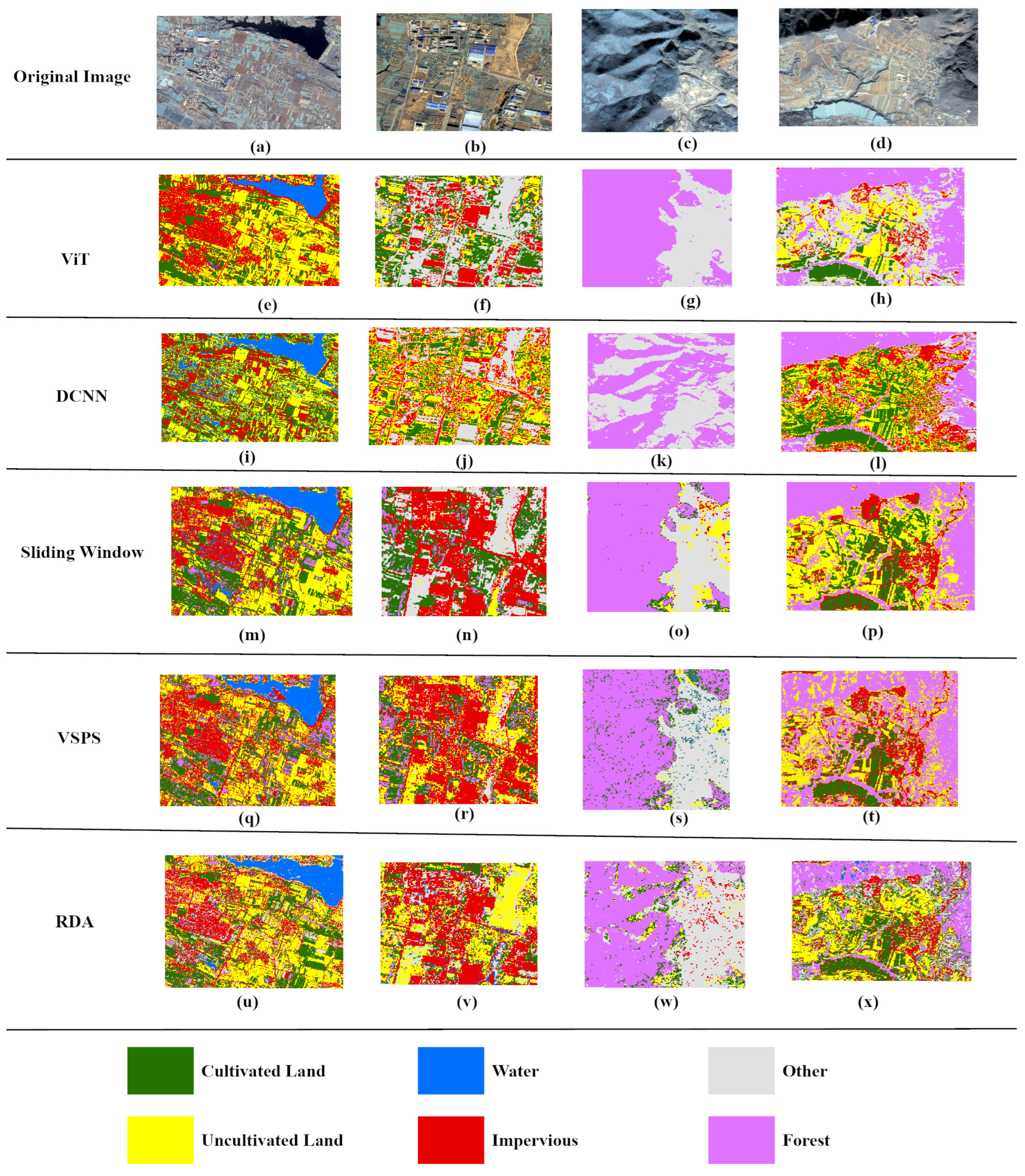
2.11. Comparison with Other Methods

To evaluate the effectiveness of the proposed method, it is compared with other techniques commonly employed for the same objective:

(1)

Deep convolutional neural network (DCNN) [41] can automatically construct the training dataset and execute the classification of multispectral satellite images through deep neural networks.

(2)

The sliding window [13] technique is a prevalent approach for identifying changes in land cover. This method relies on the distinctive or average characteristics of objects within a predefined temporal or spatial window to facilitate the detection of cropland changes [42,43].

(3)

Vegetation–soil–pigment indices and synthetic-aperture radar (SAR) time-series images (VSPS) [44] comprise a multi-temporal indicator-based, large-area mapping framework, which facilitates the automatic identification of active croplands.

(4)

Redundancy analysis (RDA) [17] entails a direct gradient analysis methodology that succinctly captures the linear relationship between the response variable components of a cluster of redundant explanatory variables. This technique can quantify the contribution rate of determinants to the phenomenon of cropland abandonment.

3. Results

3.1. Choosing the Optimal Multiband Composite Image for ViT

The choice of the optimal input image significantly influences the accuracy of the classification outcomes [45]. Therefore, this study assessed the classifier’s performance by including multiple VIs as an additional band for classification, alongside GF-6 single images. The impact of these additions on the final results was examined using accuracy metrics (

Table 3. Illustration of overall accuracy (OA) and F1 score for various combinations of VIs.

VIs	F1 Score	OA
NDVI	0.82	0.82
SAVI	0.83	0.83
TSAVI	0.82	0.83
PVI	0.84	0.84
RTVICore	0.84	0.83
SR	0.84	0.82
NDVI, SAVI, PVI	0.86	0.87
All VIs	0.88	0.91

).

In the context of utilizing a single VI, the lowest accuracy scores were observed when employing GF-6 imagery along with NDVI, resulting in an OA and F1 score of 0.82. Conversely, the highest accuracy values were achieved by incorporating all available VIs, resulting in an OA of 0.91 and an F1 score of 0.88. Based on these findings, the most effective input images for classification involved the integration of all VIs. Subsequently, classification was performed on all nine images from 2019 to 2023.

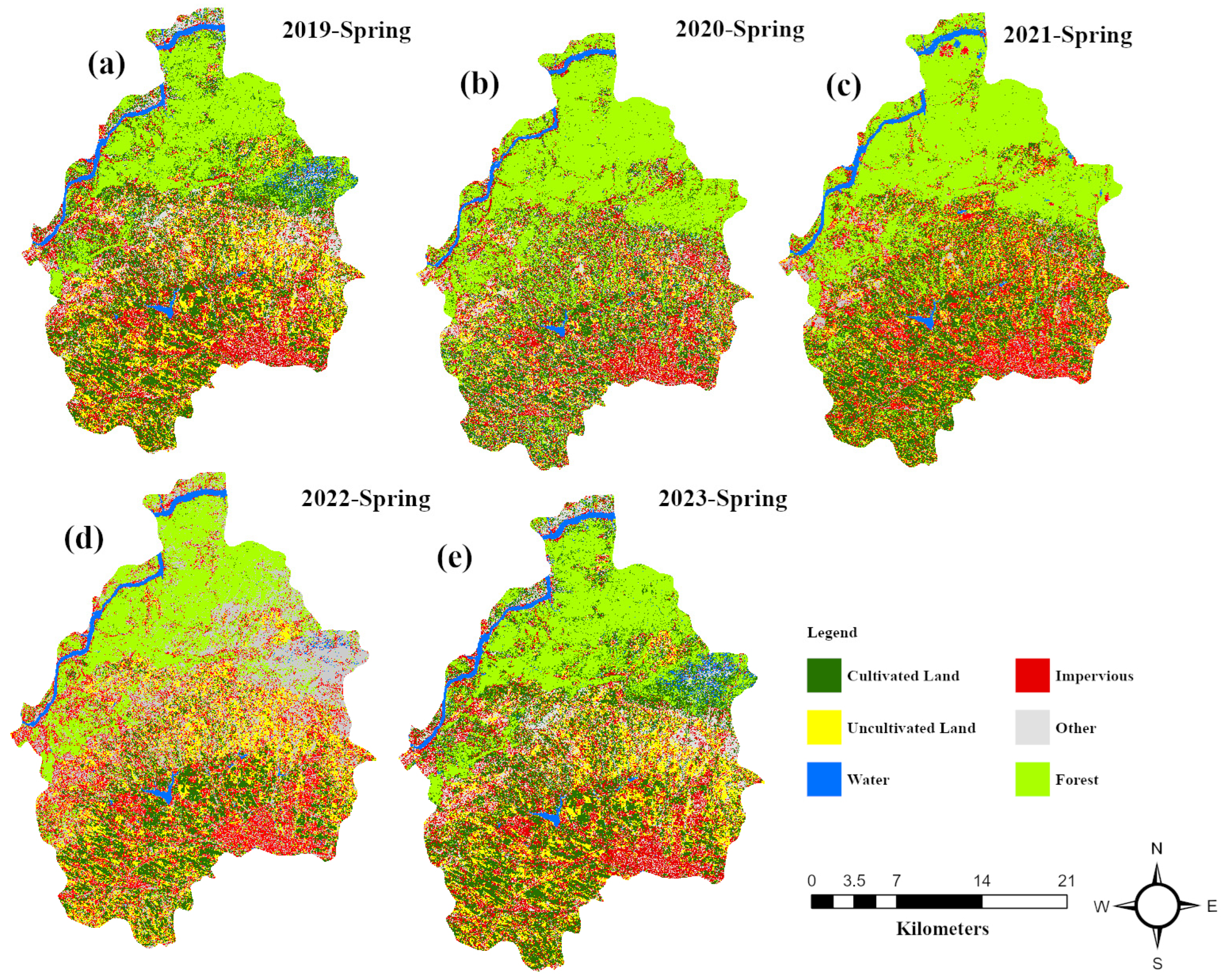
3.2. Inter-Annual Land Use Dynamics and Assessing Classification Accuracy

This study conducts a land cover analysis spanning nine growing seasons, covering the period from 2019 to 2023. This analysis employs multiband composite images of five spring and four fall seasons. Figure 5 illustrates classified areas for each season. The results of the classification revealed seasonal variations in land cover distribution. The order of classified hectares was forest, uncultivated land, other, impervious uncultivated land, and water. The maps were created subsequently for both spring and fall seasons using the classified images (Figure 6 and Figure 7).

Classifier Performance Evaluation

For the final classification assessment, the performance of our classifier was evaluated using a confusion matrix, as illustrated in Figure A1 (Appendix A). During the spring of 2019 to 2023, we observed successful classification of cultivated land in 320, 44, 200, 175, and 91 instances without any false predictions for uncultivated land. However, there were instances where water, forest, and other land cover types were mistakenly labeled as cultivated land. In the fall growing seasons from 2019 to 2022, the confusion matrices showed accurate classification of 184, 164, 171, and 45 instances as cultivated land. Furthermore, we calculated the average values of precision, recall, F1 score, and OA for each image in every growing season (

Table 4. The average values reported for precision, recall, F1 score, and accuracy for the classified images during the spring and fall growing seasons from 2019 to 2023.

	Precision	Recall	F1 Score	OA
Spring 2019	0.9032	0.8858	0.8885	0.9114
Fall 2019	0.8696	0.8945	0.8767	0.9328
Spring 2020	0.8014	0.8790	0.8047	0.9042
Fall 2020	0.8756	0.8574	0.8497	0.9078
Spring 2021	0.8995	0.8998	0.8986	0.9386
Fall 2021	0.8409	0.8877	0.8580	0.9139
Spring 2022	0.8914	0.8888	0.8839	0.9454
Fall 2022	0.8319	0.8982	0.8579	0.9332
Spring 2023	0.8611	0.8784	0.8683	0.9416

). This indicates the successful performance of our classifier in accurately distinguishing between different land covers. However, seasonal variations posed challenges in accurately differentiating between barren land (other classes) and arid mountain regions.

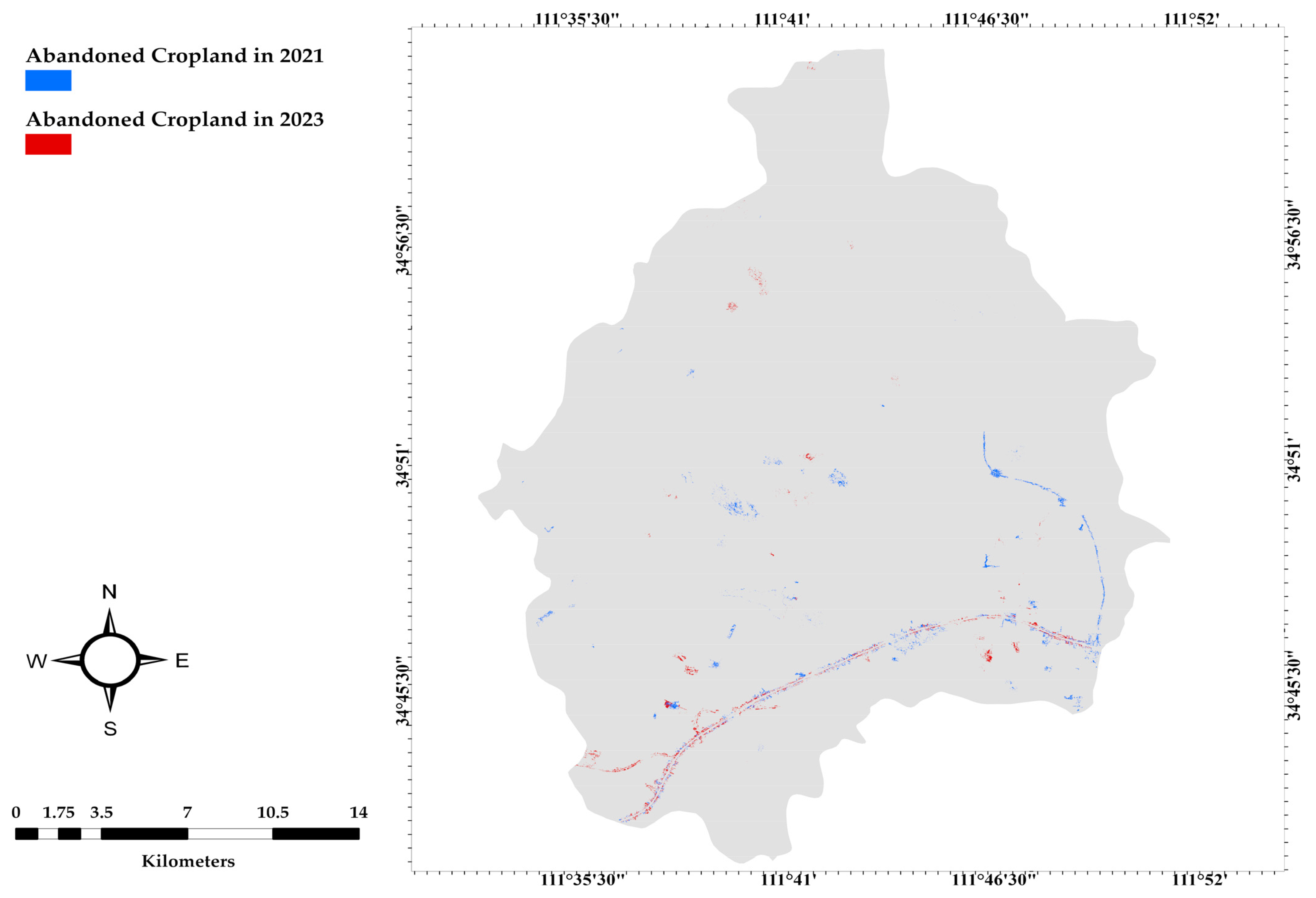
3.3. Spatiotemporal Analysis of Cropland Abandonment: Distribution, Magnitude, Patterns, and Trends

In this study, a spatial and temporal analysis of cropland abandonment was performed, focussing on assessing its distribution, extent, patterns, and evolving trends (Figure 8 and Figure 9). By analyzing multi-temporal satellite imagery, we located and delineated regions where land has been abandoned, providing a detailed spatial distribution across the study area. We merged the results of cultivated and uncultivated land into the category of “cropland” to better understand the changes in land use. We quantified the extent of cropland abandonment by computing the total area of abandoned cropland, which amounted to around 385 hectares. From 2019 to 2021, 270 hectares of cropland experienced abandonment, constituting around 61% of the overall abandoned cropland area. Within this abandoned land, 5 hectares converted to forest, 90 hectares to impervious areas, 109 hectares to various uses like excavation and barren land, and 11 hectares transformed into water bodies.

Similarly, for the period spanning 2021 to 2023, approximately 170 hectares of cropland abandonment were identified, contributing to 33% of the total cropland abandoned area. During this period, 11 hectares were transformed into forest, 27 hectares into impervious areas, 6 hectares into water bodies, and 126 hectares into other uses. Comparing the abandoned cropland area to the total cropland area of 17,541 hectares, we estimated that approximately 2.2% of cropland has been abandoned. This assessment allowed us to understand the magnitude of the issue within the study area. Furthermore, to explore the temporal trends and long-term patterns, we visually verified the changes in abandonment over time using historical satellite images, such as Google Earth Pro, Google Earth Online, and historical maps (Figure 10). This analysis enabled us to identify temporal trends, including increasing or decreasing abandonment rates, and understand long-term patterns and shifts in abandonment behavior.

3.4. Explanatory Variables

In the context of societal transformation from cropland to land abandonment and other land uses, significant changes occur in land use and economic decision making, affecting livelihood strategies [46]. With this understanding, it was hypothesized that the abandonment of cropland would occur due to these dynamics. Taking into account this hypothesis, explanatory variables were selected that were capable of encompassing the spatial attributes and accessibility to the market linked to agricultural activities. Our analysis included variables (Figure 11) such as non-agricultural gross domestic product (GDP) [47], land supply trend and growth, and land prices and growth [48]. Valuable information was obtained regarding non-agricultural GDP, land prices, and land supply trends from 2018 to 2023. Upon analyzing the data, fluctuations were observed in these values, particularly during the years 2021 and 2023. These fluctuations indicated a slight increase in the non-agricultural GDP, land prices, and land supply trends. The observed changes highlighted the dynamic nature of these factors and their influence on the cropland abandonment phenomenon.

3.5. Comparative Analysis of Contemporary Approaches for Cropland Abandonment Detection

This experiment examines how the proposed method influences the enhancement in test accuracy. The results are showcased in

Table 5. Precision, recall, F1 score, and overall accuracy of compared methods.

Methods	Precision	Recall	F1 Score	OA
DCNN [41]	0.7801	0.7221	0.7381	0.9157
Sliding Window [13]	0.6442	0.7959	0.7059	0.9094
VSPS [44]	0.8192	0.8417	0.8270	0.8342
RDA [17]	0.8253	0.8277	0.8263	0.7827
Proposed Method	0.9027	0.8925	0.8977	0.9438

, illustrating the performance of the proposed method on a test set while undergoing training with various methods. Table 5 reveals a clear and distinctive trend that underscores the remarkable effectiveness of our proposed method. Further visual understanding is derived from Figure A2 (Appendix B), showcasing the clarity and interpretability of our results. Every method underwent rigorous testing on our datasets for comparison, demonstrating proficiency in classifying cultivated land and water bodies based on their distinct visual characteristics within the land cover spectrum. Notably, DCNN faced difficulties accurately discerning impervious surfaces from water bodies due to its vulnerability to misclassification in the presence of shadowed building and water pixels (Figure A1).

Land cover classification is a complex task that requires methods capable of distinguishing subtle differences between different land types, like barren lands and uncultivated areas. However, existing approaches like DCNN, sliding window, VSPS, and RDA face challenges in accurately separating barren lands, forests, and uncultivated lands. One main issue is the similarity in spectral signatures between barren lands and uncultivated areas, causing confusion during classification. DCNN’s feature extraction might not handle these subtleties well, while VSPS’s accuracy relies heavily on cropland dataset quality, leading to mixed results. Sliding window methods, while good at local details, might struggle with overall context, and RDA’s complexity might cause confusion between barren and uncultivated classes. However, our proposed method, ViT, outperformed the other methods. It excels at capturing subtle spectral differences and learning to transform input data into a more informative set of features. ViT processes image data sequentially through multiple transformer encoders, extracting detailed features. Its main objective is to extract and learn representations from data rather than making specific decisions or classifications.

3.6. Comparison of Employed VIs

This study presents a meticulous comparison with existing research efforts, evaluating various VIs while emphasizing key parameters, including spectral bands used for calculation, sensitivity to vegetation, robustness to noise, and ease of calculation, as shown in Appendix C (

Table A1. Comparison of vegetation indices utilized in previous studies.

VIs	Spectral Bands	Sensitivity to Vegetation	Robustness to Noise	Ease of Calculation	Studies
Normalized Difference Vegetation Index (NDVI)	R and NIR	High	Moderate	Easy	[61]
Dead Fuel Index (DFI)	R, NIR, and SWIR	Low	Moderate	Moderate	[49]
Normalized Difference Vegetation Index (NDVI)	R and NIR	High	Moderate	Easy
Normalized Difference Water Index (NDWI)	NIR and SWIR	High	Low	High	[17]
Normalized Difference Soil Index (NDSI)	R and SWIR	High	High	Moderate
Enhanced Vegetation Index (EVI2)	R, NIR, and SWIR	Very High	Low	High
Enhanced Vegetation Index (EVI)	R, NIR, and SWIR	Very High	High	Moderate	[13]
Normalized Difference Vegetation Index (NDVI)	R and NIR	High	Moderate	Easy	[21]
Normalized Difference Snow Index (NDSI)	NIR and SWIR	High	High	Easy
Dry Bare-Soil Index (DBSI)	R and NIR	High	High	Moderate	[62]
Enhanced Vegetation Index (EVI2)	R, NIR, and SWIR	Very High	Low	High	[63]
Normalized Difference Vegetation Index (NDVI)	R and NIR	High	Moderate	Easy	[23]
Normalized Difference Vegetation Index (NDVI)	R and NIR	High	Moderate	Easy	[24]
Normalized Difference Vegetation Index (NDVI)	R and NIR	High	Moderate	Easy	[25]
Green Normalized Difference Vegetation Index (GNDVI)	G and NIR	High	Moderate	Easy
Enhanced Vegetation Index (EVI)	R, NIR, and SWIR	Very High	High	Moderate
Normalized Difference Infrared Index (NDII)	R and NIR	High	High	Easy
Normalized Burn Ratio (NBR)	SWIR and NIR	High	Low	Easy
Normalized Difference Building Index (NDBI)	NIR and SWIR	High	Moderate	Easy	[22]
Normalized Difference Vegetation Index (NDVI)	R and NIR	High	Moderate	Easy
Normalized Difference Vegetation Index (NDVI)	R and NIR	High	Moderate	Easy	[18]
Normalized Difference Vegetation Index (NDVI)	R and NIR	High	Moderate	Easy	Proposed VIs
Soil-adjusted Vegetation Index (SAVI)	R and NIR	High	Low	Easy
Modified Soil-adjusted Vegetation Index (MSAVI)	R and NIR	High	High	Easy
Perpendicular Vegetation Index (PVI)	G and NIR	High	High	Easy
Red-Edge Triangulated Vegetation Index (RTVICore)	R, NIR, and SWIR	Very High	High	Moderate
Simple Ratio (SR)	R and NIR	High	Low	Easy

). By carefully considering the spectral bands used in our VIs, the aim was to effectively capture relevant information from the imagery and yield meaningful results for cropland abandonment analysis. Notably, our study demonstrated that the sensitivity of the employed VIs was relatively high compared to the previous research [49], granting us a slight advantage in utilizing unique VIs such as RTVICore and SR. Concerning robustness to noise, our study exhibited a similar pattern to other studies, showcasing high to low robustness for various VIs [13,17,42,43,44,45,46,47,48]. Furthermore, evaluating ease of calculation for the selected VIs allowed us to assess their practicality and efficiency in large-scale cropland abandonment analysis. Although NDVI was the most commonly used index throughout the comparison, our study also incorporated it, creating a valuable symmetry between the previous research and our findings.

On the other hand, EVI, SAVI, and NDWI were notably efficient in capturing the crucial aspects for assessing vegetation [13,17]. In contrast, the VIs, namely SAVI, MSAVI, PVI, RTVICore, and SR, showcase a well-rounded selection. Each of these indices brings unique strengths to the table, enabling a more in-depth analysis of vegetation health and characteristics. SAVI and MSAVI, for instance, have the advantage of correcting NDVI’s sensitivity to soil brightness, making them ideal choices for areas with exposed soil or sparse vegetation cover. Through this rigorous evaluation, our study’s credibility is enhanced, and valuable insights into the effectiveness of the selected VIs in addressing the challenges of cropland abandonment detection are provided.

4. Discussion

4.1. Understanding Spatiotemporal Dynamics and Factors of Cropland Abandonment: Methodological Advancements and Insights

Our study explored the spatial and temporal dynamics of cropland abandonment, considering various factors, including ongoing road construction, excavation activities, the expansion of water bodies, urbanization, and forest expansion. Our contributions and improvements can be summarized in four key aspects: (1) the performance of the classifier, ViT, was enhanced by integrating various VIs and high-resolution GF-2 and GF-6 imagery, enabling more accurate classification of LULC and better estimation of cropland abandonment. Adding multiple VIs, compared to a single or no VI, enhances the capability of capturing diverse vegetation characteristics and mitigates the limitations of relying solely on a single VI. (2). The results showed improvement with adding VIs as an additional parameter to the classifier. (3) Furthermore, our study includes separate analyses for the two annual growing seasons, enabling us to mitigate challenges posed by fuzzy spectral signatures. (4) Including explanatory variables enabled us to understand the underlying factors leading to cropland abandonment. Notably, our findings highlighted the link between transforming agricultural land into alternative land uses and fluctuations in non-agricultural GDP, land prices, and land supply trends. These observations underscore the interconnectedness of various factors in shaping cropland abandonment dynamics.

The results of satellite images revealed a significant increase in cropland abandonment within our study area from 2019 to 2023. Our classifier efficiently classified various land covers, as indicated by precision, recall, F1 score, and accuracy. The total cropland area, comprising both cultivated and uncultivated land, was quantified at 17,541 hectares, with 385 hectares identified as abandoned during this period. Comparing our proposed method to others, its performance stood out prominently. In contrast to our method’s OA of 0.94, DCNN exhibited an OA of 0.91 while encountering difficulties in accurately classifying water. Sliding window, VSPS, and RDA achieved OA values of 0.90, 0.8342, and 0.78, respectively, in comparison to our method. Notably, RDA and VSPS faced challenges distinguishing between barren and uncultivated lands.

4.2. Contrasting Trends in Cropland Abandonment

Unlike Landsat 30 m resolution imagery [3,13,15,17,50,51,52,53,54,55], which may represent multiple land units within a single pixel, the proposed approach allows us to map them separately, reducing the risk of overlooking fluctuations in land cover area and improving the precision of our abandonment assessment. The utilization of GF-6 imagery significantly enhances our capability to discern more intricate spatial patterns within individual agricultural regions, particularly at the county-level scale, which was not fully captured in Zhang et al. and Guo et al.’s [15,50] study investigating cropland abandonment over various provinces. Our study showed that, within Mianchi, a cropland abandonment rate was noted of around 2.2% during the period from 2019 to 2023. These abandonment rates were significantly less than those recorded in mountainous areas of China, where the range was between 14.32% and 27.2% [46,56]. Moreover, compared to global trends, the rates of cropland abandonment in China demonstrated lower levels, even when contrasted with regions such as Eastern Europe, the former Soviet Union, and Chile, where abandonment rates ranged from 16% to 45% [6,57,58,59]. Similarly, they were lower than those observed in Central Asia (13%) [60]. Variations in classification results can be attributed to the resolution of imagery used, considering the county-level scale and the limited study duration from 2019 to 2023. Moreover, the findings of this study spotlight a pronounced concentration of agricultural land abandonment in the study area, predominantly characterized by rugged and hilly terrain.

4.3. Shortcomings and Limitations

The limitations of this research offer significant insights for future studies aimed at advancing our understanding of cropland abandonment dynamics. First, to achieve a more comprehensive understanding of land dynamics, incorporating hyperspectral band imagery to calculate VIs, and incorporating moisture and soil information would greatly enhance the accuracy of analysis. Second, the criteria used in this study to classify land as abandoned were based on two consecutive years of non-cultivation. To better grasp the gradual process of abandonment, it is recommended to extend the duration of the study. Lastly, a comprehensive understanding of the reasons behind farmers’ decisions to abandon their lands remains lacking. Engaging in land surveys and interviews with local farmers could yield invaluable insights into the fundamental drivers of abandonment. Addressing these limitations and considering the suggested future directions would significantly contribute to advancing our knowledge regarding cropland abandonment dynamics.

5. Conclusions

Monitoring the abandonment of cropland is essential for identifying the factors behind land cover alterations and ensuring ecological equilibrium and societal stability. To our current knowledge, this study marks the first of its kind in China, diverging from the conventional approach of temporal land change analysis. Instead, it employs high-resolution GF-6 imagery to reconstruct farmland abandonment within a short timeframe from 2019 to 2023. The incorporation of multiple VIs significantly enhanced the performance of the ViT classifier. The influence of a single VI versus multiple VIs was examined along with GF-6 imagery to establish the most effective multiband composite image for classification. Utilizing a single VI resulted in an OA of up to 82%, while integrating multiple VIs increased accuracy to 92%. For the comprehensive classification encompassing all growing seasons, we evaluated the classifier’s performance using confusion matrices, yielding precision, recall, F1 score, and accuracy measurements. The resultant LULC raster facilitated the identification of cropland changes and abandoned areas’ spatial distribution. Furthermore, the proposed method, compared with existing studies, revealed superior performance. A comparison of VIs also highlighted the advantages of our proposed VIs. Notably, the highest abandonment rate occurred in 2021, representing 1.75% (214 hectares) of the total abandoned area, followed by a 1.17% abandonment rate in 2023 (171 hectares). These research findings provide valuable insights into the dynamics of cropland abandonment and the underlying reasons driving farmers’ decisions to shift towards non-agricultural land uses or sell their lands. Despite extensive research on cropland abandonment worldwide, our understanding of how the increase in urbanization, water bodies, forest expansion, and other socio-economic factors influence agricultural land use dynamics in different regions and over time remains limited. This existing gap in knowledge impedes the efficient enactment of context-specific and precisely targeted policies aimed at preventing unfavorable consequences.

References

1. United Nations. Every Year, 12 Million Hectares of Productive Land Lost, Secretary-General Tells Desertification Forum, Calls for Scaled-up Restoration Efforts, Smart Policies. UN Press: New York, NY, USA. Available online: https://press.un.org/en/2019/sgsm19680.doc.htm (accessed on 3 April 2023).
2. Zakkak, S.; Radovic, A.; Nikolov, S.C.; Shumka, S.; Kakalis, L.; Kati, V. Assessing the Effect of Agricultural Land Abandonment on Bird Communities in Southern-Eastern Europe. J. Environ. Manag. 2015, 164, 171–179. [Google Scholar] [CrossRef]
3. Hou, D.; Meng, F.; Prishchepov, A.V. How Is Urbanization Shaping Agricultural Land-Use? Unraveling the Nexus between Farmland Abandonment and Urbanization in China. Landsc. Urban Plan. 2021, 214, 104170. [Google Scholar] [CrossRef]
4. Zheng, Q.; Ha, T.; Prishchepov, A.V.; Zeng, Y.; Yin, H.; Koh, L.P. The Neglected Role of Abandoned Cropland in Supporting Both Food Security and Climate Change Mitigation. Nat. Commun. 2023, 14, 6083. [Google Scholar] [CrossRef] [PubMed]
5. Li, H.; Song, W. Cropland Abandonment and Influencing Factors in Chongqing, China. Land 2021, 10, 1206. [Google Scholar] [CrossRef]
6. Prishchepov, A.V.; Müller, D.; Dubinin, M.; Baumann, M.; Radeloff, V.C. Determinants of Agricultural Land Abandonment in Post-Soviet European Russia. Land Use Policy 2013, 30, 873–884. [Google Scholar] [CrossRef]
7. Zhong, F.; Li, Q.; Xiang, J.; Zhu, J. Economic Growth, Demographic Change and Rural-Urban Migration in China. J. Integr. Agric. 2013, 12, 1884–1895. [Google Scholar] [CrossRef]
8. Foley, J.A.; DeFries, R.; Asner, G.P.; Barford, C.; Bonan, G.; Carpenter, S.R.; Chapin, F.S.; Coe, M.T.; Daily, G.C.; Gibbs, H.K.; et al. Global Consequences of Land Use. Science 2005, 309, 570–574. [Google Scholar] [CrossRef]
9. Tscharntke, T.; Clough, Y.; Wanger, T.C.; Jackson, L.; Motzke, I.; Perfecto, I.; Vandermeer, J.; Whitbread, A. Global Food Security, Biodiversity Conservation and the Future of Agricultural Intensification. Biol. Conserv. 2012, 151, 53–59. [Google Scholar] [CrossRef]
10. West, P.C.; Gibbs, H.K.; Monfreda, C.; Wagner, J.; Barford, C.C.; Carpenter, S.R.; Foley, J.A. Trading Carbon for Food: Global Comparison of Carbon Stocks vs. Crop Yields on Agricultural Land. Proc. Natl. Acad. Sci. USA 2010, 107, 19645–19648. [Google Scholar] [CrossRef]
11. Houghton, R.A. Revised Estimates of the Annual Net Flux of Carbon to the Atmosphere from Changes in Land Use and Land Management 1850–2000. Tellus B 2003, 55, 378–390. [Google Scholar] [CrossRef]
12. Zhu, X.; Xiao, G.; Zhang, D.; Guo, L. Mapping Abandoned Farmland in China Using Time Series MODIS NDVI. Sci. Total Environ. 2021, 755, 142651. [Google Scholar] [CrossRef] [PubMed]
13. Chen, H.; Tan, Y.; Xiao, W.; He, T.; Xu, S.; Meng, F.; Li, X.; Xiong, W. Assessment of Continuity and Efficiency of Complemented Cropland Use in China for the Past 20 Years: A Perspective of Cropland Abandonment. J. Clean. Prod. 2023, 388, 135987. [Google Scholar] [CrossRef]
14. Khorchani, M.; Gaspar, L.; Nadal-Romero, E.; Arnaez, J.; Lasanta, T.; Navas, A. Effects of Cropland Abandonment and Afforestation on Soil Redistribution in a Small Mediterranean Mountain Catchment. Int. Soil Water Conserv. Res. 2023, 11, 339–352. [Google Scholar] [CrossRef]
15. Zhang, M.; Li, G.; He, T.; Zhai, G.; Guo, A.; Chen, H.; Wu, C. Reveal the Severe Spatial and Temporal Patterns of Abandoned Cropland in China over the Past 30 Years. Sci. Total Environ. 2023, 857, 159591. [Google Scholar] [CrossRef]
16. Liu, B.; Song, W. Mapping Abandoned Cropland Using Within-Year Sentinel-2 Time Series. CATENA 2023, 223, 106924. [Google Scholar] [CrossRef]
17. Hong, C.; Prishchepov, A.V.; Jin, X.; Han, B.; Lin, J.; Liu, J.; Ren, J.; Zhou, Y. The Role of Harmonized Landsat Sentinel-2 (HLS) Products to Reveal Multiple Trajectories and Determinants of Cropland Abandonment in Subtropical Mountainous Areas. J. Environ. Manag. 2023, 336, 117621. [Google Scholar] [CrossRef] [PubMed]
18. Lotfi, P.; Ahmadi Nadoushan, M.; Besalatpour, A. Cropland Abandonment in a Shrinking Agricultural Landscape: Patch-Level Measurement of Different Cropland Fragmentation Patterns in Central Iran. Appl. Geogr. 2023, 158, 103023. [Google Scholar] [CrossRef]
19. Luo, K.; Moiwo, J.P. Rapid Monitoring of Abandoned Farmland and Information on Regulation Achievements of Government Based on Remote Sensing Technology. Environ. Sci. Policy 2022, 132, 91–100. [Google Scholar] [CrossRef]
20. Portalés-Julià, E.; Campos-Taberner, M.; García-Haro, F.J.; Gilabert, M.A. Assessing the Sentinel-2 Capabilities to Identify Abandoned Crops Using Deep Learning. Agronomy 2021, 11, 654. [Google Scholar] [CrossRef]
21. Su, Y.; Wu, S.; Kang, S.; Xu, H.; Liu, G.; Qiao, Z.; Liu, L. Monitoring Cropland Abandonment in Southern China from 1992 to 2020 Based on the Combination of Phenological and Time-Series Algorithm Using Landsat Imagery and Google Earth Engine. Remote Sens. 2023, 15, 669. [Google Scholar] [CrossRef]
22. Wang, Y.; Song, W. Mapping Abandoned Cropland Changes in the Hilly and Gully Region of the Loess Plateau in China. Land 2021, 10, 1341. [Google Scholar] [CrossRef]
23. Feng, H. Individual Contributions of Climate and Vegetation Change to Soil Moisture Trends across Multiple Spatial Scales. Sci. Rep. 2016, 6, 32782. [Google Scholar] [CrossRef] [PubMed]
24. Kocev, D.; Džeroski, S.; White, M.D.; Newell, G.R.; Griffioen, P. Using Single- and Multi-Target Regression Trees and Ensembles to Model a Compound Index of Vegetation Condition. Ecol. Model. 2009, 220, 1159–1168. [Google Scholar] [CrossRef]
25. Praticò, S.; Solano, F.; Di Fazio, S.; Modica, G. Machine Learning Classification of Mediterranean Forest Habitats in Google Earth Engine Based on Seasonal Sentinel-2 Time-Series and Input Image Composition Optimisation. Remote Sens. 2021, 13, 586. [Google Scholar] [CrossRef]
26. Pastick, N.J.; Wylie, B.K.; Wu, Z. Spatiotemporal Analysis of Landsat-8 and Sentinel-2 Data to Support Monitoring of Dryland Ecosystems. Remote Sens. 2018, 10, 791. [Google Scholar] [CrossRef]
27. Mianchi County People’s Government Portal. Available online: http://www.mianchi.gov.cn/ (accessed on 11 June 2023).
28. Gaofen 6. Available online: https://catalyst.earth/catalyst-system-files/help/references/gdb_r/Gaofen-6.html (accessed on 2 February 2023).
29. Rokni, K. Investigating the Impact of Pan Sharpening on the Accuracy of Land Cover Mapping in Landsat OLI Imagery. Geod. Cartogr. 2023, 49, 12–18. [Google Scholar] [CrossRef]
30. Rani, N.; Mandla, V.R.; Singh, T. Evaluation of Atmospheric Corrections on Hyperspectral Data with Special Reference to Mineral Mapping. Geosci. Front. 2017, 8, 797–808. [Google Scholar] [CrossRef]
31. Jönsson, P.; Cai, Z.; Melaas, E.; Friedl, M.A.; Eklundh, L. A Method for Robust Estimation of Vegetation Seasonality from Landsat and Sentinel-2 Time Series Data. Remote Sens. 2018, 10, 635. [Google Scholar] [CrossRef]
32. Dong, J.; Xiao, X.; Chen, B.; Torbick, N.; Jin, C.; Zhang, G.; Biradar, C. Mapping Deciduous Rubber Plantations through Integration of PALSAR and Multi-Temporal Landsat Imagery. Remote Sens. Environ. 2013, 134, 392–402. [Google Scholar] [CrossRef]
33. Kim, B.Y.; Park, S.K.; Heo, J.S.; Choi, H.G.; Kim, Y.S.; Nam, K.W. Biomass and Community Structure of Epilithic Biofilm on the Yellow and East Coasts of Korea. Open J. Mar. Sci. 2014, 4, 286–297. [Google Scholar] [CrossRef]
34. Zhao, B.; Duan, A.; Ata-Ul-Karim, S.T.; Liu, Z.; Chen, Z.; Gong, Z.; Zhang, J.; Xiao, J.; Liu, Z.; Qin, A.; et al. Exploring New Spectral Bands and Vegetation Indices for Estimating Nitrogen Nutrition Index of Summer Maize. Eur. J. Agron. 2018, 93, 113–125. [Google Scholar] [CrossRef]
35. Zhen, Z.; Chen, S.; Qin, W.; Li, J.; Mike, M.; Yang, B. A Modified Transformed Soil Adjusted Vegetation Index for Cropland in Jilin Province, China. Acta Geol. Sin.-Engl. Ed. 2019, 93, 173–176. [Google Scholar] [CrossRef]
36. Baret, F.; Guyot, G. Potentials and Limits of Vegetation Indices for LAI and APAR Assessment. Remote Sens. Environ. 1991, 35, 161–173. [Google Scholar] [CrossRef]
37. Xing, N.; Huang, W.; Xie, Q.; Shi, Y.; Ye, H.; Dong, Y.; Wu, M.; Sun, G.; Jiao, Q. A Transformed Triangular Vegetation Index for Estimating Winter Wheat Leaf Area Index. Remote Sens. 2020, 12, 16. [Google Scholar] [CrossRef]
38. Ryu, J.-H.; Oh, D.; Cho, J. Simple Method for Extracting the Seasonal Signals of Photochemical Reflectance Index and Normalized Difference Vegetation Index Measured Using a Spectral Reflectance Sensor. J. Integr. Agric. 2021, 20, 1969–1986. [Google Scholar] [CrossRef]
39. Dosovitskiy, A.; Beyer, L.; Kolesnikov, A.; Weissenborn, D.; Zhai, X.; Unterthiner, T.; Dehghani, M.; Minderer, M.; Heigold, G.; Gelly, S.; et al. An Image Is Worth 16 × 16 Words: Transformers for Image Recognition at Scale 2021. arXiv 2020, arXiv:2010.11929. [Google Scholar]
40. Han, K.; Xiao, A.; Wu, E.; Guo, J.; Xu, C.; Wang, Y. Transformer in Transformer. Adv. Neural Inf. Process. Syst. 2021, 34, 15908–15919. [Google Scholar]
41. Hu, Y.; Zhang, Q.; Zhang, Y.; Yan, H. A Deep Convolution Neural Network Method for Land Cover Mapping: A Case Study of Qinhuangdao, China. Remote Sens. 2018, 10, 2053. [Google Scholar] [CrossRef]
42. Sheikhy Narany, T.; Aris, A.Z.; Sefie, A.; Keesstra, S. Detecting and Predicting the Impact of Land Use Changes on Groundwater Quality, a Case Study in Northern Kelantan, Malaysia. Sci. Total Environ. 2017, 599–600, 844–853. [Google Scholar] [CrossRef]
43. He, T.; Xiao, W.; Zhao, Y.; Deng, X.; Hu, Z. Identification of Waterlogging in Eastern China Induced by Mining Subsidence: A Case Study of Google Earth Engine Time-Series Analysis Applied to the Huainan Coal Field. Remote Sens. Environ. 2020, 242, 111742. [Google Scholar] [CrossRef]
44. Qiu, B.; Lin, D.; Chen, C.; Yang, P.; Tang, Z.; Jin, Z.; Ye, Z.; Zhu, X.; Duan, M.; Huang, H.; et al. From Cropland to Cropped Field: A Robust Algorithm for National-Scale Mapping by Fusing Time Series of Sentinel-1 and Sentinel-2. Int. J. Appl. Earth Obs. Geoinf. 2022, 113, 103006. [Google Scholar] [CrossRef]
45. Phan, T.N.; Kuch, V.; Lehnert, L.W. Land Cover Classification Using Google Earth Engine and Random Forest Classifier—The Role of Image Composition. Remote Sens. 2020, 12, 2411. [Google Scholar] [CrossRef]
46. Han, Z.; Song, W. Spatiotemporal Variations in Cropland Abandonment in the Guizhou–Guangxi Karst Mountain Area, China. J. Clean. Prod. 2019, 238, 117888. [Google Scholar] [CrossRef]
47. China Economic Data. Available online: https://wap.ceidata.cei.cn/detail?id=lXpY%2Fwo%2FHU8%3D (accessed on 15 May 2023).
48. Land Price in Yuchi County|Land Transaction Data|Land Transaction|Land Bidding and Auction-Where to Choose. Available online: https://www.xuanzhi.com/henan-sanmenxia-mianchi/dijiashuju/at1mint202212maxt202212 (accessed on 15 May 2023).
49. Zhao, X.; Wu, T.; Wang, S.; Liu, K.; Yang, J. Cropland Abandonment Mapping at Sub-Pixel Scales Using Crop Phenological Information and MODIS Time-Series Images. Comput. Electron. Agric. 2023, 208, 107763. [Google Scholar] [CrossRef]
50. Guo, A.; Yue, W.; Yang, J.; Xue, B.; Xiao, W.; Li, M.; He, T.; Zhang, M.; Jin, X.; Zhou, Q. Cropland Abandonment in China: Patterns, Drivers, and Implications for Food Security. J. Clean. Prod. 2023, 138154. [Google Scholar] [CrossRef]
51. Johansen, K.; Phinn, S.; Taylor, M. Mapping Woody Vegetation Clearing in Queensland, Australia from Landsat Imagery Using the Google Earth Engine. Remote Sens. Appl. Soc. Environ. 2015, 1, 36–49. [Google Scholar] [CrossRef]
52. Yusoff, N.; Muharam, F. The Use of Multi-Temporal Landsat Imageries in Detecting Seasonal Crop Abandonment. Remote Sens. 2015, 7, 11974–11991. [Google Scholar] [CrossRef]
53. Jiang, Y.; He, X.; Yin, X.; Chen, F. The Pattern of Abandoned Cropland and Its Productivity Potential in China: A Four-Years Continuous Study. Sci. Total Environ. 2023, 870, 161928. [Google Scholar] [CrossRef]
54. De Castro, P.I.B.; Yin, H.; Teixera Junior, P.D.; Lacerda, E.; Pedroso, R.; Lautenbach, S.; Vicens, R.S. Sugarcane Abandonment Mapping in Rio de Janeiro State Brazil. Remote Sens. Environ. 2022, 280, 113194. [Google Scholar] [CrossRef]
55. Chen, S.; Olofsson, P.; Saphangthong, T.; Woodcock, C.E. Monitoring Shifting Cultivation in Laos with Landsat Time Series. Remote Sens. Environ. 2023, 288, 113507. [Google Scholar] [CrossRef]
56. Chaudhary, S.; Wang, Y.; Dixit, A.M.; Khanal, N.R.; Xu, P.; Fu, B.; Yan, K.; Liu, Q.; Lu, Y.; Li, M. A Synopsis of Farmland Abandonment and Its Driving Factors in Nepal. Land 2020, 9, 84. [Google Scholar] [CrossRef]
57. Baumann, M.; Kuemmerle, T.; Elbakidze, M.; Ozdogan, M.; Radeloff, V.C.; Keuler, N.S.; Prishchepov, A.V.; Kruhlov, I.; Hostert, P. Patterns and Drivers of Post-Socialist Farmland Abandonment in Western Ukraine. Land Use Policy 2011, 28, 552–562. [Google Scholar] [CrossRef]
58. Díaz, G.I.; Nahuelhual, L.; Echeverría, C.; Marín, S. Drivers of Land Abandonment in Southern Chile and Implications for Landscape Planning. Landsc. Urban Plan. 2011, 99, 207–217. [Google Scholar] [CrossRef]
59. Lieskovský, J.; Bezák, P.; Špulerová, J.; Lieskovský, T.; Koleda, P.; Dobrovodská, M.; Bürgi, M.; Gimmi, U. The Abandonment of Traditional Agricultural Landscape in Slovakia—Analysis of Extent and Driving Forces. J. Rural Stud. 2015, 37, 75–84. [Google Scholar] [CrossRef]
60. Löw, F.; Prishchepov, A.V.; Waldner, F.; Dubovyk, O.; Akramkhanov, A.; Biradar, C.; Lamers, J.P.A. Mapping Cropland Abandonment in the Aral Sea Basin with MODIS Time Series. Remote Sens. 2018, 10, 159. [Google Scholar] [CrossRef]
61. Xu, S.; Xiao, W.; Yu, C.; Chen, H.; Tan, Y. Mapping Cropland Abandonment in Mountainous Areas in China Using the Google Earth Engine Platform. Remote Sens. 2023, 15, 1145. [Google Scholar] [CrossRef]
62. Zhao, Z.; Wang, J.; Wang, L.; Rao, X.; Ran, W.; Xu, C. Monitoring and Analysis of Abandoned Cropland in the Karst Plateau of Eastern Yunnan, China Based on Landsat Time Series Images. Ecol. Indic. 2023, 146, 109828. [Google Scholar] [CrossRef]
63. Meijninger, W.; Elbersen, B.; van Eupen, M.; Mantel, S.; Ciria, P.; Parenti, A.; Sanz Gallego, M.; Perez Ortiz, P.; Acciai, M.; Monti, A. Identification of Early Abandonment in Cropland through Radar-Based Coherence Data and Application of a Random-Forest Model. GCB Bioenergy 2022, 14, 735–755. [Google Scholar] [CrossRef]
Figure 1. Enhancing understanding of the research area: (a) overview of China, (b) Henan Province, and (c) study area.
Land 12 01926 g001
Figure 2. Workflow summarizes the process adopted in this research.
Land 12 01926 g002
Figure 3. The entire patch embedding process personalized to the dataset.
Land 12 01926 g003
Figure 4. The comprehensive transformer encoder workflow applied to our dataset.
Land 12 01926 g004
Figure 5. Area calculated in hectares for classified images during the spring and fall growing seasons spanning from 2019 to 2023.
Land 12 01926 g005
Figure 6. LULC classification in 5 spring growing seasons from 2019 to 2023.
Land 12 01926 g006
Figure 7. LULC classification in 4 fall growing seasons from 2019 to 2023.
Land 12 01926 g007
Figure 8. Illustration of (a) cropland area abandoned and rate of abandonment from 2019 to 2021 and (b) cropland area abandoned and rate of abandonment from 2021 to 2023.
Land 12 01926 g008
Figure 9. The spatial distribution of cropland abandonment, where blue-colored areas represent abandoned croplands between 2019 and 2021, while red-colored areas indicate abandoned areas from 2021 to 2023. This visualization provides a clear representation.
Land 12 01926 g009
Figure 10. Visual verification of significant changes in cropland before and after, where blue (abandoned in 2021) indicates (a) impervious surfaces, (b) water, and red (abandoned in 2023) represents (c) excavation, and (d) the transformation into roadside greenways using Google Earth time series images.
Land 12 01926 g010
Figure 11. Explanatory variables: (a) non-agricultural GDP, (b) land prices trend, and (c) land supply trend.
Land 12 01926 g011