Spatiotemporal Distribution and Driving Force Analysis of the Ecosystem Service Value in the Fujiang River Basin, China

Abstract

Identification of spatiotemporal changes in ecosystem service value and their drivers is the basis for ecosystem services management and decision making. This research selects Fujiang River Basin (FJRB) as the area of study, using the equivalent factor method to estimate the ecosystem service value (ESV) variation and characteristics of its spatial distribution. The contributions of the drivers of ecosystem service value and their interactions were also explored using the optimal parameters-based geographical detectors (OPGD) model. The results showed the following: (1) the total ESV increased from 104,891.22 × 10⁶ yuan to 105,032.08 × 10⁶ yuan from 2000 to 2020, and displayed an upward trend from the southeast to northwest; (2) The distribution of ESV showed a strong positive spatial autocorrelation. High ESVs were concentrated upstream of the study region with a higher elevation and vegetation coverage, whereas low values were mainly found in the midstream and downstream regions, where frequent human activity occurs; (3) The elevation of natural factors, HAI and LA of human-social factors, and PEL of landscape pattern factors were the main forces leading to ESV differentiation, and the spatial heterogeneity of ESV in the study area resulted from the synergistic effect of natural factors, human socioeconomic activities, and landscape pattern factors. This research reveals the spatial and temporal patterns and drivers of ecosystem service values in the FJRB, and provides a scientific reference for the establishment of land-use planning and ecological environmental protection mechanisms in this region.

1. Introduction

Ecosystems are the foundation for the survival and development of human society, and the essence of many environmental problems facing humanity is the destruction and degradation of ecosystem functions and services [1]. Ecosystem services (ESs) are the ability of ecosystems to provide tangible or intangible natural products, environmental resources, and ecological public interests to sustain human activities, such as production, consumption, and circulation [2]. The values of ESs are incredibly high and sometimes immeasurable; thus, maintaining ESs is vital for human welfare [3,4]. However, because the socioeconomic system does not adequately elevate ecosystem assets and their value, ESs are considered a free and inexhaustible public service, resulting their overconsumption and ultimately scarcity [5,6]. Therefore, accurately assessing and quantifying ecosystem service value (ESV) and exploring the drivers that influence the spatial heterogeneity of ESV are vital for maintaining human well-being, promoting a healthy development ecosystem, and providing an essential reference for making reasonable ecological protection policies [7].

Currently, the assessment of ESs primarily includes monetary measurements [8], physical measurements [9], and energy-analysis models [10]. Using monetary units to quantify the ESV allows it to be aggregated and compared across ecosystems. The evaluation findings can also be quickly incorporated into the national accounting system, which is essential for environmental accounting and producing a “green” gross domestic product (GDP) [11]. The main methods for assessing ESV include the market price, travel cost, productivity, and benefit transfer methods [12]. Among them, the benefit transfer method is popular, first proposed by Costanza et al. in 1997. It has the advantages of fast evaluation and low cost of data collection [13]. Based on the global equivalent factor table proposed by Costanza et al. [14], a large number of scholars have evaluated the ESV in different countries and regions [15,16,17]. Moreover, the study by Xie et al. [18] supplemented and revised the equivalent factor method to provide a reference for ESV studies in China based on the view of Costanza et al. [14]; this method combined the current situation of the ecosystem with the economic and social development of China. However, because of the scale effect in the assessment of ESV, existing value equivalent factors can be used at the macro scale, and it is challenging to address the requirements of ESV in a specific region [19]. In particular, if the value coefficient corresponds to the actual condition in the research region, the scale effect would directly influence the accuracy of the final ESV assessment [20]. Consequently, an equivalence factor per unit area depending on the current local condition for various sizes and areas must be determined [21].

If the description of the spatial pattern of regional ESs is “knowing what it is”, exploring the driving force on regional ESs is “knowing why”, which is more beneficial in understanding the underlying causes of ecosystem issues and directing local ecological construction [22]. The complex relationship between human and natural ecosystems has attracted the interest of many researchers [23,24,25], but most studies have focused on the relationship between a single factor and ecosystem services [26], or the confirmation of the main influencing factors and their individual effects on ESV [27]. Such studies disregard the combined effects of factors in ESV changes, and lack a systematic perspective to fully comprehend the driving forces on ESV. Sannigrahi et al. noted that the combined effects of the influencing factors were much higher than their individual effects [28]. The diversity and breadth of influencing factors of ESs show that the impact mechanism of ecosystem services is complex. Related studies in China, especially small-scale studies, are not sufficiently detailed. Changes in ESV typically result from the interaction of several causes [16]. To explain the complex ESV variation accurately and comprehensively, the synergistic effect of these drivers should be considered. The OPGD model can quantitatively detect the single-factor driving factor and the multi-factor interaction driving force, which can compensate for the lack of studies on the driving force of ESV. The influencing factors of ESs can be categorized as natural (terrain, climate, soil, biological), socioeconomic (social economy, land-use), and landscape (landscape index, landscape structure) aspects. Regarding natural factors, topography indirectly regulates soil retention, water supply capacity, and crop production capacity by influencing ecological conditions such as the surface’s temperature, the intensity of light, and precipitation [29]. Climate directly regulates hydrothermal conditions and influences ESs [30]. Soil is the background ecological element for organisms to grow and inhabit, and its physical and chemical properties significantly impact ESs [31]. Human factors such as land-use type, changes in land-use intensity, and human activities have an impact on the level of ESs [17,32]. Thus, the synergistic effects of drivers from three aspects (nature, human-social, and landscape) should be considered to provide an accurate and comprehensive explanation of complex ESV changes.

The Fujiang River Basin (FJRB) is a significant headwater and ecological shelter upstream of the Yangtze River Basin and a key ecologically functional region in southwestern China, which has important regional security functions such as water connotation, soil conservation, and biodiversity protection [33]. Jeremy Rayner et al. [34] highlighted that as society develops, the link between the ecological environment and socioeconomic development increases, and there is a growing concern for coordinated or “integrated” policy strategies. Therefore, it is crucial to strengthen the study of ESV in the FJRB and identify its drivers to optimize the ecological structure and coordinate ecological protection and socioeconomic development in the Yangtze River basin. At present, there is a lack of research on ecosystem service valuation and driving force in FJRB. The main research objectives of this study are (1) to assess ESV in different periods (2000, 2010, and 2020), (2) to discuss the spatiotemporal differentiation characteristics of the ESV from 2000 to 2020, and (3) to quantify the drivers of spatial differentiation of ESV. The results of the study will enrich the theoretical knowledge of the complex relationship between drivers and ecosystem services, and provide a theoretical basis for decision making on the regulation of ecosystem functions, the construction of ecological security patterns and the construction of ecological civilization in the FJRB.

2. Materials and Methods

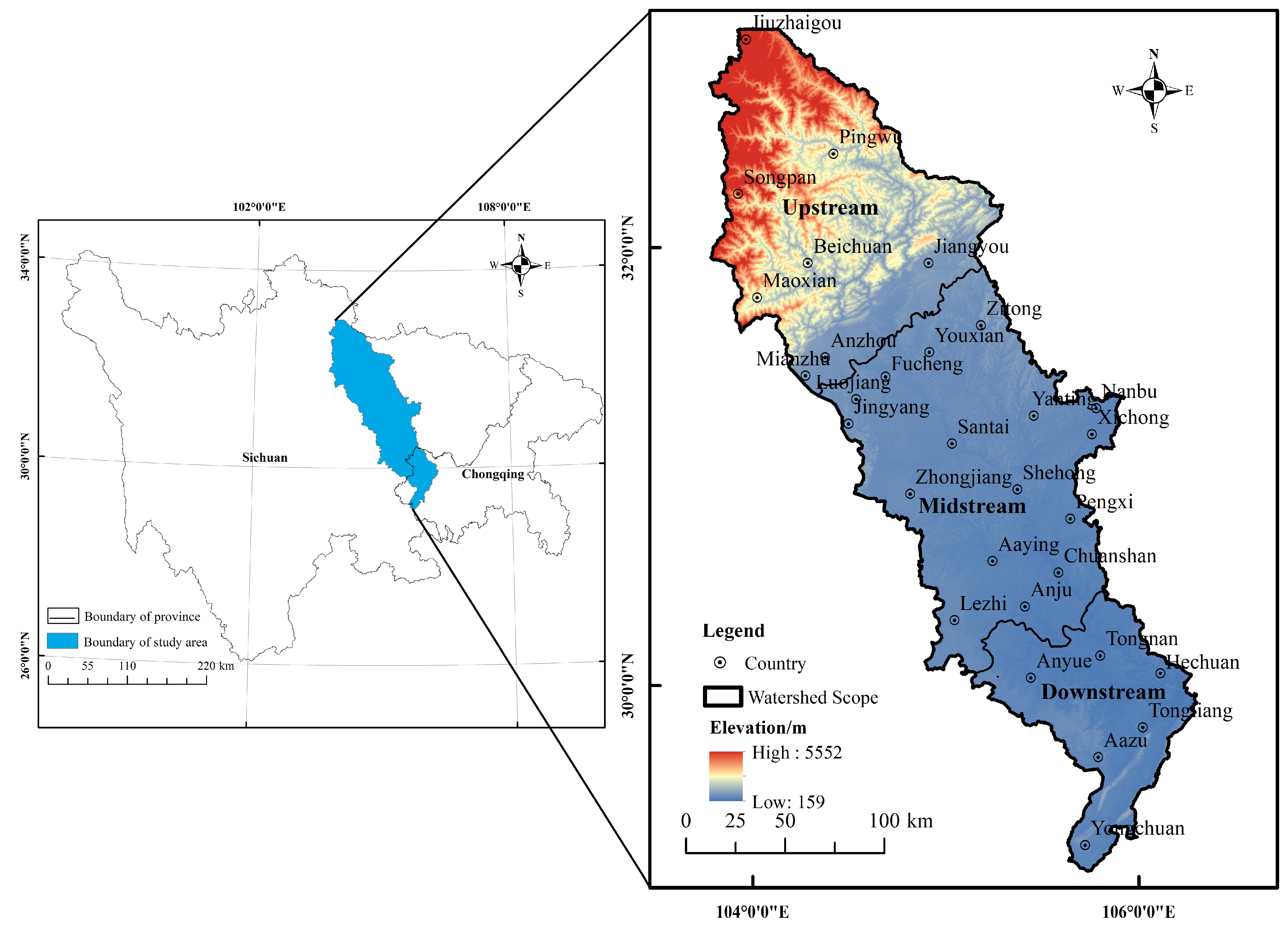
2.1. Study Area

The Fujiang River is the secondary tributary of the Yangtze River and the largest right-bank tributary of the Jialing River. The river is located between 29.10–33.04° N and 103.30–106.30° E, with a total area of 3.92 × 10⁴ km². The multi-year average annual precipitation is >800 mm, with significant spatiotemporal differentiation of precipitation, and the multi-year average annual temperature is >15°. The mean elevation of the FJRB is 986.7 m (above sea level) (a.s.l), and the average slope is approximately 14° [33]. Mountains and hills dominate the terrain, and the elevation difference in the basin is 5393 m. The ecological protection of the FJRB is critical to the long-term development of the Yangtze River Basin (Figure 1).

2.2. Data Source

The LULC data for the three periods in 2000, 2010, and 2020 were all downloaded from the GlobelLand30 (http://www.globallandcover.com, accessed on 23 May 2022) [35]. Six land-use types were obtained after the “China Land Use/Land Cover Remote Sensing Monitoring data classification system” was used to reclassify each year’s land-use types according to the needs of the research: cultivated land, forest land, grassland, waterbody, construction land, and unutilized land (Figure S1). A total of 4658 grids were created by dividing the study area into 3 km by 3 km finishing nets using ArcGIS 10.5. ESV was calculated in these grids. The other geospatial, meteorological, and socioeconomic data are shown in

Table 1. Data sources and processing.

	Driving Factor	Sources and Time	Processing
Nature factor	Temperature (Tem)	https://www.ncdc.noaa.gov/, accessed on 15 March 2022 (2000, 2010, 2020)	Anusplin interpolation model
	Precipitation (Pre)
	Elevation	https://www.gscloud.cn/, accessed on 18 June 2022	ArcGIS Spatial analysis tool
	Slop
	Soil erosion	https://www.resdc.cn/, accessed on 18 June 2022 (2000, 2010, 2020)
	Difference Vegetation Index (NDVI)
Human-social factors	GDP per land (GDP)	(2000, 2010, 2020)	Kriging method
	Population density (POP)	(2000, 2010, 2020)
	Distance from the road (DFR)	https://www.webmap.cn/, accessed on 18 June 2022	Euclidean Distance
	Land use intensity (LA)	[36] (2000, 2010, 2020)	$LA=100\times {\displaystyle {\displaystyle \sum }_{i=1}^n}(A_i\times C_i)$
	Human activity intensity (HAI)	[37] (2000, 2010, 2020)	$HAI={\displaystyle {\displaystyle \sum }_{i=1}^n}\frac{A_i{P}_i}{TA}$
Landscape pattern factors	Landscape Division Index (DIVISION)	LULC data (2000, 2010, 2020)	Fragstats software 4.0
	Contagion Index (CONTAG)
	Shannon’s Diversity Index (SHDI)
	Landscape Shape Index (LSI)
	The Proportion of ecological land (PEL)
Statistic data	Total population	Local Bureau of Statistics (2000, 2010, 2020)
	Gross Domestic Product (GDP)
	Total area

.

2.3. Calculation of ESV

Costanza et al. [38] originally suggested measuring global ESV using the equivalent coefficient method as demonstrated in the current study. An equivalent factor value is 1/7 of the market price of food produced per hectare of arable land per year [18,39]. Based on the average grain yield per unit area in the FJRB, as well as the lowest price of the indica rice in Sichuan Provence from 2000 to 2020, the equivalent factor value of ESs in the FJRB was 2122.77 yuan/hm². The calculating formula of ESV is as follows:

$$\mathrm{ESV}={\displaystyle \sum }_{i=1}^m{A}_i\times V{C}_i$$

(1)

$${\mathrm{ESV}}_j={\displaystyle \sum }_{i=1}^m\left(A_i\times V{C}_{jm}\right)$$

(2)

where $A_i \mathrm{and} V{C}_i$ denotes the area and ESV coefficient of landscape type $i$, respectively, ${\mathrm{ESV}}_j$ represents the jth ESV, and $V{C}_{jm}$ represents the ESV coefficient of jth service of landscape type $i$. The ESV coefficient of each land-use type in the FJRB was obtained (

Table 2. ESV coefficients for each land-use type in the FJRB (yuan/hm²).

	Type	Cultivated Land	Forest Land	Grassland	Waterbody	Unutilized Land
Regulating service	Gas regulation	1061.39	7429.70	1698.22	3820.99	0.00
	Climate regulation	1889.26	5731.48	1910.49	36,299.37	0.00
	Hydrological regulation	1273.66	6792.86	1698.22	32,902.94	63.69
	Soil conservation	3099.24	8278.80	4139.40	3629.94	42.46
Supporting service	Waste disposal	3481.35	2780.83	2780.83	38,591.96	21.23
	Maintaining biodiversity	1507.17	6920.23	2313.82	5306.93	721.74
Provisioning service	Food production	2122.77	212.28	636.83	636.83	21.23
	Raw material production	212.28	5519.20	106.14	148.59	0.00
Cultural service	Aesthetic landscape	21.23	2717.14	84.91	11,781.38	21.23
	Total	14,668.34	46,382.52	15,368.86	133,118.91	891.57

).

2.4. ESV Sensitivity Index Analysis

The sensitivity model used in this study calculates the response of ESV to the variety in the value coefficient (VC). The VC for each land-use type was adjusted by 50%, and then the change in ESV as time passed and the level of dependence on the VC were determined [40]. The formula is as follows:

$$\mathrm{CS}=\left|\frac{\left({\mathrm{ESV}}_j-{\mathrm{ESV}}_i\right)/{\mathrm{ESV}}_i}{\left({\mathrm{VC}}_{jf}-{\mathrm{VC}}_{if}\right)/{\mathrm{VC}}_{if}}\right|$$

(3)

where CS is the sensitivity index, ESV is the total ESV, and VC refers to the value coefficient; i and j represent the initial and change values, respectively (adjusted up or down by 50%), and f represents the land-use type. If CS > 1, the ESV is elastic to the VC. If CS < 1, elasticity is lacking. Therefore, the larger the CS, the more critical the accuracy of the ESV index.

2.5. Spatial Heterogeneity Analysis of ESV

Spatial autocorrelation analysis is a method used to determine whether there is a correlation in the spatial distribution of an attribute and to calculate the degree of correlation. It can intuitively express the correlation and spatial heterogeneity of a certain spatial phenomenon [41,42]. The formula is as follows:

$$Moran’sI=n{\displaystyle \sum }_{i=1}^n{\displaystyle \sum }_{j\ne 1}^n{W}_{ij}\left(x_i-\overline{x}\right)\left(x_j-\overline{x}\right)/({\displaystyle \sum }_{i=1}^n{\displaystyle \sum }_{j=1}^n{W}_{ij}){\displaystyle \sum }_{i=1}^n{\left(x_i-x\right)}^2$$

(4)

where n is the number of spatial cells, $x_i$ and $x_j$ are the ESV of the i and j spatial units, respectively, and W_ij is the spatial weight. The interpretation of the local indicators of spatial association (LISA) is detailed in Table S1.

2.6. Driving Factor Index System Construction

In the geographical exploration of spatial differentiation mechanisms, the choice of the driving factor indicators is crucial [43]. Based on the research area’s actual circumstances and the availability of data principle, three categories and 16 factors were screened out, namely, natural factors (Tem, Pre, elevation, slope, soil erosion, and NDVI), human-social factors (DFR, POP, GDP, HAI, and LA), and landscape pattern factors (DIVISION, SHDI, LSI, CONTAG, and PEL). See Table 1 for details.

2.7. The Optimal Parameter-Based Geographical Detectors Model (OPGD)

The Geographical Detector (Geodetector) is a statistical tool for measuring regionally stratified heterogeneity and performing attribution analysis [44,45]. The OPGD model utilized in this research was created with the GD1.10 package of R, and the spatial discretization and the spatial-scale optimization are both types of parameter optimization [46]. In this study, the q-value was used to measure the independent variable X (16 driving factors) affecting the spatial variation of dependent variable Y (ESVs) at zonal levels in the FJRB. The formula is as follows:

$$q=1-\frac{1}{N{\delta }^2}{\displaystyle \sum }_{n=1}^L{N}_h{\delta }_h{}^2$$

(5)

where q is the independent variable (X)’s explanatory power on the dependent variable (Y), ranging from 0 to 1, L is the layer of X, and $N_h$ and ${\delta }_h$ represent the sample size and variable of the ESV in layer h, respectively. The types of interactions are detailed in Table S2.

3. Results

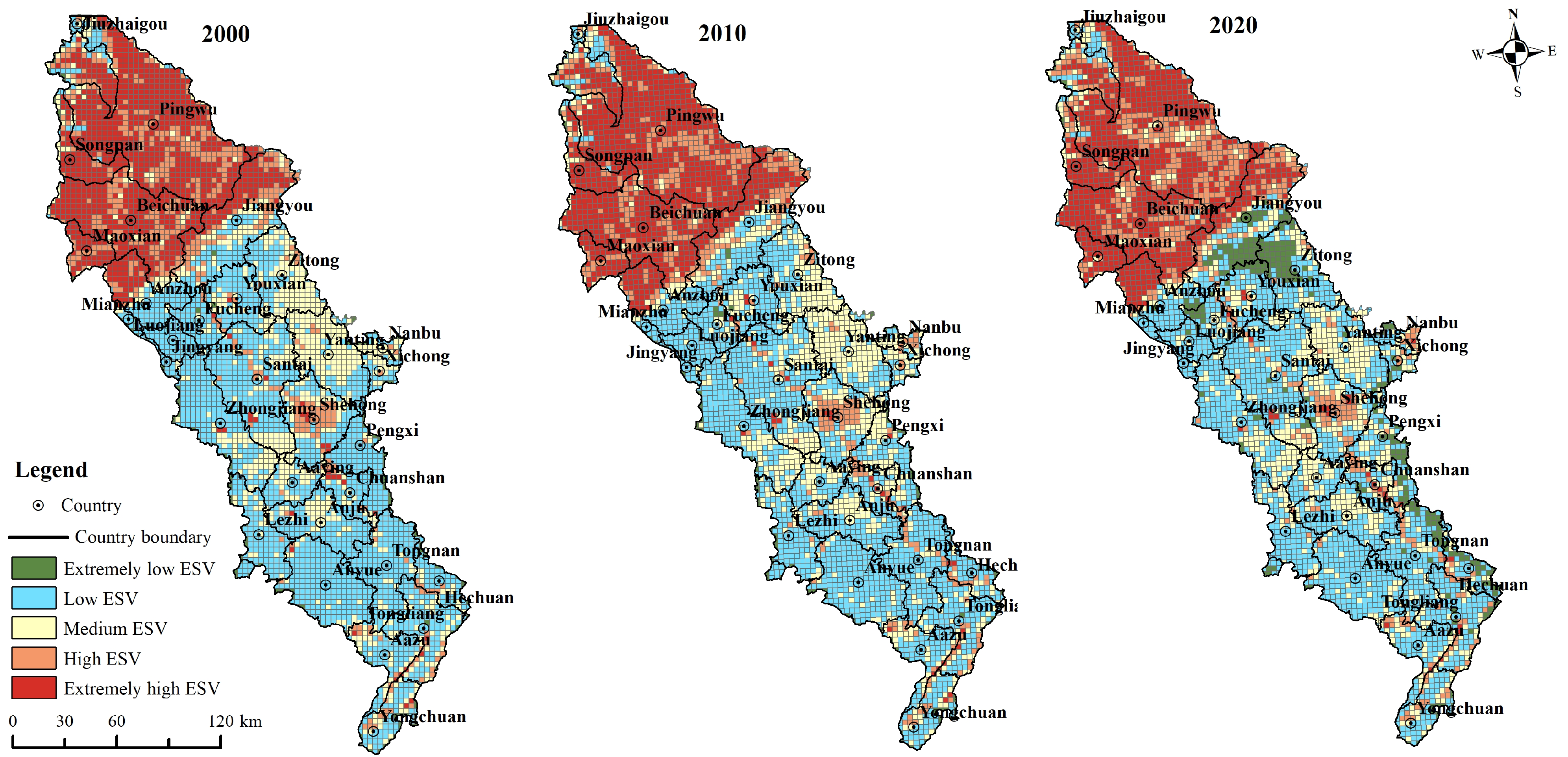
3.1. Analysis of the Spatiotemporal Distribution Characteristics of ESVs in the FJRB

Based on the ESV calculation, the sensitivity index was analyzed according to Formula (3). Considering 2020 as an example, the CS values of the different land-use types were all less than one. Among these, the sensitivity index of forestland was the largest (0.604), while that of farmland, grassland, and waterbody was 0.319, 0.030, and 0.048, respectively. The unused land’s sensitivity index was less than 0.001. Therefore, the ESV was not sensitive to the equivalent coefficient of each land-use type.

The total ESVs of the FJRB in 2000, 2010, and 2020 were 104,891.22 × 10⁶, 105,032.38 × 10⁶, and 105,032.08 × 10⁶ yuan, respectively. From 2000 to 2020, the ESV of the FJRB showed a positive growth state (0.13% growth rate), and the total amount of ESV increased by 140.86 × 10⁶ yuan. Using the natural break classification, the total ESV in the FJRB was divided into five categories (extremely low, low, medium, high, and extremely high).

Table 3. Spatial change tendency of ESV in the FJRB.

Different ESV Grade Zones		Extremely Low	Low	Medium	High	Extremely High
Area (km2)	2000	664.87	17,308.69	7609.63	4533.36	9082.00
	2010	675.50	16,180.56	8434.22	4622.26	9280.00
	2020	2427.85	15,481.19	7656.17	5356.99	8267.35
Change (%)	2000–2010	1.60	−6.52	10.84	1.96	2.18
	2010–2020	259.41	−4.32	−9.22	15.90	−10.91
	2000–2020	265.16	−10.56	0.61	18.17	−8.97

and Figure 2 present the spatial patterns of the ESV from 2000 to 2020. Spatially, the ESV in the FJRB displayed a tendency that increased from southeast to northwest. Among them, the high-value zones are primarily found upstream of the FJRB in the northwest, such as Songpan, Pingwu, and Beichuan, and the highest values of ESV in 2000, 2010, and 2020 were 76.52 × 10⁶, 68.80 × 10⁶, and 75.02 × 10⁶ yuan, respectively. The low-value areas are mainly located in the urban regions of the Fujiang River, such as Youxian, Jingyang, Luojiang, Anyue, and Tongnan.

3.2. Spatial Autocorrelation Analysis of ESVs

Based on ArcGIS 10.5 and the GeoDa 1.18.0 software, and considering the ESV of the FJRB in 2000, 2010, and 2010 as variables, the spatial autocorrelation analysis of ESVs was performed using the queen’s spatial weight method. The Moran’s I values were 0.755, 0.756, and 0.771 in 2000, 2010, and 2020, respectively, and the Z value was greater than 1.96. The research finding shows that the ESV of the FJRB had a strong positive spatial autocorrelation and spatial agglomeration effect from 2000 to 2020; that is, the areas with high ESV tend to be adjacent in space, and the areas with low ESV also have the tendency of adjacent connections in space.

The LISA clustering chart from 2000 to 2020 (Figure 3) shows the low-low agglomeration of ESV in the midstream and downstream of the study region. These regions have a high level of urbanization and relatively concentrated construction land. The government has strengthened the construction and protection of Jiuhaigo, Xuebaodin, Wanglan, and other national nature reserves in the upstream region. The high-high ESV areas are concentrated in these regions. With the intensive production of non-agricultural industries, the lower-low areas of ESV in the northwest of Fucheng, Youxian, south of Anzhou, northwest of Luojiang, Zhongjiang, southwest of Lezhi, east of Pengxi, Anyue, and Tongnan gradually expanded along the urban development axis. The low-high and high-low ESV areas did not change substantially.

3.3. Analysis of the Driving Force of the Spatiotemporal Distribution of ESVs

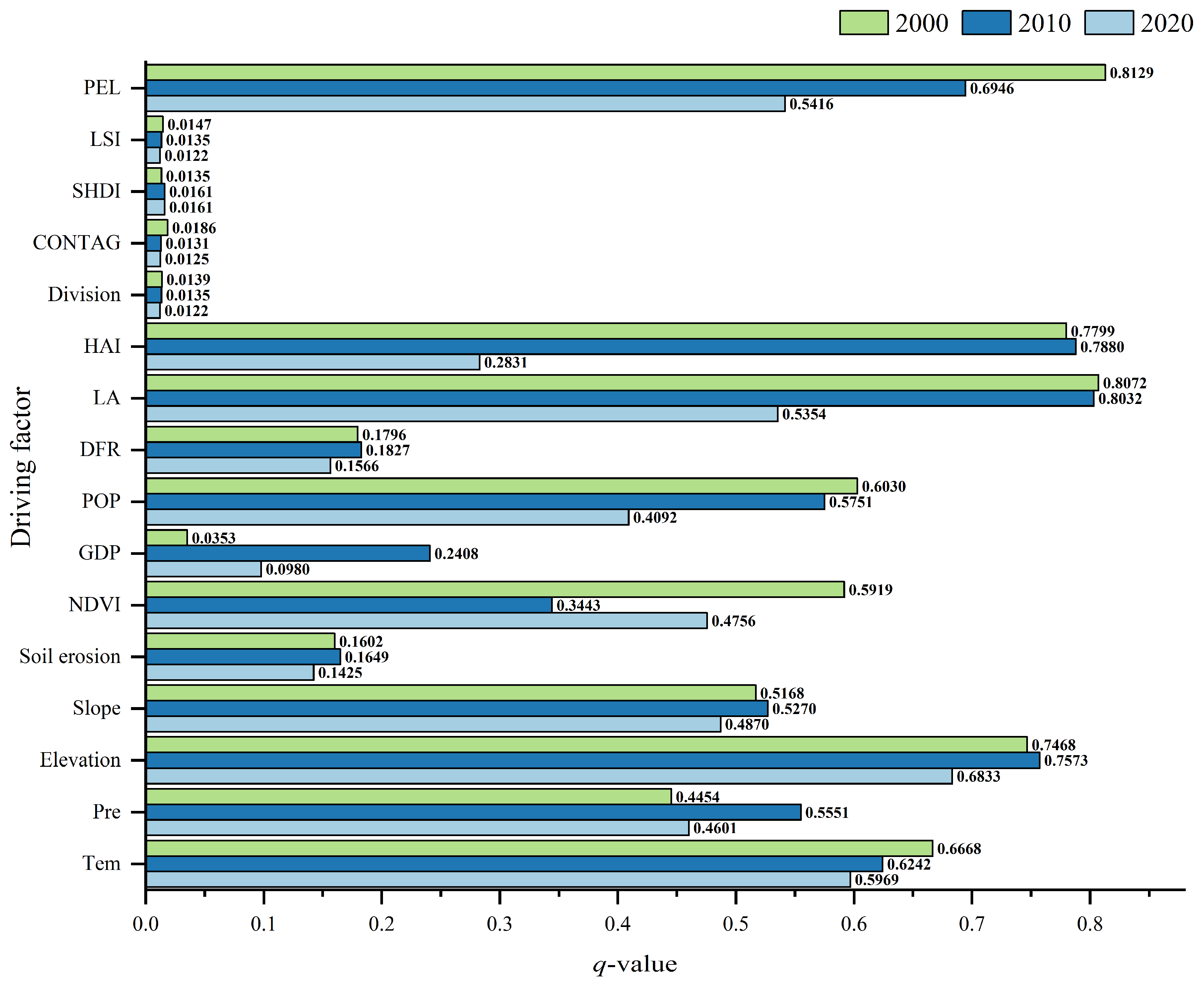
3.3.1. Factor Detector Analysis

The OPGD model was utilized to calculate the driving forces underlying the spatial differentiation of the ESVs in the FJRB from 2000 to 2020 (Figure 4). The spatial differences of the distribution of ESVs in the FJRB were influenced by natural, human-social, and landscape factors. Among them, the spatial variation of ESV in the FJRB in 2000 was most significantly influenced by PEL, HAI, LA, and elevation, all with q-values > 0.74. In 2010, the contributions of factors such as LA, HAL, elevation, PEL, and Tem were less than those in 2000, all with q-values > 0.62. In 2020, the elevation had the biggest contribution to the spatial heterogeneity of ESV in the FJRB, with a q-value of 0.6833. This was followed by a reduced contribution of Tem, PEL, and LA, all with q-values > 0.50. The influencing factors with the highest contribution during 2000–2020 were elevation, PEL, LA, and HAI, with a high explanatory power (q-values > 65%) and significant influence. Second, the influences of POP, Pre, Slope, and NDVI were approximately 40–60%, which are key factors influencing the spatial differentiation of ESVs within the research area. In addition, both the DFR and the effect of soil erosion were greater than 15%, which are minor factors of importance affecting the spatial variation of ESV in the watershed. Finally, the explanatory power of factors such as GDP, LSI, SHDI, DIVISION, and CONTAG was below 10%.

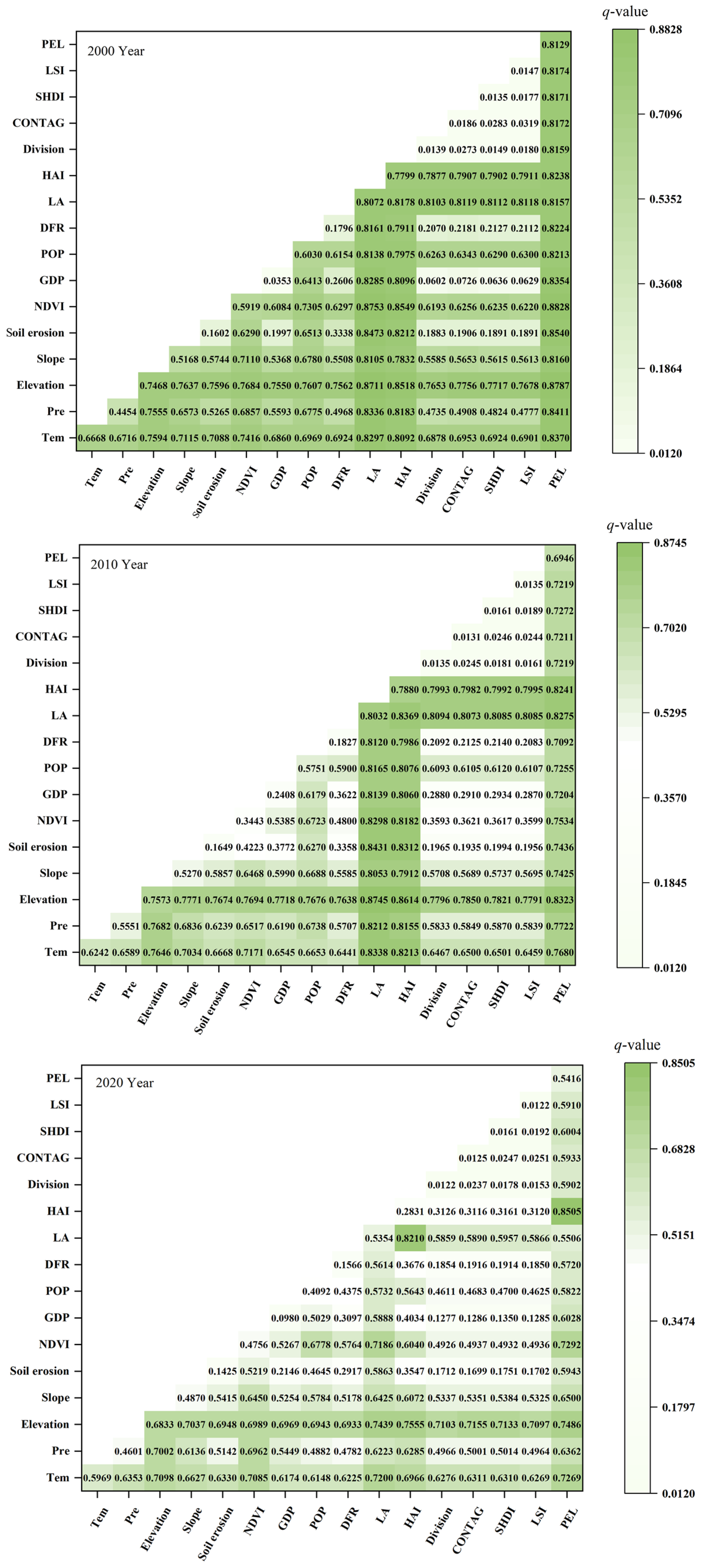
3.3.2. Interaction Detector Analysis

The interaction detector identifies the interaction between different factors on the spatial differentiation of ESV and analyzes whether the dependent variable’s explanatory power increases or decreases (Figure 5). The findings of the interaction for the drivers of the spatial heterogeneity of ESVs in the FJRB show that the interaction of any two of the factors was stronger than the impact of a single factor. The types of the two interactions are primarily nonlinear enhancement interaction-enhancement and two-factor enhancement, indicating that the interaction of multiple factors influences the spatial heterogeneity results of ESVs.

In 2000, the interaction of the PEL and NDVI had the most substantial influence on ESV spatial differentiation, with the highest q-value of 0.8829 for factor interaction detection and an explanatory power close to 90%. The LA, HAI, PEL, and elevation interacting with other arbitrary factors on ESV spatial differentiation in the FJRB were above 80%. In 2010, the spatial variation of ESV in the FJRB was most strongly influenced by the interaction between the LA and elevation, with a q value of factor interaction detection reaching 0.8745. Second, the interaction effects of elevation, LA, HAI, and PEL with other factors were all above 70%, and the interaction effects of Tem, Pre, and slope with other factors were all above 50%. In 2020, the most decisive influence on the spatial variation of ESVs in the FJRB was the interaction between HAI and PEL, with q values as high as 0.8520. The interaction reached more than 75%, including LA ∩ HAI (0.8210) and HAI ∩ elevation (0.7555). Although the q-value of the interactions between the LSI, SHDI, CONTAG, Division, and other factors were under 20%, the results revealed that double factors had a greater effect on ESV spatial difference than single factors (Figure 4).

The results of the analysis indicate that even though the q-values of the interactions between the drivers of spatial differentiation ESV in the study region were decreasing from year to year, the q-values of the interactions were still higher than the q-value of the single factor. The complex coupling between different drivers formed a synergistic enhancement effect that jointly influenced the spatial differentiation effect of ESV in the study region. Furthermore, the interaction results between the PEL and human social factors (HAI, LA) and topographic factors (elevation, slope) showed higher q-values, demonstrating the synergistic enhancement effect of multi-factor interaction on the spatial differentiation of ESV in the FJRB. Therefore, the spatial differentiation of ESV in the FJRB results from the interaction between natural, human-social, and landscape factors, and the interactions between natural and human-social factors are more significant.

4. Discussion

4.1. Analysis of the Driving Force of the Spatiotemporal Distribution of ESVs

ESs have been a focal point in geography, ecology, and other fields, serving as a vital link between human well-being and environmental structure [47]. The value assessment of ESs can provide a reliable basis for assessing ecosystem quality changes, formulating payments for ESs policies, and promoting ecosystem protection and ecological civilization construction [48]. As shown by the elevation map analysis, the northwestern part of the research region is situated in the hilly plateau mountainous area of northwest Sichuan Province. The terrain in this region is primarily mountainous, with considerable differences in vegetation changes, apparent terrain fluctuation, less human activities, and forest land with a high vegetation cover as the primary landscape type in these regions. Therefore, the ESV in the northwest is high. Although the southeast part of the research region is situated in the hilly region of the Sichuan Basin, the terrain is relatively flat, the main land-use types are cultivation and construction land, and human activities are relatively intensive, resulting in a low ESV. Therefore, the ESV in the northwest is higher than in the southeast. This study is consistent with previous research findings on ESV distribution in the southwest and the whole of China [16,18].

In this research, the OPGD model was used to explore the driving mechanism of the spatial heterogeneity of the ESV in the FJRB. It can provide a quantitative analysis of the relative importance of the driving force for the ESV in the study region and identify interactions between factors. In 2000–2020, the factors that explained the strongest q-values of spatial variation in ESV in the FJRB were PEL (0.8130), LA (0.8032), and elevation (0.6832). Among them, the most stable influencing factor was elevation, and the influence was stable at approximately 70% for the period 2000–2020. This is due to the significant elevation difference (the difference between the highest and the lowest elevation is 5393 m), and the apparent topographic relief in the study region. This research also investigated the driving mechanism of ESV spatial differentiation in different regions of the upstream, midstream, and downstream of the FJRB in 2000, 2010, and 2020. The findings showed that the dominant drivers of ESV spatial differentiation characteristics in the area differed more prominently in different regions and periods (Figure 6). During 2000–2020, in the upstream region, the differences in the spatial distribution of ESV were primarily impacted by LA, PEL, HAI, and elevation, all of which had an influence higher than 50%, followed by Tem, Pre, and slope, which had influences of 20–30%; the influence of the remaining factors was less than 10%. In the midstream region, the differences in the spatial distribution of ESV during 2000–2020 were primarily influenced by the factors of PEL, LA, and HAI. The explanatory power of the rest of the factors was less than 10%, indicating that the landscape pattern factors and human-social factors influenced the ESVs distribution in the midstream region. In the downstream region, the spatial variation in ESV during the study period was primarily influenced by PEL, LA, HAI, and elevation. These findings are consistent with the study results. Thus, the spatially heterogeneous distribution of ESV in the study area was influenced by a combination of multiple factors, with natural and human-social factors having the most significant influence, followed by landscape pattern factors.

Overall, based on the OPGD model, 16 drivers were selected from natural, human-social and landscape patterns to investigate the driving force of ESV spatial differentiation, complementing the qualitative and regression analyses that have lacked spatiality in recent years. The result showed that ESV increased with increasing elevation, which is consistent with the studies by Teng et al. in the Qilian Mountains [49]. This is because elevation affects the distribution of temperature, precipitation, and vegetation, which will substantially impact the distribution of ESV. Simultaneously, the interaction of nature and human-social factors might influence the landscape, and the intensity of human activities indirectly changes the distribution and changes of ESVs in the study region. The change in land-use patterns can also modify the spatiotemporal distribution of resources, which further impacts the ecological environment’s structure and function [17]. Among the landscape factors, the contribution rate of the PEL was always the highest, up to 0.8120, and the contribution rate of other landscape factors was low, indicating that the change in landscape pattern would also have an impact on the ecosystem function. Furthermore, changes in landscape patterns affect the processes of material cycling and energy flow in ecosystems and eventually lead to changes in regional ESs via interactions with biotic and abiotic processes [33]. The findings demonstrate that the synergistic interactions of natural, socioeconomic, and landscape pattern factors caused spatial differentiation of ESV in the study region. As a result, decision-making institutions should maximize the allocation of natural resources based on local conditions, control the influence of human social and economic activities on the ecological environment, and adapt the allocation of landscape types when developing future ecosystem management policies.

4.2. Policy Suggestions

Land policy determines the strategic direction of the future development of the region [50], and influences the development of regional urban economic construction [51]. Regional planning should not be guided by a prescriptive view of design, but rather by the rationalization of space and the corresponding approach [51]. This study evaluated the ESVs, analyzed the spatial and temporal variability of ESVs, and quantitatively analyzed the drivers of spatial variability of ESVs in the FJRB, thus providing a scientific reference for urban regional planning and environmental protection policies in the study area and over the whole Yangtze River Economic Zone. Considering the above analysis, the government departments should enhance the protection of nature reserves upstream of the study area and reasonably control the encroachment of human activities on forests and water bodies. We advise that ecological restoration projects should be carried out upstream of the study area, such as comprehensive water environment management, mine restoration, ecological replenishment of forest land, and geological disaster prevention and control; midstream and downstream of the study area, projects such as territorial spatial planning, basic farmland protection planning, and habitat improvements should also be implemented to coordinate the development of an ecological-production-living space. Based on the above analysis, an ecological economy should become mainstream. Abundant water, tourism resources, and high vegetation cover in the study area offer the possibility of this eco-economic model. The ecotourism industry, plantations, three-dimensional agriculture and other organic agricultural practices are all examples of ecological economies that could give the study area its own competitive advantage in the construction of the entire Yangtze River Economic Belt. A change in the economic development model can also reduce the contradiction between ecological protection and economic development, and to a certain extent promote regional sustainable development. Further, to enhance policy feasibility, policy makers should pay closer attention to the effects of drivers on the ESV and tailor them to regional conditions. For example, when formulating ecological restoration policies, a diversified and differentiated coordination strategy should be adopted to weigh and coordinate multiple ecosystem service functions; when formulating territorial spatial planning policies, priority should be given to the differences between local geographical conditions and economic development patterns.

4.3. Limitations and Future Work

In this study, the VC was adjusted to reflect the real condition in the research region accurately, and the ESV in the FJRB was calculated using the ESV equivalent coefficient per unit area. Additionally, using the OPGD model, the explanatory power of each driving force on the spatial differential features of ESV was determined from three aspects (natural, human-social, and landscape pattern). In this study, the OPGD method was used to discretize the dependent variable which improves the reliability and accuracy of applying the geographic detector model. However, the distribution of ESV is influenced by the interaction of several factors and is not simply a positive or negative relationship. Meanwhile, because of the difficulty in obtaining and quantifying the data of some factors, policy factors were not significantly considered. Therefore, more factors should be considered from the viewpoint of ecosystem service stakeholders and human welfare, and quantitative and qualitative analysis methods should be combined to explore the spatiotemporal variation features and driving force of ESV. Furthermore, the ecological compensation mechanism in the FJRB should be further studied to provide a scientific basis for formulating reasonable ecological environmental protection policies in the basin.

5. Conclusions

This research assessed the ESV in the FJRB from 2000 to 2020 using the equivalent coefficient method, and systematically analyzed the spatial and temporal evolution patterns of ESVs. Based on the OPGD model, the driving force of spatial heterogeneity of ESVs in the FJRB are revealed from three aspects (nature, human-social, and landscape pattern). The conclusions are as follows:

(1)

From 2000 to 2020, the total amount of ESV increased by 140.86 × 10⁶ yuan, and the ESV in the FJRB displayed a tendency that increased from southeast to northwest;

(2)

The positive spatial autocorrelation of ESV distribution was significant. The high-value and high-high agglomerated areas were primarily distributed upstream of the FJRB, and the low-value and low-low agglomerated regions were primarily distributed in the midstream and downstream of the FRJB;

(3)

The most significant driving factors were elevation, HAI, LA, and PEL, and the synergistic interactions of natural factors, human activities, and landscape pattern factors contributed to the regional heterogeneity of the ESV in the research region.

In future, to optimize the ecosystem function of the FJRB, it is necessary to adopt differentiated regulation models and strategies based on the impacts of various factors and the interaction characteristics and effects of different factors. These findings serve as a scientific guide for formulating management models with accurate, diversified, and differentiated ecosystem functions.

References

1. Schägner, J.P.; Brander, L.; Maes, J.; Hartje, V. Mapping ecosystem services’ values: Current practice and future prospects. Ecosyst. Serv. 2013, 4, 33–46. [Google Scholar] [CrossRef]
2. Xiao, R.; Lin, M.; Fei, X.; Li, Y.; Zhang, Z.; Meng, Q. Exploring the interactive coercing relationship between urbanization and ecosystem service value in the Shanghai–Hangzhou Bay Metropolitan Region. J. Clean. Prod. 2020, 253, 119803. [Google Scholar] [CrossRef]
3. Li, Y.; Feng, Y.; Guo, X.; Peng, F. Changes in coastal city ecosystem service values based on land use—A case study of Yingkou, China. Land Use Policy 2017, 65, 287–293. [Google Scholar] [CrossRef]
4. Xie, G.; Lu, C.; Leng, Y.; Zheng, D.; Li, S. Ecological assets valuation of the Tibetan Plateau. J. Nat. Resour. 2003, 18, 189–196. [Google Scholar]
5. Daily, G.C.; Söderqvist, T.; Aniyar, S.; Arrow, K.; Dasgupta, P.; Ehrlich, P.R.; Folke, C.; Jansson, A.; Jansson, B.-O.; Kautsky, N. The value of nature and the nature of value. Science 2000, 289, 395–396. [Google Scholar] [CrossRef]
6. Wainger, L.A.; King, D.M.; Mack, R.N.; Price, E.W.; Maslin, T. Can the concept of ecosystem services be practically applied to improve natural resource management decisions? Ecol. Econ. 2010, 69, 978–987. [Google Scholar] [CrossRef]
7. Crossman, N.D.; Burkhard, B.; Nedkov, S.; Willemen, L.; Petz, K.; Palomo, I.; Drakou, E.G.; Martín-Lopez, B.; McPhearson, T.; Boyanova, K. A blueprint for mapping and modelling ecosystem services. Ecosyst. Serv. 2013, 4, 4–14. [Google Scholar] [CrossRef]
8. Costanza, R.; De Groot, R.; Sutton, P.; Van der Ploeg, S.; Anderson, S.J.; Kubiszewski, I.; Farber, S.; Turner, R.K. Changes in the global value of ecosystem services. Glob. Environ. Chang. 2014, 26, 152–158. [Google Scholar] [CrossRef]
9. Gomes, E.; Inácio, M.; Bogdzevič, K.; Kalinauskas, M.; Karnauskaitė, D.; Pereira, P. Future land-use changes and its impacts on terrestrial ecosystem services: A review. Sci. Total Environ. 2021, 781, 146716. [Google Scholar] [CrossRef]
10. Zhan, J.; Zhang, F.; Chu, X.; Liu, W.; Zhang, Y. Ecosystem services assessment based on emergy accounting in Chongming Island, Eastern China. Ecol. Indic. 2019, 105, 464–473. [Google Scholar] [CrossRef]
11. Fu, B.; Lv, Y.; Gao, G. Major research progresses on the ecosystem service and ecological safety of main terrestrial ecosystems in China. Chin. J. Nat. 2012, 34, 261–272. [Google Scholar]
12. King, D.M.; Mazzotta, M.J.; Markowitz, K.J. Ecosystem Valuation. Available online: http://www.ecosystemvaluation.org/default.htm (accessed on 3 February 2023).
13. Liu, Y.; Hou, X.; Li, X.; Song, B.; Wang, C. Assessing and predicting changes in ecosystem service values based on land use/cover change in the Bohai Rim coastal zone. Ecol. Indic. 2020, 111, 106004. [Google Scholar] [CrossRef]
14. Costanza, R.; d’Arge, R.; De Groot, R.; Farber, S.; Grasso, M.; Hannon, B.; Limburg, K.; Naeem, S.; O’neill, R.V.; Paruelo, J. The value of the world’s ecosystem services and natural capital. Nature 1997, 387, 253–260. [Google Scholar] [CrossRef]
15. Chen, T.; Feng, Z.; Zhao, H.; Wu, K. Identification of ecosystem service bundles and driving factors in Beijing and its surrounding areas. Sci. Total Environ. 2020, 711, 134687. [Google Scholar] [CrossRef]
16. Luo, Q.; Zhou, J.; Li, Z.; Yu, B. Spatial differences of ecosystem services and their driving factors: A comparation analysis among three urban agglomerations in China’s Yangtze River Economic Belt. Sci. Total Environ. 2020, 725, 138452. [Google Scholar] [CrossRef]
17. Pan, N.; Guan, Q.; Wang, Q.; Sun, Y.; Li, H.; Ma, Y. Spatial differentiation and driving mechanisms in ecosystem service value of Arid Region: A case study in the middle and lower reaches of Shule River Basin, NW China. J. Clean. Prod. 2021, 319, 128718. [Google Scholar] [CrossRef]
18. Xie, G.; Zhang, C.; Zhang, C.; Xiao, Y.; Lu, C. The value of ecosystem services in China. Resour. Sci. 2015, 37, 1740–1746. [Google Scholar]
19. Hong, Y.; Ding, Q.; Zhou, T.; Kong, L.; Wang, M.; Zhang, J.; Yang, W. Ecosystem service bundle index construction, spatiotemporal dynamic display, and driving force analysis. Ecosyst. Health Sustain. 2020, 6, 1843972. [Google Scholar] [CrossRef]
20. Wu, C.; Chen, B.; Huang, X.; Wei, Y.D. Effect of land-use change and optimization on the ecosystem service values of Jiangsu province, China. Ecol. Indic. 2020, 117, 106507. [Google Scholar] [CrossRef]
21. Rao, Y.; Zhou, M.; Ou, G.; Dai, D.; Zhang, L.; Zhang, Z.; Nie, X.; Yang, C. Integrating ecosystem services value for sustainable land-use management in semi-arid region. J. Clean. Prod. 2018, 186, 662–672. [Google Scholar] [CrossRef]
22. Xue, C.; Zhang, H.; Wu, S.; Chen, J.; Chen, X. Spatial-temporal evolution of ecosystem services and its potential drivers: A geospatial perspective from Bairin Left Banner, China. Ecol. Indic. 2022, 137, 108760. [Google Scholar] [CrossRef]
23. Su, S.; Li, D.; Xiao, R.; Zhang, Y. Spatially non-stationary response of ecosystem service value changes to urbanization in Shanghai, China. Ecol. Indic. 2014, 45, 332–339. [Google Scholar] [CrossRef]
24. Gao, F.; Cui, J.; Zhang, S.; Xin, X.; Zhang, S.; Zhou, J.; Zhang, Y. Spatio-Temporal distribution and driving factors of ecosystem service value in a fragile hilly area of North China. Land 2022, 11, 2242. [Google Scholar] [CrossRef]
25. Su, K.; Wei, D.-Z.; Lin, W.-X. Evaluation of ecosystem services value and its implications for policy making in China–a case study of Fujian province. Ecol. Indic. 2020, 108, 105752. [Google Scholar] [CrossRef]
26. Zhou, D.; Tian, Y.; Jiang, G. Spatio-temporal investigation of the interactive relationship between urbanization and ecosystem services: Case study of the Jingjinji urban agglomeration, China. Ecol. Indic. 2018, 95, 152–164. [Google Scholar] [CrossRef]
27. Song, F.; Su, F.; Mi, C.; Sun, D. Analysis of driving forces on wetland ecosystem services value change: A case in Northeast China. Sci. Total Environ. 2021, 751, 141778. [Google Scholar] [CrossRef]
28. Sannigrahi, S.; Zhang, Q.; Pilla, F.; Joshi, P.K.; Basu, B.; Keesstra, S.; Roy, P.; Wang, Y.; Sutton, P.C.; Chakraborti, S. Responses of ecosystem services to natural and anthropogenic forcings: A spatial regression based assessment in the world’s largest mangrove ecosystem. Sci. Total Environ. 2020, 715, 137004. [Google Scholar] [CrossRef]
29. Zhu, M.; He, W.; Zhang, Q.; Xiong, Y.; Tan, S.; He, H. Spatial and temporal characteristics of soil conservation service in the area of the upper and middle of the Yellow River, China. Heliyon 2019, 5, e02985. [Google Scholar] [CrossRef]
30. Braun, D.; de Jong, R.; Schaepman, M.E.; Furrer, R.; Hein, L.; Kienast, F.; Damm, A. Ecosystem service change caused by climatological and non-climatological drivers: A Swiss case study. Ecol. Appl. 2019, 29, e01901. [Google Scholar] [CrossRef]
31. Wang, Y.; Liu, Z. Vertical distribution and influencing factors of soil water content within 21-m profile on the Chinese Loess Plateau. Geoderma 2013, 193, 300–310. [Google Scholar] [CrossRef]
32. Fu, B.; Zhang, L. Land-use change and ecosystem services: Concepts, methods and progress. Prog. Geogr. 2014, 33, 441–446. [Google Scholar]
33. Zhang, X.; Du, H.; Wang, Y.; Chen, Y.; Ma, L.; Dong, T. Watershed landscape ecological risk assessment and landscape pattern optimization: Take Fujiang River Basin as an example. Hum. Ecol. Risk Assess. Int. J. 2021, 27, 2254–2276. [Google Scholar] [CrossRef]
34. Rayner, J.; Howlett, M. Introduction: Understanding integrated policy strategies and their evolution. Policy Soc. 2009, 28, 99–109. [Google Scholar] [CrossRef]
35. Jun, C.; Ban, Y.; Li, S. Open access to Earth land-cover map. Nature 2014, 514, 434. [Google Scholar] [CrossRef] [Green Version]
36. Zhuang, D.; Liu, J. Study on the model of regional differentiation of land use degree in China. J. Nat. Resour. 1997, 12, 10–16. [Google Scholar]
37. Chen, F.; Ge, X.; Chen, G.; Peng, B. Spatial different analysis of landscape change and human impact in urban fringe. Sci. Geogr. Sin. 2001, 21, 210–216. [Google Scholar]
38. Costanza, R.; Patten, B.C. Defining and predicting sustainability. Ecol. Econ. 1995, 15, 193–196. [Google Scholar] [CrossRef]
39. Fei, L.; Shuwen, Z.; Jiuchun, Y.; Liping, C.; Haijuan, Y.; Kun, B. Effects of land use change on ecosystem services value in West Jilin since the reform and opening of China. Ecosyst. Serv. 2018, 31, 12–20. [Google Scholar] [CrossRef]
40. Kindu, M.; Schneider, T.; Döllerer, M.; Teketay, D.; Knoke, T. Scenario modelling of land use/land cover changes in Munessa-Shashemene landscape of the Ethiopian Highlands. Sci. Total Environ. 2018, 622, 534–546. [Google Scholar] [CrossRef]
41. Xie, H.; Kung, C.-C.; Zhao, Y. Spatial disparities of regional forest land change based on ESDA and GIS at the county level in Beijing-Tianjin-Hebei area. Front. Earth Sci. 2012, 6, 445–452. [Google Scholar] [CrossRef]
42. Huang, C.; Liu, K.; Zhou, L. Spatio-temporal trends and influencing factors of PM2. 5 concentrations in urban agglomerations in China between 2000 and 2016. Environ. Sci. Pollut. Res. 2021, 28, 10988–11000. [Google Scholar] [CrossRef] [PubMed]
43. Liao, J.; Yu, C.; Feng, Z.; Zhao, H.; Wu, K.; Ma, X. Spatial differentiation characteristics and driving factors of agricultural eco-efficiency in Chinese provinces from the perspective of ecosystem services. J. Clean. Prod. 2021, 288, 125466. [Google Scholar] [CrossRef]
44. Wang, J.-F.; Zhang, T.-L.; Fu, B.-J. A measure of spatial stratified heterogeneity. Ecol. Indic. 2016, 67, 250–256. [Google Scholar] [CrossRef]
45. Wang, J.F.; Li, X.H.; Christakos, G.; Liao, Y.L.; Zhang, T.; Gu, X.; Zheng, X.Y. Geographical detectors-based health risk assessment and its application in the neural tube defects study of the Heshun Region, China. Int. J. Geogr. Inf. Sci. 2010, 24, 107–127. [Google Scholar] [CrossRef]
46. Song, Y.; Wang, J.; Ge, Y.; Xu, C. An optimal parameters-based geographical detector model enhances geographic characteristics of explanatory variables for spatial heterogeneity analysis: Cases with different types of spatial data. Giscience Remote Sens. 2020, 57, 593–610. [Google Scholar] [CrossRef]
47. Peng, J.; Hu, X.; Zhao, M.; Liu, Y.; Tian, L. Research progress on ecosystem service trade-offs: From cognition to decision-making. Acta Geogr. Sin. 2017, 72, 960–973. [Google Scholar]
48. Torres, A.V.; Tiwari, C.; Atkinson, S.F. Progress in ecosystem services research: A guide for scholars and practitioners. Ecosyst. Serv. 2021, 49, 101267. [Google Scholar] [CrossRef]
49. Teng, Y.; Zhan, J.; Liu, W.; Chu, X.; Zhang, F.; Wang, C.; Wang, L. Spatial heterogeneity of ecosystem services trade-offs among ecosystem service bundles in an alpine mountainous region: A case-study in the Qilian Mountains, Northwest China. Land Degrad. Dev. 2022, 33, 1846–1861. [Google Scholar] [CrossRef]
50. Shahab, S.; Hartmann, T.; Jonkman, A. Strategies of municipal land policies: Housing development in Germany, Belgium, and Netherlands. Eur. Plan. Stud. 2021, 29, 1132–1150. [Google Scholar] [CrossRef]
51. Hartmann, T.; Jehling, M. From diversity to justice–Unraveling pluralistic rationalities in urban design. Cities 2019, 91, 58–63. [Google Scholar] [CrossRef]
Figure 1. Location of the study area.
Land 12 00449 g001
Figure 2. Total ESV of FJRB from 2000 to 2020.
Land 12 00449 g002
Figure 3. The LISA cluster graph of ESV of FJRB during 2000–2020.
Land 12 00449 g003
Figure 4. Contributions (q statistics) of different factors to ESV variation from 2000 to 2020.
Land 12 00449 g004
Figure 5. Results of interaction detection from 2000 to 2020.
Land 12 00449 g005
Figure 6. Geographical detection q-values of ESVs in the upstream, midstream, and downstream of the FJRB in 2000, 2010, and 2020.
Land 12 00449 g006