Assessing the Relative and Combined Effects of Network, Demographic, and Suitability Patterns on Retail Store Sales

Abstract

Despite challenges associated with acquiring proprietary sales data, there exists a wealth of literature using different types of data (e.g., spending, demographic, geographic) to understand or represent different drivers of retail store sales. We contribute to the spatial analysis of drivers of retail store sales by analyzing the relative influence of road networks, demographic, and suitability variables on retail store sales within the home-improvement sector. Results demonstrate that the inclusion of variables describing the road network pattern is more influential in predicting store sales than demographic and suitability variables with linear models (e.g., ordinary- and partial-least squares regression) as well as with a non-linear mathematical model derived using artificial intelligence. The analysis builds on previous research estimating consumer spending and a big-data suitability analysis for site selection that incorporates spatial interaction models, location quotient, and other unique criteria that are typically used in isolation. The overarching contribution of our results is the demonstration that network patterns can play a critical role in retail store sales, especially when regressions, analogs, and other simple methods for site selection are used.

1. Introduction

Retail strategies are typically highly variable, involving market communications, pricing, and among other factors, product assortment [1]. In contrast, store location is relatively fixed and often represents a long-term investment and commitment (e.g., 99-year lease and building costs). Store location is chosen among many non-controllable elements, for example, demand distribution, market area, accessibility, and competition [2]. While brick-and-mortar retail have historically retained the majority of sales [3], the growing proportion of sales attributed to e-commerce suggests that location decisions are becoming more critical to a retailer’s long-term success in the offline market. However, to survive and succeed, most retailers should be located to not only fulfill market demand but also provide convenient access for in-person customers.

The overarching goal of location–allocation is to simultaneously allocate spatially dispersed (and heterogeneous levels of) demands to potential facility locations to optimize an objective [4]. Specifically, retail site selection aims to maximize profitability by allocating stores as intermediates between central facilities and prospective customers. Traditionally, retail site selection relied on the knowledge and experience of decision-makers using simple checklists or analogs comprising criteria identified at successful stores [5,6,7]. These criteria and similar methods were subjectively defined and composed without objective statistical or spatial analytical approaches [8].

While these simple approaches are frequently adapted, there is an increasing use of analytical methods such as regression, discriminant, and decision tree analyses based on empirical data. Moreover, more complex spatial interaction and optimization methods have been integrated into the site-selection decision-making process. For example, geographic information systems [9], gravity models [10], artificial neural networks [11], spatial interaction models [12], and agent-based modeling [13].

Store accessibility is a critical criterion in consumer patronage and lies at the core of retail location–allocation [4,14,15]. Although the objective in location–allocation is to minimize travel costs between facilities and consumers, accessibility determines the marginal cost related to travel distance [14,16,17]. Factors that impact site accessibility include access to roads or public transport, the level of transport, the quality of ingress and egress, and the availability of parking [14,15]. Practically, a store that provides convenient access can be more attractive to consumers and, consequentially, two neighboring analogous stores can generate significantly different revenue under different degrees of accessibility.

The transportation network, particularly the road network, determines the accessibility of property parcels and the retail stores within. However, the description and use of road network patterns in retail site selection has been subjective and somewhat ambiguous, typically lacking quantitative measurements or convergence on a set of standard measurements [18]. Instead, the pattern of the road network is mostly ignored in retail analyses and used only for distance calculations between points of interest and the generation of service areas. In rare cases, traffic flow across the network is incorporated [19], but a gap remains in our understanding of the contributions of the road network relative to demographic and geographic variables that may influence store sales.

We contribute to the understanding of the factors driving retail store sales by assessing the significance of road network patterns on store sales modeling. Through this effort, we seek to determine if network metrics (i.e., quantitative metrics about network patterns) outperform demographic or suitability variables in retail store sales modeling. As well as the degree to which incorporating road network metrics improves retail store sales modeling. To answer these questions, regression and mathematical models are used to investigate the relative influence of road network patterns on retail revenues.

2. Materials and Methods

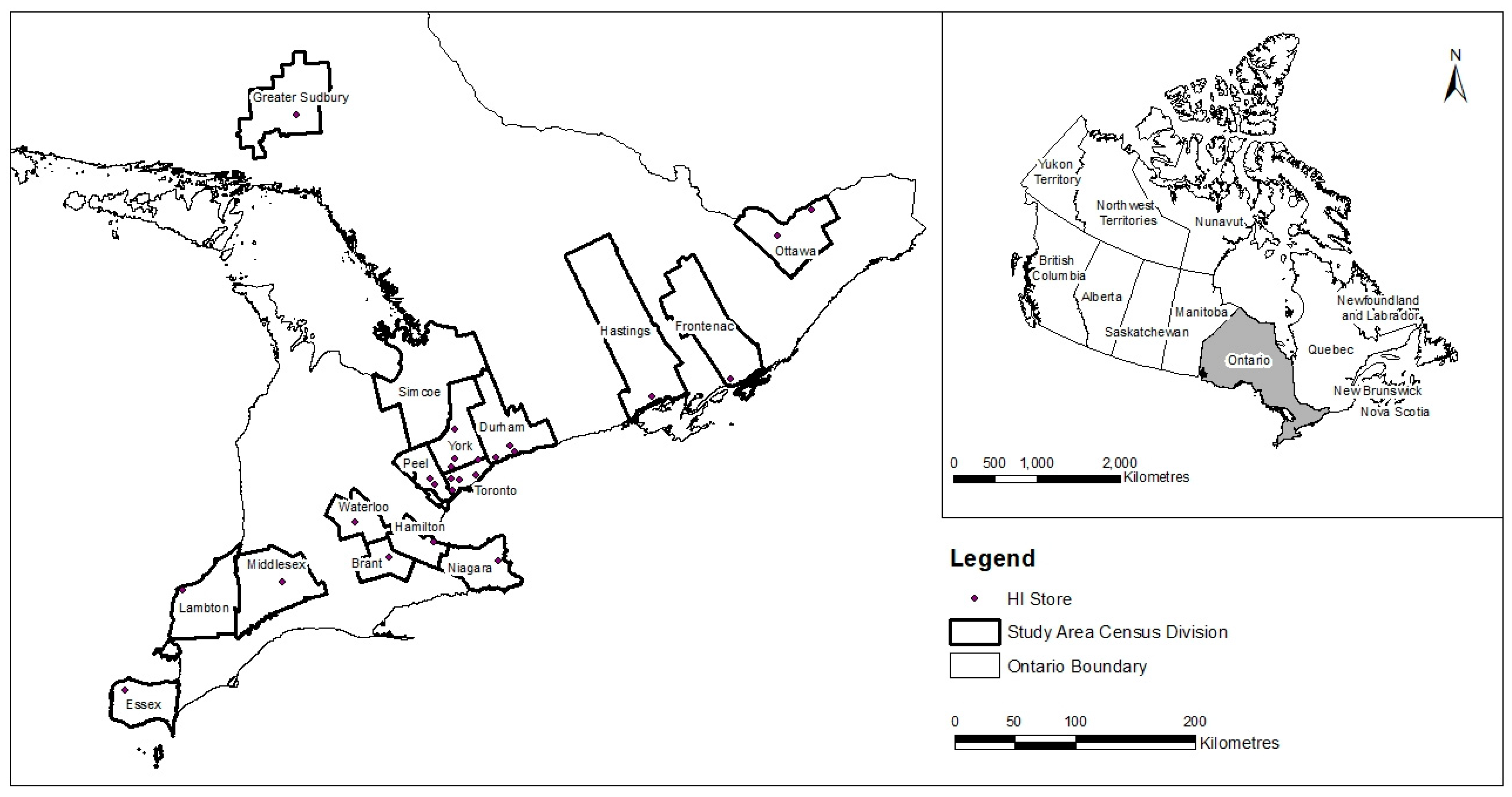
To assess the influence of road network patterns relative to other types of variables typically used in retail site selection, a series of five steps were conducted (Figure 1). While the first step involves the acquisition of data, the second involves calculating a number of metrics or variables that can be evaluated to determine if they have a significant relationship to storing sales data. Calculated metrics and selected variables are scaled to a common range to ensure the units of one variable do not dominate variable selection and model evaluation efforts. Variables are removed from the analysis if they do not show a significant relationship to retail sales (Section 2.3). Then three different types of models are evaluated with different combinations of predictor categories (i.e., network, demographic, and suitability predictors). The models are evaluated using a combination of Akaike’s information criterion, mean squared error, sum of squared errors, R², and the adjusted R².

2.1. Study Area

Ontario is located in east-central Canada, bordering the United States and four of the five Great Lakes (Figure 2). It is the largest province by population in Canada, with about 12.85 million people [20], which is 38.5% of the total population in Canada. Ontario is also one of the largest economic entities in Canada. From 2011 to 2014, Ontario contributed approximately 37% of Canada’s gross domestic product (GDP), with steady growth over the four-year period. Within this context, the retail sector plays an important role in retail trade (North American Industry Classification System (NAICS), 44–45), experiencing an average annual growth rate of 3.5% and a 1.04 billion GDP annual increment from 2012 to 2014. Notably, the annual growth rate of home-improvement stores (identified by NAICS 444) in Ontario from 2012 to 2014 was 4.5%, which is higher than that of the overall retail sector (3.5%). The presented research was conducted in collaboration with a multi-national home-improvement company that occupies a large portion of the Ontario home-improvement retail market.

2.2. Data

Annual store sales data were acquired from twenty-six home improvement retail stores distributed across sixteen census divisions in Ontario. Historical store sales and location information were acquired from an industry collaborator. In addition to these data, road network data for the province were acquired from the Ontario Road Network (2011). A set of road network metrics were used in conjunction with store sales data (2013) to reveal the relationship between road network and store revenue. Meanwhile, demographic information and suitability criteria were developed using data from Statistics Canada, Ontario Ministry of Natural Resources, and Ontario Ministry of Transportation [21,22]. These data were used to derive sets of predictor variables associated with the demographic, suitability, and road network to predict and improve our understanding of the factors driving store sales.

2.2.1. Road Network Metrics

Using a variety of global and local network metrics, the road network pattern was quantified using the following nine network metrics: degree centrality, measure of the number of roads that connect to a node (i.e., intersection); betweenness centrality, the measure of the vitality of a road/crossing in affecting shortest path calculations across a network; load centrality, indicates the influence of crossing over the network using shortest path calculations; entropy, the assortativity of road heterogeneity; fractal dimension, a measure of the form and density distribution of the road network; and density, measures how crowded or dense the road network is within a particular area. Among these network metrics, centrality measurements are local measurements based on individual edges or nodes, while entropy, fractal, and density are global measurements that characterize the structure of a regional road network. To compare the local and global road metrics with point-based store sales, network metrics are summarized at multiple scales for each store location (

Table 1. Road network metrics and statistics.

Spatial Scale	Network Metric
	Global			Local
	Fractal	Entropy	Density	BC	LC	CC	NDC	NLC
Census division	N/A	Entropy	Density	Mean & Standard Deviation
Service area
5-km neighborhood
Community
Adjacent roads		N/A	N/A
Fractal area	Fractal			N/A

Note: BC: betweenness centrality; LC: load centrality; CC: closeness centrality; NDC: node degree centrality; NCC: node closeness centrality; NLC: node load centrality.

).

In addition to the fractal area used in the calculation of the fractal dimension, five spatial scales were used for road network centrality statistics, including census division area, 19-min-drive service area, 5-km neighborhood, community, and adjacent roads. Specifically, 16 census divisions in south-western Ontario were selected for containing stores of interest, and therefore 26 19-min-drive service areas were calculated based on network distance [22], 26 communities were identified by strong network connections ¹, 26 store neighborhoods were created using 5-kilometer buffers around each store, and adjacent roads were identified as roads that provide direct access to a store or the shopping plaza within which a store may reside.

The statistics on network metrics produced 65 variables (Table 1). To reduce the number of network metrics to only those identified as statistically significant, a stepwise regression was performed with a threshold p-value < 0.12. In total, 9 network metrics were selected (

Table 2. Predictor categories (i.e., groups) and the variables within each group, their notation (i.e., symbol), and description.

Group	Variable Name	Symbol	Description
Network	Entropy	ETP	Entropy at community level.
	Closeness centrality mean	CCavg	Mean of closeness centrality at 5 km neighborhood area.
	Closeness centrality standard deviation	CCstd	Standard deviation of closeness centrality at community level.
	Node closeness centrality sum	NCCsum	Sum of node closeness centrality at community level.
	Node closeness centrality mean	NCCavg	Mean of node closeness centrality at community level.
	Betweenness centrality	BC	Standard deviation of betweenness centrality at community level.
	Node load centrality	NLC	Mean of node load centrality at adjacent roads.
	Degree centrality at service area	DC1	Sum of degree centrality at service area.
	Degree centrality at 5 km	DC2	Sum of degree centrality at 5 km.
Demographic	Immigrants	Imm	Total population identified as immigrant in the service area.
	Average dwelling value	DV	Average value of dwelling in the service area.
	Dwelling owner	DO	Count of owned dwellings in the service area.
	Store area	S	Area of a retail store footprint in square feet.
	Dwelling counts	Dc	Count of dwellings in the service area.
	Income over CAD 100,000	Inc	Count of households with income over CAD 100,000.
Suitability	Site maximum slope	b	Maximum value of the parcel’s slope.
	Traffic visibility	v	Defined base on distance from the major highways and the traffic volume.
	Highway accessibility	r	Travel time from a parcel to the nearest highway access point (i.e., ramp).
	Distance to distribution centre	d	The network distance to the nearest distribution centre.
	Market representation	l	Location quotient of a dissemination area.
	Density of competitors	dc	The number of competitors per unit area in the service area.
	Density of retail stores	dr	The number of retailers per unit area in the service area.
	Potential expenditures	ep	Estimated expenditure without competitors in the service area.
	Competitive expenditures	ec	Estimated expenditure with competitors in the service area.

): entropy at the community level (ETP), mean of closeness centrality at a 5 km neighborhood area ($C{C}_{avg}$), standard deviation of closeness centrality at community level $(C{C}_{std}$), sum of node closeness centrality at community level ($NC{C}_{sum}$), mean of node closeness centrality at community level ($NC{C}_{avg}$), standard deviation of betweenness centrality at community level (BC), mean of node load centrality at adjacent roads (NLC), sum of degree centrality at service area ($D{C}_1$), and sum of degree centrality at 5 km ($D{C}_2$).

2.2.2. Demographic Attributes

As part of a larger research project with our industry collaborator, five demographic variables and one site variable were used to model retail store sales (Table 2, [23]). These demographic variables were immigrant population (Imm), average dwelling value ($D_V$), dwelling owner ($D_O$), store area (S), dwelling counts ($D_V$), and households with income over CAD 100,000 (Inc). Demographic data were derived from the 2011 Census and National Household Survey (NHS). Statistics Canada conducts a national survey every five years. In 2011, the long mandatory census was replaced by a combination of a short census and the NHS, which is a detailed voluntary survey. The census data cover topics of population and dwelling counts, age and sex, families, households and marital status, structural type of dwelling and collectives, and language. The NHS data include immigration, income, and housing, among other variables [20].

2.2.3. Suitability Criteria

In collaboration with our home-improvement retail industry partner, a group of their retail experts, comprising a senior vice president and various managers associated with store location decisions, co-identified with the authors and literature, nine sites, and situational criteria for retail site suitability [22]. The site and situational criteria included variables that utilized trade areas, Huff’s model [24], expenditure estimates, and representations of accessibility (Table 2; Appendix A). These criteria were derived from primary data such as the digital elevation model (DEM; Ontario Ministry of Natural Resources), annual average daily traffic (AADT; Ontario Ministry of Transportation), Ontario road network (ORN, Ontario Ministry of Transportation), retail store information, and census data.

Expenditures (i.e., consumer spending) on home improvement products were derived in collaboration with our home-improvement partner and comprised a collection of spending categories from the annual Canadian Survey of Household Spending [21]. These expenditures are summed by census dissemination area (an area comprising 500–700 individuals, which is the smallest census unit in Canada) and are allocated to a potential store location using Huff’s model [24]. The service area for a potential location is generated using a 19-min drive time (the mean network travel time of 23 stores from our sample for which we had data) [22]. Using Huff’s model, two types of expenditures are estimated: potential expenditures (e_p), where expenditures are allocated in the absence of any competition, and competitive expenditures (e_c), where all stores competing for the same expenditure categories are included [22].

2.3. Model Selection

To evaluate the role of network pattern on store sales relative to demographic and suitability predictor variables, a variable selection was first conducted using a ten-fold cross-validation and leaving P out of the cross-validation. Then, with the refined set of predictor variables, three different types of models (linear regression, partial least-square regression, and a mathematical model derived using artificial intelligence) were assessed against store sales data. The predictor categories were used in isolation and combination, for which we use the following nomenclature: network metrics (N), demographic variables (D), and suitability criteria (S) (

Table 3. Categories of predictors and their combination for inclusion in models of sales.

Index	Categories of Predictors
N	Network metrics
D	Demographic variables
S	Suitability criteria
ND	Network metrics and demographic variables
NS	Network metrics and suitability criteria
DS	Demographic variables and suitability criteria
NDS	Network metrics, demographic variables, and suitability criteria

).

During the 10-fold cross-validation, the input dataset is split into ten groups, then one group is selected as the test group, and the remaining nine groups are used as training data. This process is repeated iteratively until all groups have been tested. The leave-P-out cross-validation uses a similar approach but a test group of size p (p = 2 in this study, so it is denoted hereafter as L2O). The test group is selected using an exhaustive enumeration [25]. In this presented research, the L2O produced 325 validation comparisons. The trained models, fit to the test data, were evaluated using the mean of squared error (MSE). A smaller MSE indicates less information loss and better sales modeling. Therefore, variable combinations with small MSE will be selected as model inputs.

The first of the three models assessed was ordinary least squares stepwise regression, which is a semi-automated process for model building and variable subset selection [26]. Stepwise regression is an effective coefficient estimation method in a general linear model when the number of predictors is large, and the data are limited. Backwards stepwise regression was used to determine the significance of variables based on a sequence of t-test and R-squared values; then, a greedy variable selection algorithm was used to remove variables with p-values below 0.1 in backwards eliminations. The resulting model contains only statistically significant variables affecting store sales.

The second model assessed was a partial least squares regression, which reduces the effect of multi-collinearity among variables by projecting predictors and response variables to an orthogonal space. Considering that some of the predictors add little explanatory power to a model, leave-one-out cross-validation was used for component reduction. During the validation process, partial-least squares regression starts from a model with a single predictor, and one observation is omitted from the modeling. Then, the resulting model is fit to the test data to generate residual and R-squared values. The process is repeated until all observations have been omitted once, and then the prediction residual sum of squares and predicted R-squared values are calculated as the average of the test results. Then, another predictor is added to the model, and the cross-validation procedure is repeated until all models (all predictors have been added) have been validated. The model with the lowest prediction residual sum of squares and the highest predicted R-squared would be chosen. Moreover, the variables are rescaled to standardize the deviations to 1; therefore, the results are unbiased regarding the scales of variables.

The final model assessed was a mathematical model generated using Eureqa, an artificial intelligence software originating at the Massachusetts Institute of Technology and the Cornell Lab for Artificial Intelligence (now commercialized through DataRobot). The Eureqa software iteratively tests a wide range of algorithmic building blocks (e.g., addition, subtraction, multiplication, division, trigonometry, and exponential functions) to generate a highly fit model. However, the model is more difficult to interpret than the other approaches because the mathematical components are assembled randomly and propagated using an evolutionary search algorithm rather than being based on theory or conceptual reasoning. Interpretation is further obfuscated because the software, open access at the time, was not open source and has subsequently been acquired for proprietary use.

The models were assessed by their complexity (number of coefficients), information loss (sum of squared errors (SSE), Akaike information criterion (AIC), mean squared error (MSE)), and goodness-of-fit (R-squared and adjusted R-squared). Notably, mathematical modeling may produce non-linear models where the uses of R-squared and adjusted R-squared are controversial [27]. Although they may not reflect the explanatory power of non-linear models, R-squared was calculated to indicate and compare across the generated models.

3. Results

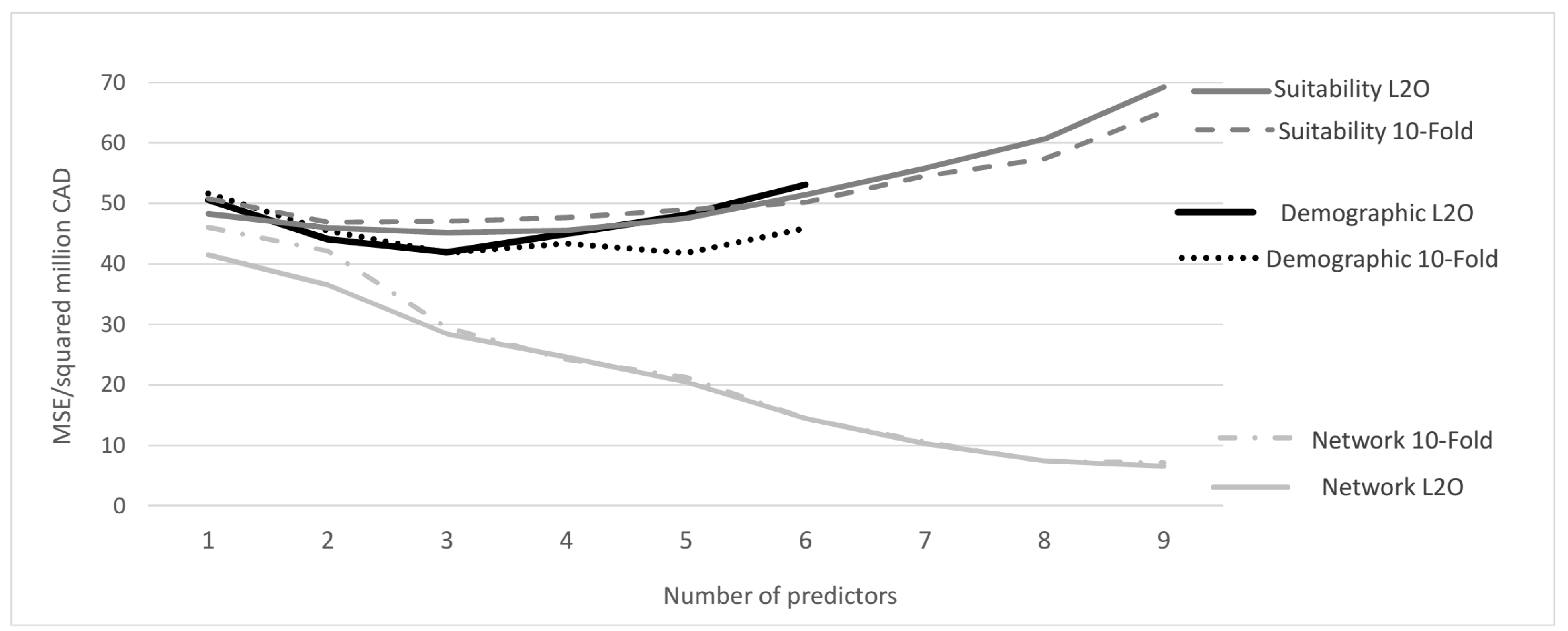
3.1. Model Selection

The performance of the three assessed models varied with the number of predictors included (Figure 3). Therefore, we compare models both with the same number of predictors and overall. Sometimes the two cross-validation schemes (leave-P-out and 10-fold) ranked the same model differently (

Table 4. MSE of the best models of each variable group in cross-validation. Reported in squared million dollars. L2O = leave two out cross-validation, 10-Fold = 10-fold cross-validation.

Number of Variables	Network		Demographic		Suitability
	L20	10-Fold	L20	10-Fold	L20	10-Fold
1	41.52	46.07	50.61	51.65	48.30	50.80
2	36.52	42.17	44.07	45.51	46.01	46.93
3	28.45	29.45	41.95	41.84	45.18	47.07
4	24.61	24.22	45.02	43.41	45.53	47.67
5	20.49	21.27	48.14	41.80	47.54	48.96
6	14.53	14.47	53.13	45.90	51.43	50.19
7	10.31	10.62	-	-	55.8	54.56
8	7.50	7.34	-	-	60.66	57.35
9	6.62	7.19	-	-	69.29	65.21

Note: See Appendix B for more details about predictor selections.

). Our results showed that network metrics strongly affected sales, and models based on network metrics yielded a lower MSE with additional variables and performed better relative to those based on demographic or suitability predictors. In contrast, models based on demographic variables or suitability criteria did not always incur a decrease in MSE with additional variables. For demographic variables, the lowest MSE observed via L2O was from a model with three predictors (4.19 × 10¹³), and the lowest MSE observed via 10-fold was from a model with 5 predictors (4.18 × 10¹³). For suitability criteria, models with 2 (4.60 × 10¹³ via L2O, 4.69 × 10¹³ via 10-Fold), 3 (4.52 × 10¹³ via L2O, 4.71 × 10¹³ via 10-Fold), and 4 (4.55 × 10¹³ via L2O, 4.77 × 10¹³ via 10-Fold) predictors yielded lower MSE than models of other sizes.

Although the MSEs of models with network metrics reduced with an increasing number of predictors, we sought to minimize the number of predictors given our small sample of store sales (n = 26) and maintain comparability with demographic and suitability MSE outcomes. Therefore, model size was limited to two predictors from each of our network, demographic, and suitability categories. In addition to these efforts to yield an unbiased result due to the number of predictors and sample size [28], the best models from L20 and 10-F cross-validations were not always identical (Appendix B). For example, the combination of ETP was recognized as the best in L2O with an MSE of 3.65 × 10¹³ and ranked as the second best in 10-F with an MSE of 4.27 × 10¹³. Considering the overall performance, the model with ETP and CC_std was more stable than the other model and was therefore selected for further analysis. Moreover, Imm and D_v among the demographic variables and e_c and e_p among the suitability criteria outperformed other models in both L2O and 10-F cross-validations.

3.2. Partial Least Squares Regression of Store Sales

A large number of assumptions associated with the data must hold to instill confidence and stability in linear regression results (e.g., independent predictors, uncorrelated residuals with constant variance). Given our small sample size (n = 26) and strong correlations (Pearson correlation coefficient was greater than 0.80 at a significance level of 0.01) among all pairs of demographic and suitability predictors (

Table 5. Pearson correlation coefficient between predictors. *** p < 0.01; ** p < 0.05; * p < 0.1.

Group	Variable	Sales	ETP	CCstd	Imm	DV	eC
Network	ETP	−0.43 **
	CCstd	−0.24	−0.31
Demographic	Imm	−0.17	−0.04	0.183
	DV	0.07	−0.23	0.339 *	0.854 ***
Suitability	eC	−0.11	−0.07	0.081	0.968	0.821 ***
	eP	0.036	−0.16	0.113	0.894 ***	0.824 ***	0.939 ***

; see Appendix C), we assessed the influence of predictors using partial least squares regression, which combines aspects of principal components analysis with multivariate regression to relax the need for independent predictors [29].

The PLS models were established based on isolated or combined predictor categories. Across all models that included network metrics, both entropy at community (ETP) and closeness centrality standard deviation ($C{C}_{std}$) negatively influenced store sales (

Table 6. PLS regression models.

Predictor		PLS-N		PLS-D		PLS-S		PLS-ND		PLS-NS		PLS-DS		PLS-NDS
		Coef	Std Coef.	Coef	Std Coef.	Coef	Std Coef.	Coef	Std Coef.	Coef	Std Coef.	Coef	Std Coef.	Coef	Std Coef.
Network	ETP	−14,832,900	−0.5602					−11,330,900	−0.4280	−12,797,300	−0.4833			−11,038,700	−0.4169
	CCstd	−2.5 × 1012	−0.4130					−3.07 × 1012	−0.5061	−2.52 × 1012	−0.4159			−3.26 × 1012	−0.5385
Demographic	Imm			−12	−0.8576			−10.8624	−0.8042			−12	−0.8640	−7.83958	−0.5804
	DV			45	0.8026			46.1737	0.8304			42	0.7620	45.3097	0.8149
Suitability	eC					0	−1.2417			−0.0071	−1.0266	0	−0.4553	−0.0037	−0.5437
	eP					1	1.2010			1.15981	0.9701	1	0.5653	0.4351	0.3639
Constant		59,523,900	0.0	19,406,816	0.0	2 × 107	0.0	4.3 × 107	0.0	4.7 × 107	0.0	1.4 × 107	0.0	4 × 107	0.0
Coefficients		2		2		2		4		4		4		6
SSR/sqr million		741.12		894.45		916.43		558.86		606.90		815.29		515.65
AIC		811.51		816.40		817.03		808.17		810.31		817.99		810.08
R-Sq		0.34		0.20		0.18		0.50		0.46		0.27		0.54
R-Sq(adj)		0.28		0.14		0.11		0.41		0.36		0.14		0.40

). A high ETP value indicates a high assortativity of road categories, and a low ETP value implies that the road network is dominated by a single category of road segments. At a community level, the standard deviation of closeness centrality ($C{C}_{std}$) indicates the variance of closeness centrality among a road network. A regional road network can be divided into three parts: the “centroid”, which has high closeness centrality; the “periphery”, which has low closeness centrality; and the “connection”, where the variance of closeness centrality is high. A high $C{C}_{std}$ is observed in community road networks that are distributed in the “connection” part of a regional network where the variance of closeness centrality is large; community road networks with small $C{C}_{std}$ values are at either the “centroid” or “periphery” of a regional network where the $C{C}_{std}$ is more stable and has less variance.

Among the demographic variables, dwelling value (D_v) had a positive influence on store sales, and a reduction in estimated sales was affected by the number of immigrants (lmm) within the trade area. These variables align with literature that notes a reduction in investment in renovations when housing value goes below construction costs [30] and higher valued housing stock is more likely to undergo larger and more frequent renovations, and that immigrants to Canada suffer a wage disadvantage relative to non-immigrants [31]. Furthermore, these two variables play a critical role in the geographic distribution of immigrants [32] and disposable income [33].

Our suitability variables (in this case, expenditures) represent the allocated demand for a potential store location [22]. The impacts of competitive expenditure ($e_c$) and potential expenditure without competition ($e_p$) on store sales had different directional effects on store sales. Competitive expenditures had a slightly negative impact on sales, while potential expenditure produced a positive effect on sales.

Comparing the individual predictor category models shows that the model comprising only network metrics (PLS-N) outperformed our demographic and suitability predictors across all evaluation metrics (i.e., lowest SSE, AIC, and highest R² and adjusted R²). Similarly, the combination of network metrics with demographic or suitability predictors (PLS-ND, PLS-NS) outperformed the combination of just demographic and suitability variables (i.e., PLS-DS). While the combination of all three variable categories (PLS-NDS) yielded the lowest SSE and the highest R², it was second to the PLS-ND model, which achieved a lower AIC and adjusted R².

The ordinary least-squares (OLS) regression model (Appendix D) yielded the same direction of signs and magnitudes of coefficients as the PLS models. Similarly, the relative performance, SSE, AIC, and model fit were nearly identical for the individual predictor group models between the OLS and PLS outcomes as well as for any combination of two predictor groups.

3.3. Mathematical Modeling

To investigate the influence of network metrics relative to demographic and suitability predictors on store sales using a non-linear modeling approach, several models were developed using artificial intelligence via evolutionary search routines and random equation construction (Eureqa by Nutonian;

Table 7. Mathematical modeling summary.

	MM-N	MM-D	MM-S	MM-ND	MM-NS	MM-DS	MM-NDS
Number of Coefficients	6	9	9	6	7	7	6
MSE/sqr million	7.62	8.92	13.74	7.88	9.22	6.22	5.16
AIC	787.64	804.54	815.78	788.52	796.37	786.16	777.48
R2	0.82	0.79	0.68	0.82	0.79	0.86	0.88
Search time	2 h 25 min 8 s	2 h 23 min 17 s	2 h 22 min 17 s	19 h 7 min 50 s	19 h 7 min 23 s	19 h 6 min 42 s	48 h 12 min 56 s
Generations	133,584	102,599	99,772	1,176,658	1,174,015	1,156,005	1.45 × 107
Formula evaluations	4.60 × 109	3.50 × 109	3.49 × 109	4.00 × 1010	4.00 × 1010	4.00 × 1010	4.90 × 1011

). The mathematical modeling combines non-linear equation components, and therefore, the number of coefficients produced and used may not correspond to the number of predictors. In our case, with six predictors, the minimum number of coefficients and a maximum of nine coefficients were generated in two models. The selected models are complicated, comprising nested functions, and can contain multiple coefficients applied to the same variable, which makes them difficult to interpret (Appendix B,

Table A6. Mathematical models.

Model	Solution
MM-N	Sales = 59,949,021 + 3,575,175.74850705 × ETP^2 × cos(7,569,808.40234965 × ETP) − 16,006,445.6002844 × ETP − 2,003,466,882,757.61 × CC2 − 3,575,175.52110255 × cos(7,676,585.41034939 × ETP)
MM-D	Sales = 22,834,008.3445785 + 27.8594262541033 × DV + 3,463,461.71205782 × cos(2.05360787074268 × DV) + 6,406,019.97129763 × cos(cos(4.56225343867134 − 2.05360793654371 × DV) − 2.25983877592123 × DV) − 5.94576071728043 × Imm
MM-S	Sales = 47,042,164 + 1.34651074261852 × 10−7 × ec^2 + 0.399358756840768 × ec × sin(4.67160825160463 + 6.24910901352305 × 10−12 × ep^2) − 2.68720110076568 × ec − 4.1233865982514 × 10−12 × ep^2 − 12,260,269.8078034 × sin(4.67160825160463 + 6.24910901352305 × 10−12 × ep^2)
MM-ND	Sales = 98,810,157 + 18.4712932990908 × DV × ETP^3 + −491,820/sin(sin(cos(0.273486737758484 − 18.1794559208219 × ETP^2))) − 48,771,421.1786275 × ETP − 5,343,228,102,286.45 × CC2 − 1.09731557757784 × 10−5 × Imm^2
MM-NS	Sales = 41,593,617/ETP + 3.95138206990593 × ec × ETP + (571,637,654,447,161 + 325,352 × ep)/(ec × ETP) − 87,125,638.0497329 − 5,765,625,660,388.86 × CC2 − 8.18332187565871 × 10−10 × ep × ec × ETP − 3.95138206990593 × ETP × exp(3.95138206990593 × ETP^2)
MM-DS	Sales = 18,377,218 + 31.0449446400918 × DV + 0.417855463557243 × ec + 5,107,267 × sin(sin(0.363700031480952 + 0.255963092026961 × Imm)) − 11.0838224924106 × Imm − 4,892,962.07650244×sin(cos(DV) − 0.249994026057143 × Imm)
MM-NDS	Sales = 56,417,606 + ec + 3,879,411,089,253.75 × ETP × CC2 + 9.18861035767154 × ETP × cos(0.0916227305193614 × Imm)/CC2 − 0.00557917257642006 × ep − 22,626,353.0373718 × ETP − 6,525,672,363,595.11 × CC2

) but also enabled the mathematical models to substantially outperform all OLS and PLS models.

Among the models with isolated predictor groups, the model comprising only network metric predictors (MM-N) yielded the lowest error (MSE), lowest information loss (AIC), and highest goodness of fit. Similar to our PLS results, including network metrics in a non-linear mathematical model in combination with demographic or suitability predictors improved the performance above those predictor categories in isolation, but unlike previous results, they did not surpass the performance of the network metrics in isolation (i.e., MM-N). Furthermore, the combination of demographic and suitability predictors (i.e., MM-DS) outperformed all other models except when all three predictor groups were combined (MM-NDS), which yielded the lowest MSE, lowest AIC, and highest goodness of fit (R²).

4. Discussion

Previous literature has emphasized the critical role that highway access plays in big-box retail success (e.g., [27]). However, to the authors’ knowledge, there is no literature offering a systematic comparison of the influence of road network patterns on store sales relative to demographic and geographic variables that are typically used in site location analyses. Our results demonstrated that the road network pattern, quantified using network metrics, explained a significant amount of variance in store sales. Using three types of models (i.e., ordinary least squares regression [OLS], partial least squares regression [PLS], and an artificial intelligence [AI] model) and three categories of predictor variables (i.e., network, demographic, and suitability), we found that for all but one combination of models and predictor categories (MM-DS) that the inclusion of network metrics increased model performance (R²), reduced error (MSE), and had the lowest Akaike’s information criterion values. These results suggest that future site location and sales prediction efforts should include measurements of network patterns.

Contemporary discussions with the industry suggest that most retail site location analyses are driven by real estate agents, the search for locations that provide an analog between potential store locations and existing and high-performing stores, tacit and experiential knowledge of site acquisition industry experts, and strategic business behavior (e.g., first to market, cut-off competitors). When models are used, they are typically based on simple regression or suitability analyses to ensure transparency and understanding among industry personnel. Our AI model results substantially improved sales forecasting for site selection relative to the OLS and PLS approaches, which contribute to an increasing volume of research that demonstrates the ability of AI models to outperform other approaches, e.g., [34]. The increasing availability of R and python packages, e.g., [35], are increasing the ease at which machine learning and AI approaches can be applied and compared against experiential site-selection knowledge to better locate retail stores to increase accessibility as well as store revenues.

Challenges and Opportunities

Estimating store sales remains a challenge due to those proprietary data not being shared to ensure success among competitors. Our multi-national home improvement company partner was willing to share slightly dated and limited (n = 26) store sales data that corresponded with census and household spending data to investigate the role of network patterns on store sales. While these data were essential, the small sample size limited our number of predictors to six, and likely limited our ability to distill the influence of individual predictors and predictor groups on sales estimates. The small sample size alone could influence collinearity among variables and affect our predictor selection. For example, the correlation between $e_c$ and $e_p$ was 0.94, but when compared using 162,692 estimates from [22], the correlation was 0.72.

In the absence of store sales data, multi-criteria analysis, location–allocation, or consumer exit surveys are used. In the former, predictor (i.e., criteria) weights are derived based using expert opinion in the form of ranking (e.g., modified delphi or collective voting, [36]), using analytical hierarchical process to derive criteria weights by pairwise comparisons among criteria [37] or through the application of equal weights and sensitivity analyses. In location–allocation approaches, a proxy used in lieu of sales (e.g., estimated consumer expenditures) is distributed to stores as a function of distance and store attribute (e.g., size) or location attributes (e.g., presence of other retail and trip-chaining opportunities). However, individual customer location and purchase amounts are typically unknown or, more accurately, are not provided for public use, and therefore, most location–allocation applications lack validation efforts. Customer surveys use receipts or purchase responses along with the time of day and week to estimate sales [38,39,40,41].

The presented research is similarly constrained and cannot share sales data. However, the lack of sales data is an impediment to local economic development and planning as well as limits the advancement of the science of land use change. Therefore, local economic development and planning efforts have been forced to use additional proxy measurements (e.g., location quotient; [42]) to estimate retail opportunities and incentivize companies to locate in a specific area. In urban growth or land use change modeling, which influences both natural (e.g., carbon storage, biodiversity, water quality) and social science (e.g., planning policy impacts on urban morphology, traffic congestion, and human health) and their integration, there remains a near complete void of behavioral representation of commercial actors. While agent-based modeling offers an approach to represent commercial actors and greatly benefits the retail sector, the complete lack of behavioral data influencing retail (and other commercial sectors) location decisions has limited its application to only a couple of efforts [12,40].

In addition to the aforementioned challenges, it could also be argued that our samples were located in highly suitable locations with similar target markets since they are from the same store banner (i.e., brand name). Given that different brands have different target markets, it is expected that some differences will exist among other brands. For example, small format stores are likely to be less affected by our network metrics since their service area is substantially smaller than large format (i.e., big box stores). However, it is worth noting that not all stores within our sample were strong performers. The variation in annual sales spanned a range greater than 29 million Canadian dollars in 2013, with several underperforming stores closed since then.

5. Conclusions

In collaboration with senior management and key personnel associated with market expansion in a multi-national home-improvement company, experiential knowledge suggests that the configuration of the road infrastructure had a direct effect on accessibility and, subsequently, retail store sales. Building on previous research with this partner to estimate consumer expenditures [21] and conduct a multi-scale suitability analysis for retail locations using big data [22], our results demonstrated that the road network pattern was more influential than demographic and suitability predictor variables in estimating store sales using ordinary- and partial-least squares models. In more complex modeling approaches (i.e., mathematical and non-linear modeling), the network metrics outperformed demographic and suitability predictors in isolation, but the combination of only demographic and suitability predictors outperformed any combination of predictor groups that included network metrics. The results of the presented analyses clearly demonstrate that future sales forecasting and site selection should include network metrics.

References

1. Levy, M.; Weitz, A.B.; Grewal, D. Retailing Management; Irwin/McGraw-Hill: New York, NY, USA, 1998. [Google Scholar]
2. Huff, D.L. Parameter Estimation in the Huff Model; ESRI, ArcUser: Redlands, CA, USA, 2003; pp. 34–36. [Google Scholar]
3. Statistics Canada. Table 20-10-0072-01—Retail E-Commerce Sales, Unadjusted, Monthly (Dollars). CANSIM (Database). 2017. Available online: https://www150.statcan.gc.ca/t1/tbl1/en/tv.action?pid=2010007201 (accessed on 5 February 2023).
4. Goodchild, M.F. LACS: A Location-Allocation Mode for Retail Site Selection. J. Retail. 1984, 60, 84–100. [Google Scholar]
5. Clarkson, R.M.; Clarke-Hill, C.M.; Robinson, T. UK supermarket location assessment. Int. J. Retail. Distrib. Manag. 1996, 24, 22–33. [Google Scholar] [CrossRef]
6. O’Malley, L.; Patterson, M.; Evans, M. Retailer use of geodemographic and other data sources: An empirical investigation. Int. J. Retail. Distrib. Manag. 1997, 25, 188–196. [Google Scholar] [CrossRef]
7. Evans, J.R. Retailing in perspective: The past is a prologue to the future. Int. Rev. Retail. Distrib. Consum. Res. 2011, 21, 1–31. [Google Scholar] [CrossRef]
8. Baumgartner, H.; Steenkamp, J.B. Retail Site Selection. SAGE Dict. Quant. Manag. Res. 2011, 31, 271. [Google Scholar]
9. Clarke, I.; Bennison, D.; Pal, J. Towards a contemporary perspective of retail location. Int. J. Retail. Distrib. Manag. 1997, 25, 59–69. [Google Scholar] [CrossRef]
10. Benoit, D.; Clarke, G.P. Assessing GIS for retail location planning. J. Retail. Consum. Serv. 1997, 4, 239–258. [Google Scholar] [CrossRef]
11. Hernandez, T.; Bennison, D. The art and science of retail location decisions. Int. J. Retail. Distrib. Manag. 2000, 28, 357–367. [Google Scholar] [CrossRef]
12. Newing, A.; Clarke, G.P.; Clarke, M. Developing and applying a disaggregated retail location model with extended retail demand estimations. Geogr. Anal. 2014, 47, 219–239. [Google Scholar] [CrossRef]
13. Zhang, J.; Robinson, D. Investigating path dependence and spatial characteristics for retail success using location allocation and agent-based approaches. Comput. Environ. Urban Syst. 2022, 94, 101798. [Google Scholar] [CrossRef]
14. Arentze, T.A.; Borgers, A.W.; Timmermans, H.J. An Efficient Search Strategy for Site-Selection Decisions in an Expert System. Geogr. Anal. 1996, 18, 126–146. [Google Scholar] [CrossRef]
15. Onut, S.; Efendigil, T.; Kara, S.S. A combined fuzzy MCDM approach for selecting shopping center site: An example from Istanbul, Turkey. Expert Syst. Appl. 2010, 37, 1973–1980. [Google Scholar] [CrossRef]
16. Cooper, L. Heuristic methods for location-allocation problems. Siam Rev. 1964, 6, 37–53. [Google Scholar] [CrossRef]
17. Hakimi, S.L. Optimum locations of switching centers and the absolute centers and medians of a graph. Oper. Res. 1964, 12, 450–459. [Google Scholar] [CrossRef]
18. Marshall, S. Streets and Patterns; Institute of Community Studies: London, UK, 2005. [Google Scholar]
19. Luo, S. RTS-GAT Spatial Graph Attention-Based Spatio-Temporal Flow Prediction for Big Data Retailing. IEEE Access 2022, 10, 133232–133243. [Google Scholar] [CrossRef]
20. Statistics Canada. NHS Profile. Retrieved from Statistics Canada. 2011. Available online: https://www150.statcan.gc.ca/n1/en/catalogue/99-004-X (accessed on 5 February 2023).
21. Robinson, D.; Balulescu, A. Comparison of Methods for Quantifying Consumer Spending on Retail using Publicly Available Data. Int. J. Geogr. Inf. Sci. 2018, 32, 1061–1086. [Google Scholar] [CrossRef]
22. Robinson, D.T.; Caradima, B. A multi-scale suitability analysis of home-improvement retail-store site selection for Ontario, Canada. Int. Reg. Sci. Review. 2022, 46, 016001762210924. [Google Scholar] [CrossRef]
23. Balulescu, A.M. Estimating Retail Market Potential Using Demographics and Spatial Analysis for Home Improvement in Ontario; University of Waterloo: Waterloo, ON, Canada, 2015. [Google Scholar]
24. Huff, D.L. A programmed solution for approximating an optimum retail location. Land Econ. 1966, 42, 293–303. [Google Scholar] [CrossRef]
25. Scikit-Learn Developers. Cross-Validation: Evaluating Estimator Performance. 2017. Available online: http://scikit-learn.org/stable/modules/cross_validation.html (accessed on 5 February 2023).
26. Hengl, T.; Heuvelink, G.B.; Stein, A. A generic framework for spatial prediction of soil variables based on regression-kriging. Geoderma 2004, 120, 75–93. [Google Scholar] [CrossRef] [Green Version]
27. Spiess, A.-N.; Neumeyer, N. An evaluation of R2 as an inadequate measure for nonlinear models in pharmacological and biochemical research: A Monte Carlo approach. BMC Pharmacol. 2010, 10, 6. [Google Scholar] [CrossRef] [Green Version]
28. VanVoorhis, C.R.; Morgan, B.L. Understanding power and rules of thumb for determining sample sizes. Tutor. Quant. Methods Psychol. 2007, 3, 43–50. [Google Scholar] [CrossRef]
29. Abdi, H. Partial least squares regression. In Encyclopedia of Measurement and Statistics; Salkind, N., Ed.; Sage Publications: Thousand Oaks, CA, USA, 2007. [Google Scholar]
30. Gyourko, J.; Saiz, A. Reinvestment in the housing stock: The role of construction costs and the supply side. J. Urban Econ. 2004, 55, 238–256. [Google Scholar] [CrossRef]
31. Kaushal, N.; Lu, Y. Recent immigration to Canada and the United States: A mixed tale of relative selection. Int. Migr. Rev. 2015, 49, 479–522. [Google Scholar] [CrossRef] [Green Version]
32. Di Biase, S.; Bauder, H. Immigrant settlement in Ontario: Location and local labour markets. Can. Ethn. Stud. 2005, 37, 114–135. [Google Scholar]
33. Palameta, B. Low Income among Immigrants and Visible Minorities; Cataogue no. 75-001-XIE; Statistics Canada: Ottawa, ON, Canada, 2004. [Google Scholar]
34. Kaneko, Y.; Yada, K. A deep learning approach for the prediction of retail store sales. In Proceedings of the IEEE 16th International Conference on Data Mining Workshops (ICDMW), Barcelona, Spain, 12–15 December 2016; pp. 531–537. [Google Scholar] [CrossRef]
35. Tensorflow Developers. TensorFlow (v2.9.3); Zenodo: online, 2022. [Google Scholar] [CrossRef]
36. Carr, M.H.; Zwick, P.D. Smart Land-Use Analysis: The LUCIS Model Land-Use Conflict Identification Strategy; ESRI, Inc.: Redlands, CA, USA, 2007. [Google Scholar]
37. Saaty, R. The Analytic Hierarchy Process-What and How It Is Used. Math. Model. 1987, 9, 161–176. [Google Scholar] [CrossRef] [Green Version]
38. Applebaum, W. Methods for Determining Store Trade Areas, Market Penetration, and Potential Sales. J. Mark. Res. 1966, 3, 127–141. [Google Scholar] [CrossRef]
39. Dalrymple, D.J. Sales Forecasting Methods and Accuracy. Bus. Horiz. 1975, 18, 69–73. [Google Scholar] [CrossRef]
40. Gómez, M.I.; McLaughlin, E.W.; Wittink, D.R. Customer satisfaction and retail sales performance: An empirical investigation. J. Retail. 2004, 80, 265–278. [Google Scholar] [CrossRef]
41. Zotteri, G.; Kalchschmidt, M. Forecasting practices: Empirical evidence and a framework for research. Int. J. Prod. Econ. 2007, 108, 84–99. [Google Scholar] [CrossRef]
42. Strother, S.C.; Strother, B.L.; Martin, B. Retail Market Estimation for Strategic Economic Development. J. Retail. Leis. Prop. 2009, 8, 139–152. [Google Scholar] [CrossRef] [Green Version]
Figure 1. Process flow of methods used to assess the influence of network metrics on retail store sales. OLS = ordinary least squares regression, PLS = partial least squares regression, AI = artificial intelligence.
Land 12 00489 g001
Figure 2. Ontario census divisions that contain stores of interest. Note: Ontario is located in east-central Canada. Within Ontario, data from 26 home improvement (HI) stores were utilized, which are distributed across 16 census divisions.
Land 12 00489 g002
Figure 3. Variable selection via cross-validation with the highest MSE of each variable group.
Land 12 00489 g003