Influence of Landscape Characteristics on Wind Dispersal Efficiency of Calotropis procera

Abstract

Rubber bush (Calotropis procera), a perennial invasive milkweed, infests large swathes of pastoral land in northern Australia and Queensland, diminishing pasture productivity. The seeds of rubber are small with fluffy pappi that confer buoyancy during wind dispersal. Long-distance seed dispersal (LDD) by wind is dependent in part on seed terminal velocity, the height of release above the ground, the surrounding vegetation, and wind parameters such as speed and vertical turbulence. Using empirical dispersal data, spatial population distribution, and historical knowledge of three experimental sites, we examine how seed traits can interact with environmental features to promote dispersal. We expected naturalised rubber bush populations to have the following: (1) higher spatial autocorrelation on open plains where dispersal distances are maximised compared to hilly habitats or those with tall vegetation; (2) southeast to northwest directional bias aligned to prevailing winds; and (3) patchy satellite populations ahead of an infilled continuous main front. Seed dispersal kernels were estimated by releasing seeds from dehiscent fruit for four periods of ten minutes each at three locations from a fixed height while monitoring wind speed. Five alternative models were fitted to the seed dispersal data, of which the log-logistic (Kolgomorov–Smirnov test p = 0.9998), 3-parameter Weibull model (K-S p = 0.9992), and Weibull model (K-S p = 0.9956) provided the best fit in that order. Stem size distribution was similar at the leading edges of populations at all sites (F_{10, 395} = 1.54; p = 0.12). The exponential semivariogram model of the level of spatial autocorrelation was the best fit and was adopted for all sites (Tennant Creek (TC), Helen Springs (HS) and Muckaty (MU) sites (R² = 63.8%, 70.3%, and 93.7%, respectively). Spatial autocorrelation along the predicted southeast-to-northwest bearing was evident at all sites (TC kriging range = 236 m; HS = 738 m and MU = 1779.8 m). Seed dispersal distance was bimodal and dependent on prevailing wind conditions, with short distance dispersal (SDD) up to 55 m, while the furthest propagules were 1.8 km downwind in open environments. Dispersal directions and distances were pronounced on plains with short or no vegetation, compared to hilly locations or areas with tall vegetation. In designing management strategies, it should be noted that invasion risk is greater in frequently disturbed open landscapes, such as pastoral landscapes in Northern Australia. Infestations on open xeric grassland plains with shrubby vegetation should be a priority for rubber bush control to maintain high levels of productivity in beef production systems.

1. Introduction

Seed dispersal and seedling establishment are integral to the growth and spread of invasive plant populations. Two key aspects are essential to understanding range expansion in invasive species; the first is the estimation of seed dispersal patterns [1,2,3], and the second is the establishment success, survival and growth rate of individuals that determine the dynamics of population growth during invasion [4]. The long-distance dispersal kernel (LDD) determines the invasion speed [5,6,7], while the short-distance dispersal kernel (SDD) determines the growth and density of plant populations at a local scale [8,9]. Knowledge of both the long- and near-distance seed dispersal characteristics is critical to managing an invasive plant species at the landscape scale.

Wind dispersal (anemochory) is an efficient [10] mode of dispersal for invasive plant seeds [1,10,11,12] and is common among desert plants [13], but see Ellner and Schmida, 1981 [14]. Wind dispersal is most efficient in locations with few barriers to wind movement and where seeds do not lodge in obstacles, increasing the chances of long-distance seed dispersal [2,15,16]. These environments include semiarid grasslands with short and sparse shrubs [17] in Northern Australia under management for beef production. Previous research has shown that seed release height significantly influences wind dispersal distances [18]. Thus, an invasive perennial such as rubber bush (Calotropis procera), which grows taller than the surrounding vegetation and produces numerous comose seeds [19], can exert significant propagule pressure on the environment and occupy most of the available germination microsites in open landscapes. Here we examine if seed dispersal efficiency is a contributory factor in the differential invasion success of wind-dispersed rubber bush in the flat xeric grassland landscapes typical of Northern Australia and Northern Queensland.

Rubber bush (Calotropis procera (Aiton, W.T. Aiton)) is an exotic, perennial milkweed that grows 2–6 m high and has invaded large swathes of semiarid grasslands and tropical savanna of Northern Australia [20]. It forms large and dense infestations with many satellite populations on the Mitchell grasslands of the Barkly Tableland. Whereas research on the effectiveness of chemical [21] and biocontrol using natural enemies [22] is ongoing, the invasive plant remains a threat to beef production systems in Northern Australia [23]. However, aspects of its seed dispersal ecology remain obscure. The invasive plant species is self-compatible and drought-tolerant, and singletons can reproduce and become the origins of new infestations [24]. Calotropis procera is capable of suppressing the forage yield of native pasture species when it establishes at high densities [19], in addition to being highly resilient to fire injury [25]. In the Northern Territory, individual rubber bush plants can produce up to ~69 fruit per month and 433 ± 19 seeds per fruit from a 2.2 m high plant during the warm months (October–February) [24]. Detailed studies of other aspects of the ecology of rubber bush have been conducted in the invaded environment [19,20,24,25,26]. The seeds are wind dispersed, have an optimum germination temperature of 30 °C, and remain quiescent if germination conditions are unfavourable [19]. Each seed weighs ~7 mg and is attached to a pappus (or coma) that keeps it buoyant in wind currents (Figure 1), aiding long-distance dispersal in open environments [14].

In general, species traits explain invasiveness by wind dispersal better than phylogeny [27]. Important species traits associated with invasiveness include small seed mass, short period to reproductive maturity, and short intervals between large seed crops. Other contributory factors to the effectiveness of wind dispersal include ground surface temperature and topography, which influence the strength of updrafts and the overall wind dynamics [10,15,28]. Accordingly, we predicted that the pattern of rubber bush seedling establishment on the treeless Mitchell grasslands of the Barkly Tableland [29] is influenced jointly by wind characteristics and prevailing direction [30] and the availability of microsites, which is dependent on the existing disturbance regime [25]. Wind speed has been identified as a key correlate of the spread of rubber bush in Northern Australia in another study [20]. However, the effects of wind attributes (direction and magnitude) on rubber bush distribution in the environment are poorly documented. Theoretically, faster wind speeds promote long-distance seed dispersal, and fatter-tailed dispersal kernels (or longer dispersal distances) are expected for wind speeds > 5 m s⁻¹ [17]. Wind speed also influences the rate of abscission from the fruit or pods of wind-dispersed seeds [31,32], and more seeds should abscise at faster wind speeds. No data are available for seed abscission patterns or dispersal distances for rubber bush in Northern Australia.

Understanding the spread dynamics of invasive plant species requires knowledge of the vital rates that regulate population growth [33]. Traditional models of the spread of invasive plants posit that plant populations go through several stages that are all preceded by seed dispersal, namely: (1) establishment, (2) expansion, and a (3) saturation phase that involves infilling [34]. Seed dispersal by wind is often biphasic (or stratified) [3,10,15], with some seeds settling close to the parent plant. At the same time, a proportion undergoes long-distance dispersal, settling on microsites a considerable distance from the parent plant. This stratified dispersal results in dense core populations and scattered satellite populations that form foci for new invasion fronts [35,36]. Consequently, invasive species that are wind-dispersed may not always have a uniform and well-defined invasion front with clear limits [37]. They present a unique problem of multiple spatiotemporal rates of population growth [38]. During the early stages of an invasion, there may be a lag phase during which Allee effects [39,40] limit population growth. For example, Menge and Greenfield [24] reported density-dependent reproduction in populations of rubber bush such that individuals in low- and high-density populations undergo much reduced rates of reproduction due to pollen limitation and pollinator satiation, respectively. This ‘self-regulation’ is expected in invasive species that exert considerable propagule pressure and that have the potential to establish at high density, grow rapidly, and reproduce at a relatively young age.

Under favourable environmental conditions, rubber bush plants attain reproductive maturity at two years of age [41]. Thus, satellite populations can only become new sources of propagules after an equivalent lag period post-colonisation. Additionally, the population growth of plants in arid and semiarid environments is fraught with risk. Studies have documented the collapse of rubber bush populations after a run of years of below-average rainfall in both Australia [42,43] and Senegal [44]. This study addresses two questions. First, how does wind dispersal vary with wind speed on grassland plains compared to hilly terrain with tall vegetation? Moreover, second, how does wind dispersal influence local population dynamics such as range expansion, infilling, and persistence? [45]. Based on its ecology, we expect to find the following distinct characteristics in natural rubber bush populations: (1) spatial autocorrelation is higher on open plains where dispersal distances are maximised compared to hilly locations or areas with tall vegetation; (2) spatial distribution of existing infestations has southeast to northwest directional bias at these locations because this is the wind direction during the dispersal season; (3) satellite populations ahead of the invasion front are patchy, while the main front is continuous because of in-filling. This study provides new insights into the management of rubber bush for sustainable pastoral production on xeric grasslands in Northern Australia.

2. Materials and Methods

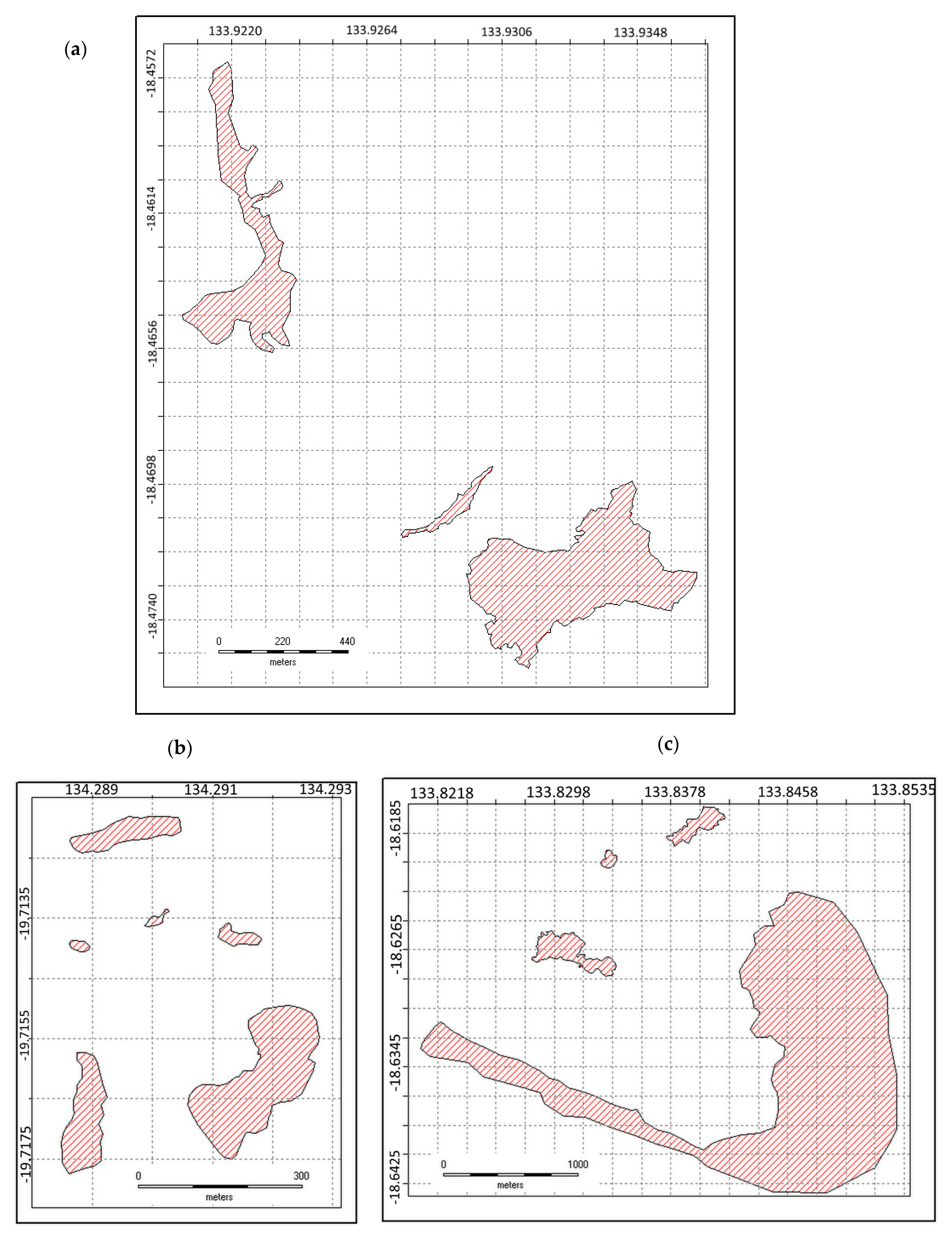
2.1. Study Sites and Species

Seed dispersal was investigated at three sites in the Barkly Region that differed in topography. Helen Springs (HS) (18°27′45.7″ S 133°55′19.8″ E) and Muckaty (MU) (18°37′42.5″ S 133°50′34.0″ E) are flat Mitchell grasslands used for beef cattle production that were invaded by rubber bush in the 1990s. Tennant Creek (TC) (19°43′01.2036″ S 134°17′29.3604″ E) is a hilly disused mine site that has well-established but clumped populations of rubber bush coexisting with spinifex (Triodia sp.) and native shrubs (i.e., Acacia saligna) used in revegetation (Figure 1ii). Thirty-year wind statistics were obtained from Elliott (nearest to HS and MU) and Tennant Creek weather stations. The mean long-term wind speeds and directions at 1500 h at Elliott and Tennant Creek are provided in supplementary (Figures S1 and S2).

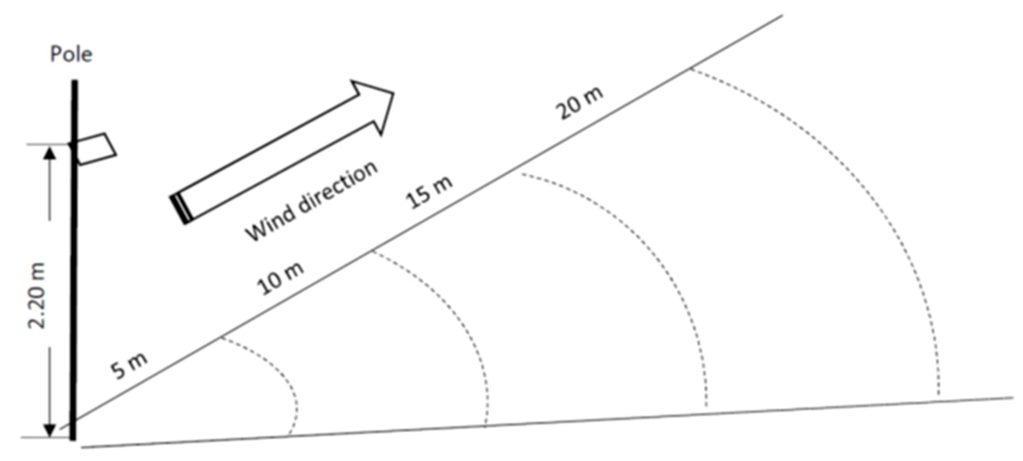
2.2. Estimating Seed Dispersal Distance

To estimate the near-distance seed dispersal kernel under natural wind conditions in the field, careful tallies were kept of all seeds that were abscised during four ten-minute intervals at each site (total 120 min) and the number of seeds dispersed into each dispersal distance bin. The number of seeds dispersed differed among simulations as seeds abscised stochastically from a fruit depending on the wind conditions. The height of the seed source was kept constant at 2.2 m. Counted seeds were sprayed with a dye.

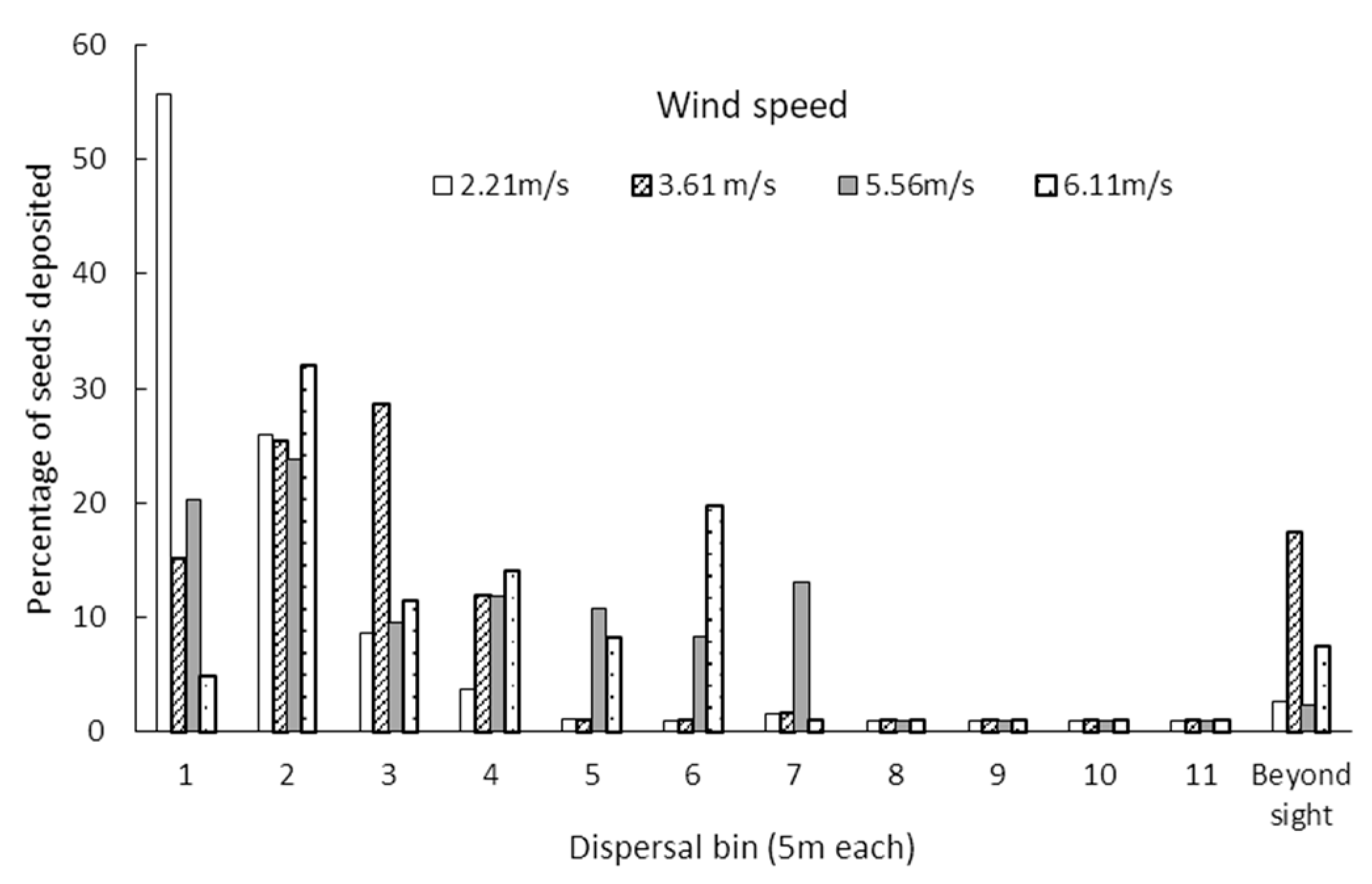
2.3. Short Distance Seed Dispersal

A challenge for this experiment was that the pappus (plume) on the seed could not be handled without causing it to collapse and thereby affect the dispersal behaviour of the seed. Hence, all mature fruit were marked and monitored until they became dehiscent and then a whole fruit was used at a time in the experiment. Six hours after dehiscence, an open fruit (Figure 1i) with plumed seeds was gently transferred onto the platform on a pole at 2.2 m high, secured using masking tape and exposed to the wind (Figure 2).

The pole height of 2.2 m reflects the mean height of rubber bush plants in the three populations [24]. All simulations were performed in the afternoon between 1400 and 1600 h to align with the Bureau of Meteorology’s long-term climatic data and to ensure seeds were sufficiently sun-dried. The pole was placed in an empty field adjacent to and downwind of a rubber bush stand. Wind speed and direction measured using a digital anemometer (Windmate 100, Instrument Choice) and compass before the commencement of each seed release. The ground around the experimental area was thoroughly inspected for any previously dispersed seeds prior to each simulation, and such seeds were sprayed with a purple dye to exclude them. Wind abscised seeds from the open fruit, blowing them onto the marked intervals on the ground and beyond (Figure 2).

After ten minutes after the start of seed release, the fruit was covered and removed. It was not possible to track each seed undergoing long-distance dispersal and ascertain its final location. However, during the 10-min seed release period, seeds were tracked when floating on the wind, and the number that floated beyond the threshold mark (55 m) was tallied and recorded first. Seeds deposited on the ground up to the threshold (i.e., eleven dispersal bins) were then counted [46]. The arc of the dispersal area was adjusted accordingly if wind direction changed during a simulation run.

2.4. Spatial Configuration of All Adjacent Populations

The edges of all contiguous rubber bush populations at the three sites were manually mapped using a Garmin GPSmap 78sc unit (Garmin International, Olathe, KA, USA). The sizes and shapes of the populations were graphically displayed in raster format with grid cells of 110 × 110 m using DIVA-GIS software [47]. The contiguous populations fitted into grids comprising 304, 35, and 221 cells for HS, TC, and MU, respectively. The proportional area of each grid cell occupied by rubber bush was determined by creating a polygon matching the shape(s) of the population(s) in a grid and calculating the proportion of the grid cell occupied using the ‘point to polygon’ routine in DIVA-GIS software [47]. These proportions were then recorded as properties of the specific grid cells and their coordinates. The data were subsequently used to characterise the spatial structure of the populations.

2.5. Modelling the Seed Dispersal Kernel

The kernel for short-distance seed dispersal can be determined under field conditions by directly counting seeds deposited on the ground within distance intervals [9,46,48]. Additionally, because of the conspicuousness of the seed pappus, rubber bush seeds floating away on the wind can be counted and included in the long-distance dispersal class even if the exact final dispersal distance remains unknown. Dispersed seeds can then potentially be partitioned into near- and long-distance dispersal categories [49,50]. If a random number of seeds abscise within a period, the proportion of those seeds deposited within a given dispersal distance interval (bin) is a random proportion of the remaining number of seeds from the previous bin. Wind seed dispersal data can therefore be modelled using any of several distribution functions that describe datasets which obey the law of proportionate effects, that is, “a process of change in which the change in the variate at any step of the process is a random proportion of the previous value of the variate” [3,51,52]. Hence, the following distributions were compared to fit the seed dispersal data:

(1)

Birnbaum–Saunders function

$$f(x ;\alpha ,\beta ) = \varphi \left(\frac{1}{\alpha }\left[{\left(\frac{x}{\beta }\right)}^{\frac{1}{2}}-{\left(\frac{\beta }{x}\right)}^{\frac{1}{2}}\right]\right)$$

where ϕ is the cumulative distribution function, α is the shape parameter, β is the location parameter or median, and x is the dispersal distance of a seed [53]. Birnbaum–Saunders is a common function utilised in survival analysis and is implemented in the Statgraphics software [54].

(2)

2-parameter exponential function

$$f(x ;\mu , \sigma )=\left(\frac{1}{\sigma }\right)exp\left\{-\frac{x-\mu }{\sigma }\right\}$$

where the threshold parameter is µ < x, the scale parameter is $\sigma >0$, and x is the dispersal distance of a seed [54].

(3)

3-parameter log logistic probability density function

$$f(x ;\alpha ,\beta ) = \frac{\frac{\beta }{\alpha }\times {\left(\frac{x}{\alpha }\right)}^{\beta -1}}{{\left(1+{\left(\frac{x}{\alpha }\right)}^{\beta }\right)}^2}$$

where α is the scale parameter, β is the shape parameter (or median), and x the dispersal distance of a seed [55].

(4)

The 3-parameter Weibull probability density function

$$f(x) = \left(\frac{\alpha }{\beta }\right){\left[\frac{x-\gamma }{\beta }\right]}^{\alpha -1}\times {\mathit{exp}}^{\left\{-{\left[\frac{x-\gamma }{\beta }\right]}^{\alpha }\right\}}$$

where α > 0 is the shape parameter, β > 0 is the scale parameter, $\mathsf{\gamma }$ is the location or shift parameter, and x is the dispersal distance of the seed [56]. In the special case where the shape is known beforehand, the only parameter requiring estimation is the scale parameter β, and the equation becomes the standard one-parameter Weibull distribution.

Satellite populations can establish at suitable downwind microsites even if long-distance dispersal occurs with low probability, provided sustained propagule pressure occurs over several fruiting seasons [15,49]. Accordingly, combining demographic and empirical seed dispersal data can potentially help reconstruct past seed dispersal events [57,58] through the evaluation of spatial and stem size patterns of plant populations [59,60] and field seed dispersal distances. In addition, combining spatial analysis of the distribution of core and satellite populations with seed dispersal allows approximation of the potential rates of movement of the invasion front through long-distance seed dispersal [57,58,59,60].

2.6. Estimation of Population Characteristics

Population growth in rubber bush can be modelled using density-dependent lagged logistic models [36]. Density-dependent logistic models are useful for representing population growth that is subject to negative feedback through reduced reproductive performance or increased mortality as the population approaches carrying capacity [61]. A suitable function is a continuous time logistic equation [62] but with a term for time lag [36]:

$$\frac{\mathrm{dN}}{\mathrm{dt}}=\mathrm{r} \mathrm{Nt}\left[1-\frac{\mathrm{N}\left(\mathrm{t}-\mathsf{\tau }\right)}{\mathrm{K}}\right]$$

where ‘r’ is the intrinsic rate of growth, and Nt is the population at time t so that the delayed effect is represented by measuring the population sizes at the time (t − τ) instead of t, where τ is the lag period. This equation does not have a definite integral because the lag time is undefined; therefore, the changes in population size are summed at various instants. Growing populations attain and surpass the carrying capacity before the feedback cycle takes effect, causing populations to follow damped oscillations under certain conditions. This form of the equation was implemented in the lagged logistic model option of the simulation program ‘Populus’ [63] that was used here.

To characterise the recruitment dynamics within the study populations, stem size frequencies were surveyed [64]. Stem circumferences above the root collars of all plants along transects that were 80 m long by 5 m wide were recorded. A total of 17 transects were assessed (six at MU, four at TC, and seven at HS), and transects were separated by 10 m and oriented from larger stemmed to smaller stemmed plants. To simplify the analysis, stem sizes at the root collar were classified as ≤10 cm, 11–20 cm, 21–50 cm, 50–100 cm, and >101 cm. Stem size was taken as an indicator of relative plant age. Static population structure in plant populations can provide important insights into plant stages that contribute to population persistence and reproductive performance [65,66], both of which are important for invasive species management. Menge and Greenfield [24] demonstrated that reproduction in rubber bush is subject to density-dependence when the population density surpasses 350–550 reproductive plants ha⁻¹, so the carrying capacity at the study locations was set at 550 reproductive plants ha⁻¹.

We used kriging to generate the best linear unbiased estimates of probabilities of infestation at all grid cells for each site. Three parameters were important in this analysis, the sill, range and nugget. The sill is the semivariance value at which the model levels off, indicating that population variations can no longer be associated with one another. The range is the distance from the origin at which the semivariance flattens out (i.e., sill occurs) [54]. In this case, we interpret the range to be the point at which the influence of a neighbouring population through seed dispersal ends. The nugget is the variance at the origin, where the semivariogram approaches the y-axis. The nugget can be viewed as the semivariance close to the source plants, in this case, with greater uniformity in population characteristics due to proximity. Semivariogram models may be used if the assumption that the data set comes from a random process with a constant mean and a spatial covariance structure that is only dependent on distance and direction between a pair of locations [67]. Three commonly used kriging models, namely, the exponential, circular and power, were fit to the dataset from each study site to examine the extent of spatial dependency and assess suitability. The three models fit to each of the datasets are [54]:

• Exponential model

$$f\left(h\right)=C_0+C\left(1-exp\left(-\frac{3h}{a}\right)\right)$$

(1)

where h = lag distance, a = range, $C_0$ = nugget variance, and $C_0+C$= sill

• Circular model

$$f\left(h\right)=C_0+C\left(1-\frac{2}{\pi }Co{s}^{-1}\left(\frac{h}{a}\right)+\frac{2h}{\pi a}\sqrt{1-\frac{h^2}{a^2}}\right) for \left\{\begin{array}{c}h\le a\\ h>a\end{array}\right\}$$

(2)

where h = lag distance, a = range, $C_0$ = nugget variance, and $C_0+C$= sill

• Power model

$$f\left(h\right)=(C_0+C)\times h^{\omega } , \mathit{for} 0<\omega <2$$

(3)

where h = lag distance, C₀ + C = sill, and $\omega$ is the power

2.7. Analyses

The effect of wind speed on rates of seed abscission was evaluated by comparing the number of seeds abscised during 10-min intervals at different wind speeds. Seed dispersal data were fitted to five probability distributions, namely Birnbaum–Saunders, exponential (2-parameter), log-logistic (3-parameter), standard Weibull, and Weibull (3-parameter) using the Statgraphics Centurion XVII software [54]. The site was included as a fixed effect in this model because of collinearity with wind speeds (in this experiment, wind speeds became a site characteristic).

Spatial autocorrelation occurs when locations close to one another show more similarity in the measured variable than those farther apart [68]. Exploration of spatial data involves computing a variogram to reveal if there is spatial dependency and to identify if there is directional bias in spread (anisotropy) [69,70]. Anisotropy is defined as the unequal spread of infestations of rubber bushes in different directions (as opposed to circular spread or isotropy). The area of a grid cell occupied by rubber bush was expressed as a proportion of the total area of the grid cell (i.e., area of infestation in a grid/area of the grid). This proportion was recorded as an attribute of the centroid coordinates of each grid cell with the grid origin at the bottom left grid cell. The two-dimensional matrices of grid positions (i.e., latitude—x and longitude—y) and the corresponding proportions of the grid cells occupied by rubber bush were analysed using kriging procedures in the Statgraphics Centurion XVII [54] software. Based on long-term prevailing wind directions (Figures S1 and S2), three compass directions (NE 45°, E 90°, and SE 135°) were examined for a spatial dependency of rubber bush population distribution. These bearings provided contrasting measures of spatial structure in wind-aligned (90° and 135°) versus a non-wind-aligned direction (45°; Figure S2).

3. Results

3.1. Seed Dispersal Kernels

To establish the threshold for long-distance dispersal, we conducted a pilot study on six transects at a typical infestation (MU) extending from the last reproductive plant into the area ahead of the invasion front.

The farthest seedling was located ~50 m from the nearest reproductive plant. We created 17 transects, each having 11 quadrats at intervals of 5 m downwind from the canopies of reproductive plants beyond the edge of the infestation, making a total distance of 55 m. The mean frequencies of plants in quadrats along transects are shown in Figure 3. There was no significant difference in the distribution patterns of plant stem sizes in quadrats between transects (F_{10, 395} = 1.54; p = 0.12), and no seedlings were located beyond 55 m. Therefore, this distance was set as the threshold for short-distance dispersal in subsequent work. There was a significant relationship (F_{1, 81} = 29.3, p < 0.0001) between stem circumference and the number of plants per quadrat as transects approached the stand edge, confirming that this was the invasion front.

On average, 96.85 ± 1.74 seeds landed within 55 m of the parent plant (i.e., 92.81%), while 7.5 ± 3.52 seeds (or 7.19%) floated beyond the threshold, demonstrating that most of the seeds attained dispersal distances that contribute to infill while a minority attained long-distance dispersal (LDD) (

Table 1. Mean ± SE of number of seeds by distance interval (bin, (m)) when all seed dispersal data were pooled (n = 143).

Distance (m)	Mean Number of Seeds	SE	Percentage
5	23.95	4.13	22.95
10	26.79	6.48	25.67
15	14.55	1.33	13.94
20	10.43	1.75	10.00
25	5.27	1.03	5.05
30	7.52	3.11	7.20
35	4.34	0.26	4.16
40	1	0.21	0.96
45	1	0.24	0.96
50	1	0.39	0.96
55	1	0.94	0.96
Beyond 55 m	7.5	3.52.	7.19

).

This minority that achieved LDD can be viewed as quite consequential for range expansion. The percentage of rubber bush seeds reaching a given distance interval (bin) appeared to be influenced by wind speed (Figure 4). However, surprisingly, the number of seeds dispersed beyond sight was highest at a medium wind speed of 3.61 m/s, particularly when updrafts peaked in hot weather.

In this analysis, we sought to compute the tail areas and critical values for the best-fitting model to evaluate seed dispersal and spread patterns. The 3-parameter Weibull model was adopted as it was both efficient (i.e., high p-value = 0.9992) and easy to implement (

Table 2. Parameters of the distribution functions fit the seed dispersal distance data with respective Kolgomorov–Smirnov test statistics (D). Higher D p-values indicate a better fit.

	Birnbaum-Saunders	Exponential (2-Parameter)	Loglogistic (3-Parameter)	Weibull	Weibull (3-Parameter)
	shape = 0.977	scale = 0.04	median = 384.055	shape = 1.683	shape = 2.175
	scale = 18.132		shape = 0.025	scale = 30.568	scale = 36.546
		lower threshold = 2.5	lower threshold = −356.699		lower threshold = −4.829
Dp-value	0.6395	0.8363	0.9998	0.9956	0.9992

). The results showed that at all wind speeds, short-distance seed dispersal is best described by a unimodal hump-shaped distribution.

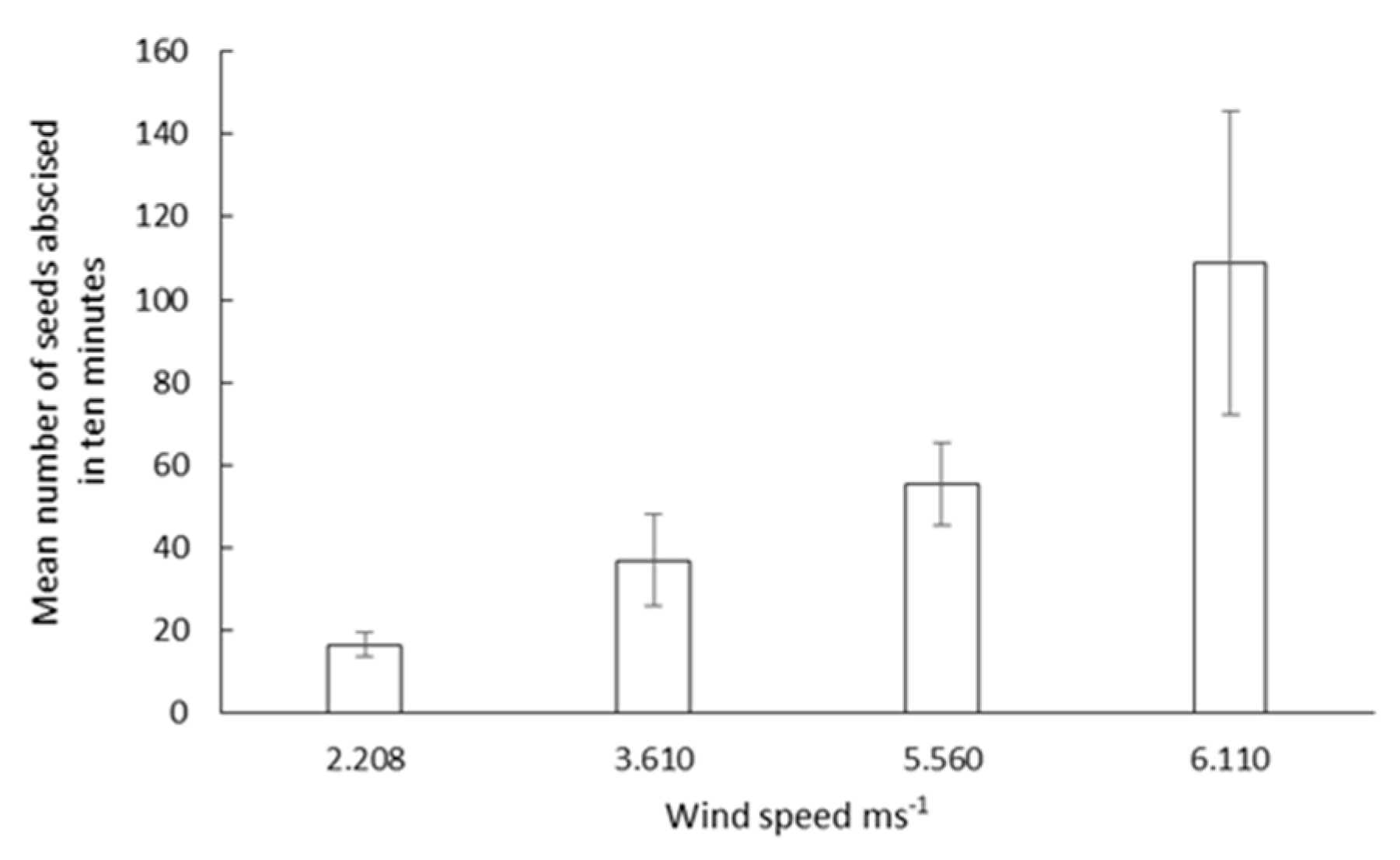
3.2. Seed Abscission

The expectation that higher rates of abscission lead to greater probabilities of long-distance dispersal was unsupported (Figure 5), even though faster wind speeds resulted in higher rates of seed abscission (Figure 6). Ultimately, the proportion of seeds that attained the high heights necessary for LDD was greatest at the relatively slow wind speed of 3.61 m/s in very warm weather typical of the Barkly Tableland.

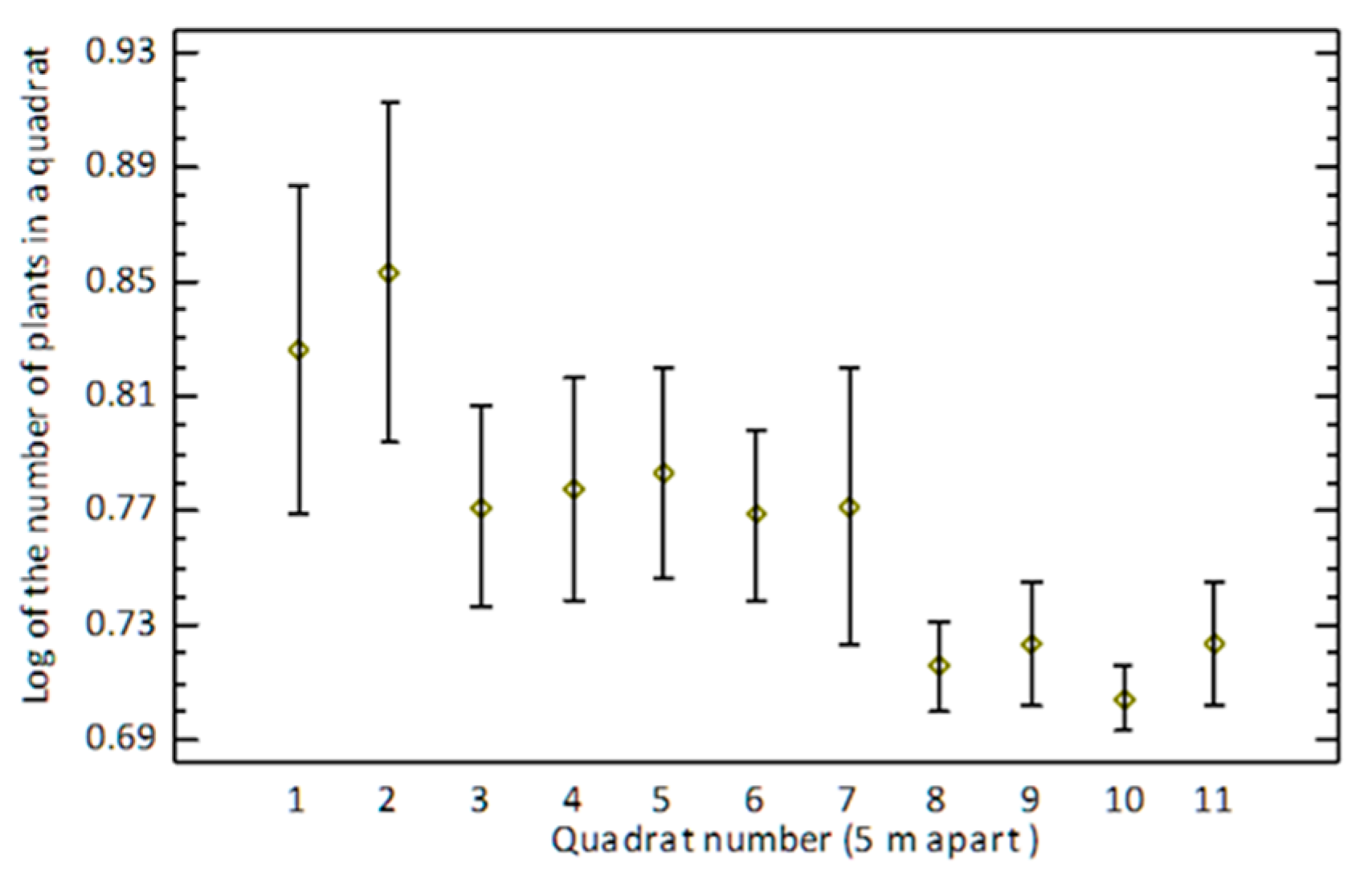
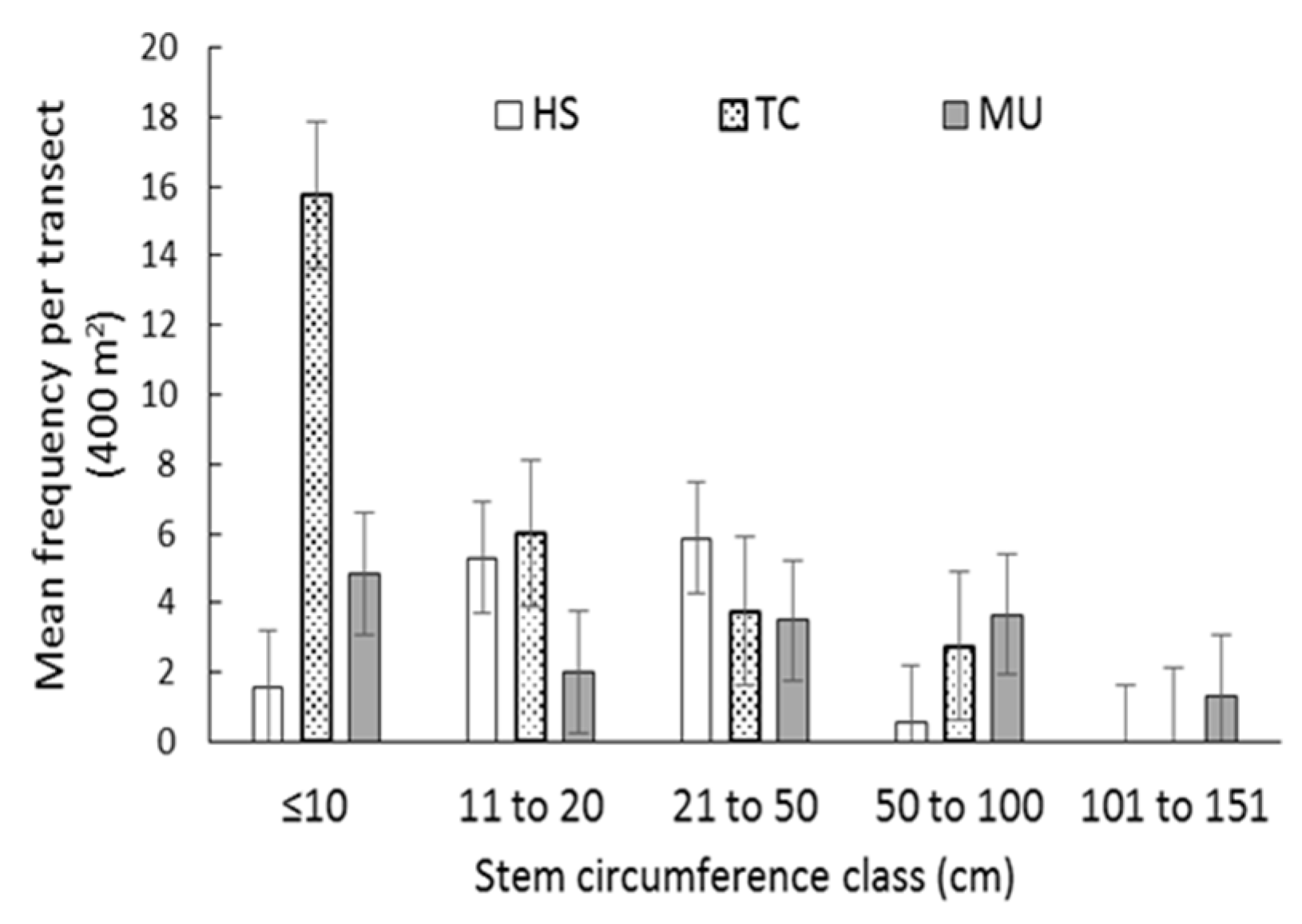
3.3. Stem Size and Spatial Characteristics of Existing Populations

Static life tables infer the historical growth of existing populations based on the assumption that age or size class mortalities remain constant over the years. In this study, the plants with the largest stems were considered to be maternal, and their locations relative to satellite populations were noted and examined further in a spatial study. MU and TC had more individuals in the seedling class, while HS had fewer seedlings but more plants in the 21–50 cm stem circumference class. The stem circumference distributions implied that HS and MU are older populations with relatively few new recruits compared to TC (Figure 7). The stem size distribution of plants also showed that a large proportion of the seedlings are established within the core population; thus, infilling is an active component of the growth of populations. Plants become reproductive when they attain stem circumferences of about 20 cm. The purpose of the analysis represented here is to determine whether each population had sufficient adult reproductive individuals to act as a source population for invasion by rubber bush. Among the three populations, MU had the oldest plants, followed by TC, while HS was relatively young. Whereas MU is likely a senescing population, TC is vigorously dispersing and invasive, while HS is a young population with considerable invasive potential unless controlled quickly. A pattern was evident: large-stemmed plants were mostly located to the southeast of the invasion front.

The spatial distribution of each population was tested for spatial autocorrelation in three directions (45°, 90°, and 135°), including two that aligned most with the long-term wind directions during the dispersal season (i.e., 90° and 135°). Directional bias was evident at MU and HS, but in both cases, less so in the 45° direction (Figure 8). This effect was less pronounced at the TC site. In all instances, seeds were assumed to be dispersed from grid cells that are on the windward side and had larger stemmed reproductive plants and deposited in cells downwind with a probability bounded by the dispersal kernel.

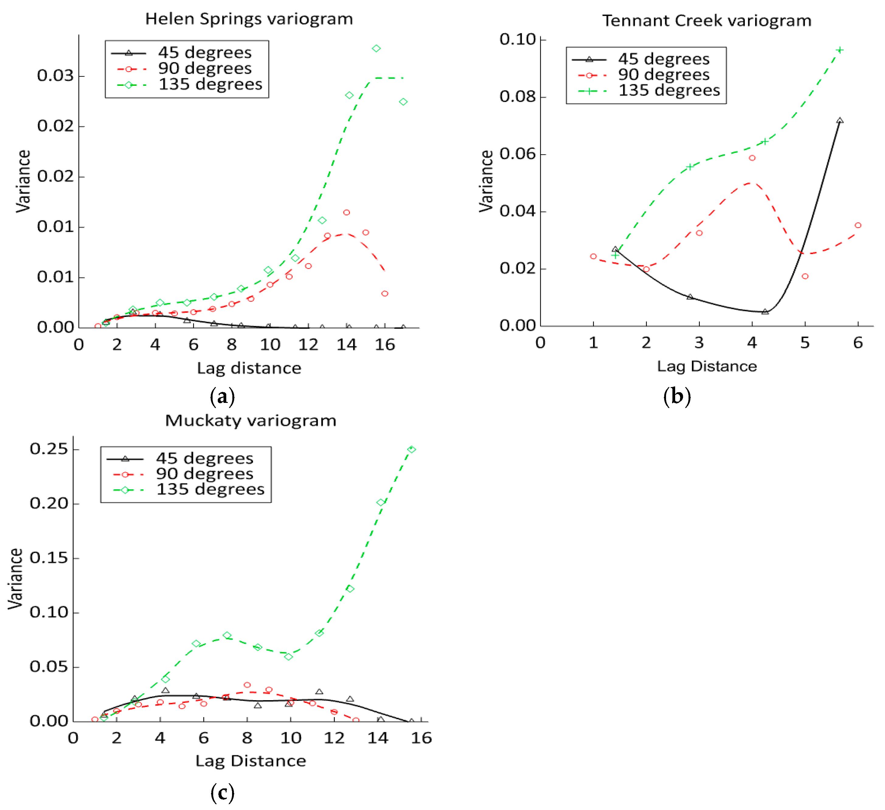
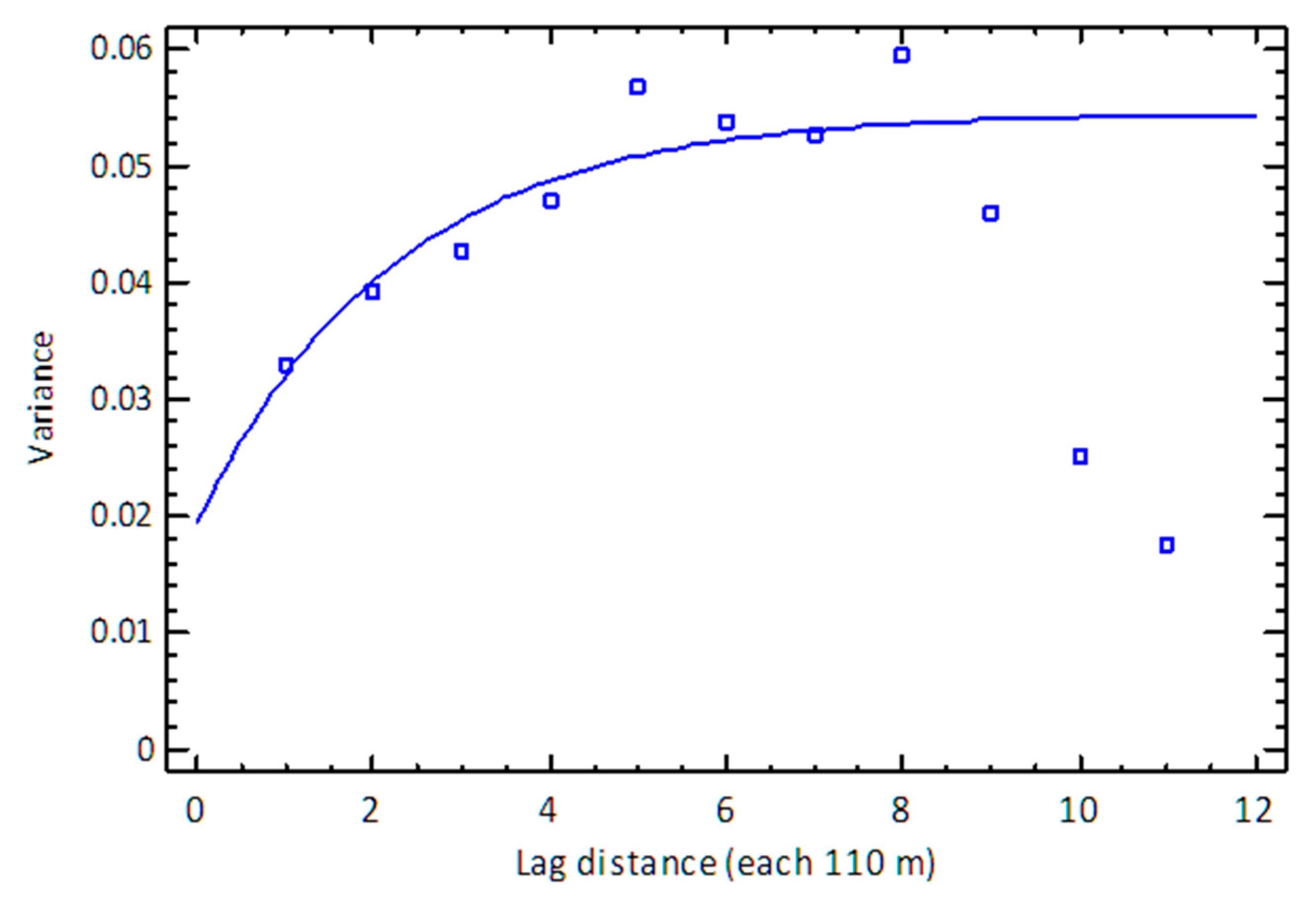
3.4. Kriging Variogram Models—The Spatial Likelihood of Invasion

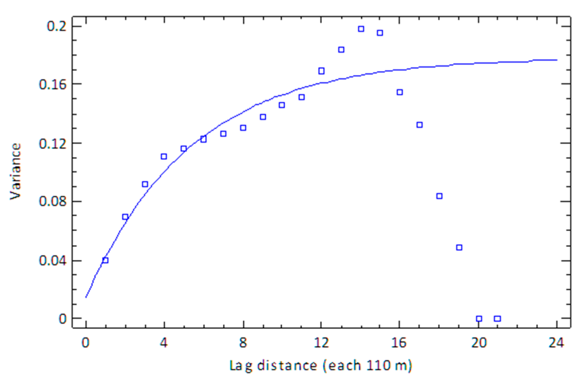
3.4.1. Tennant Creek

The proportions of cells infested with rubber bush ranged from 0.0 to 0.84, with the infestation covering a total of 42 ha. The invasion front varied in depth from 110 to 770 m along the longitude. Along the latitude, the invasion front varied in depth from 110.0 to 550 m (

Table 3. Tennant Creek sample and exponential model semivariances.

Lag (m)	Sample Semivariance	Pairs	Model Semivariance	Residual
110	0.0385	106	0.0385	0.000007
220	0.0464	122	0.0465	−0.000069
330	0.0459	120	0.0468	−0.000808
440	0.0499	146	0.0468	0.003089
550	0.0443	58	0.0468	−0.002459
660	0.0442	37	0.0468	−0.002620
770	0.0289	6	0.0468	−0.017926

). The semivariogram (Figure 9) shows the distance at which the semivariance flattens, suggesting that this is the extent of autocorrelation. The exponential model provided the best fit. Therefore, the rest were discarded.

• Exponential model

The exponential model returned a variance at the origin (nugget) = 0.039, sill = 0.047, and range = 100.8 m with R² = 63.8%. Ecologically, this means that the source population exhibited a range expansion effect over the distance of 550 to 770 m downwind.

3.4.2. Helen Springs

For Helen Springs, the proportion of a cell infested ranged from 0.0 to 0.98, and the observations covered an area of 1100 m by 880 m (or 96.8 ha). The number of observations was 80, the minimum distance between observations was 110 m, and the maximum was 1254.2 m. The mean distance between the nearest neighbours was 110 m (

Table 4. Helen Springs sample and exponential model semivariance.

Lag Distance (m)	Sample Semivariance	Pairs	Model Semivariance	Residual
110	0.0330649	268	0.0320777	0.000987
220	0.0391773	344	0.0401866	−0.001009
330	0.0427363	390	0.0453718	−0.002636
440	0.0469197	614	0.0486874	−0.001767
550	0.0568217	418	0.0508075	0.006014
660	0.0538615	440	0.0521632	0.001698
770	0.0527017	300	0.0530301	−0.000328
880	0.0594065	208	0.0535845	0.005822
990	0.0460136	140	0.0539389	−0.007925
1100	0.0251	28	0.0541656	−0.029066
1210	0.01747	10	0.0543105	−0.036841

).

• Exponential model

For HS (Figure 10), the exponential model returned a variance at the origin (nugget) = 0.039, sill = 0.047, and range = 100.8 m with R² = 63.8%. The source population exhibited a range expansion effect over a distance of 880–1100 m downwind. The fitted exponential model had a nugget = 0.033, sill = 0.055, and range = 738 m (R-squared = 70.32%).

3.4.3. Muckaty

At the MU site, the proportions of cells infested with rubber bush ranged from 0.0 to 1.0, and the longitude lag distances (x) ranged from 110 to 1540 m. Latitude (y) lag distances ranged from 110.0 to 1870 m to make a total area of 288 ha. The number of observations was 238, and the minimum distance between observations was 110 m, maximum distance of 2268.2 m. The average distance between the nearest neighbours was 110 m (

Table 5. Muckaty sample and exponential model semivariance.

Lag Distance (m)	Sample Semivariance	Pairs	Model Semivariance	Residual
110.0	0.0398248	861	0.0423905	−0.002566
220.0	0.0698433	1188	0.0654273	0.0044166
330.0	0.092287	1459	0.0845653	0.007722
440.0	0.110667	2596	0.100465	0.010203
550.0	0.1163	2045	0.113673	0.002627
660.0	0.122065	2586	0.124646	−0.002581
770.0	0.126083	2303	0.133762	−0.007679
880.0	0.130734	2414	0.141335	−0.010601
990.0	0.137636	2893	0.147627	−0.009991
1100	0.145606	2000	0.152854	−0.007247
1210	0.151494	2107	0.157196	−0.005701
1320	0.169245	1586	0.160803	0.008442
1430	0.184004	1541	0.1638	0.020204
1540	0.198532	1042	0.16629	0.032243
1650	0.195169	648	0.168358	0.026811
1760	0.155208	552	0.170076	−0.014869
1870	0.132717	230	0.171504	−0.038786
1980	0.0833853	102	0.17269	−0.089304
2090	0.0484263	40	0.173675	−0.125248
2200	0.0000250625	8	0.174493	−0.174468
2310	0.0	2	0.175173	−0.175173

).

• Exponential model

The fitted exponential model (Figure 11) had a nugget = 0.0147, sill = 0.179, range = 1780 m, and R² = 93.68%.

Kriging is used to develop models that can predict unknown values or outputs in a given location with known probabilities based on known characteristics of proximal locations. Of three models fitted for each site, the exponential model provided reasonable fits for the datasets. For HS and MU sites, the circular model proved highly unsuitable. Whereas the foregoing results demonstrated that the spatial distributions of infestations differ substantially between the flat grassland sites (i.e., HS and MU) and TC, the exponential functions can be used to model a number of aspects effectively. For example, they can be used to extrapolate the maximum distances and probabilities that new satellite populations will establish, provided the locations of mature reproductive infestations and wind characteristics are known. These models also provide an indirect approach to estimating dispersal distances in locations with similar biophysical characteristics.

3.4.4. Density Dependent Lagged Logistic Population Growth

After dispersal, seeds need favourable conditions to germinate. Bebawi and Campbell [41] reported that rubber bush plants take up to 2 years to attain reproductive maturity. It is only at this stage that local saturation and further range expansion can be feasible at the new invasion front. As shown in Figure 12 We take the 7.5% of seeds dispersed beyond the threshold of 55 m as representative of long-distance dispersal for populations with a mean plant height of 2.2 m. The proportion of the land surface in the seed shadow that is disturbed and hence suitable for colonisation should be physically estimated. The seeds have an overall germinability of 82% [19], and the fecundity is maximised at a density of 550 plants ha⁻¹ [24]. Under favourable conditions, the potential number of seedlings across the microsites under the long-distance seed shadow can be estimated as:

(a)

Seed shadow = fecundity × dispersal kernel [71];

(b)

Seedlings = Seed shadow × Ψ × 0.82

where Ψ is the assessed severity of disturbance on a scale of 0 to 1, (zero is not disturbed and one is highly disturbed bare soil) and the fecundity can be estimated from the density and size of the source population [24].

Based on the kriging ranges derived above, we conclude that satellite populations may appear at maximum distances of around 236 m at locations that have similar biophysical characteristics as the TC site and between 738 and 1780 m downwind at grassland locations that are similar to HS and MU. However, it should be remembered that these estimates are also subject to several other factors, such as edaphic and climatic conditions besides wind. Edaphic and climatic conditions affect the rate at which plants mature and reproduce, thus influencing population growth. Whereas a stage-structured matrix approach was considered, vital parameters such as survival rates are not available. We, therefore, used scenario models in Populus [63] to explore the potential effects of realistic environmental conditions on the trajectories of rubber bush populations.

Scenario 1.

Density dependent growth under favourable conditions.

In this scenario, all conditions are suitable, and a population is only constrained by the carrying capacity. We adopted 550 reproductive plants ha⁻¹ as the carrying capacity [24] with an initial population size of 5 plants and modelled population growth at 3 intrinsic growth rates (0.2, 0.5, and 0.75). Under density-dependent lagged logistic growth, the population trajectories become increasingly unstable with an increasing intrinsic growth rate. Population growth was smooth at r = 0.2, attaining the carrying capacity in 35 years. However, when the intrinsic growth rate was set to 0.5, population growth became a damped oscillation and stabilised after 35 years, although carrying capacity was reached after approximately 10 years. When r = 0.75, the population size was in perpetual oscillation (Figure 13), which was not consistent with the observed biology of this weed. An intrinsic growth rate r = 0.2 produced a biologically congruent population trajectory and was adopted for various scenarios.

Scenario 2.

A run of years of drought causes a contraction of carrying capacity.

With a previously stable population at a carrying capacity of 550 plants ha⁻¹, prolonged drought conditions of 5–10 years cause a contraction of the carrying capacity from 550 plants ha⁻¹ to a lower density. To explore the effects of this contraction, all other factors were held constant (initial population = 550, r = 0.2, and time lag = 2) and carrying capacity set at K = 60, 120, 180, and 240 plants per hectare (Figure 14). These values were arbitrarily set below the known carrying capacity of 550 plants ha⁻¹ to evaluate the potential effects of a contraction in carrying capacity. If drought causes the carrying capacity to drop to 60 individuals ha⁻¹, the population dies back to very low densities and may be extirpated within 4–5 years of drought, consistent with field observations in both Australia [42] and Senegal [44].

Scenario 3.

A run of years of drought causes a contraction of carrying capacity and extended lag periods.

In a previously stable population at a carrying capacity of 550 plants ha−¹, prolonged drought conditions cause a contraction in the carrying capacity from K = 550 plants ha⁻¹ to K = 120 plants ha⁻¹ at r = 0.2 (which provides for stable growth). Additionally, the drought causes a lengthening of the lag period as plants take longer to reach reproductive maturity. If the lag periods are set at 3, 4, and 5 years, the population is extirpated within 7–12 years (Figure 15).

4. Findings

The present study demonstrates that: (1) the invasion of rubber bush by wind dispersal of its seeds is more pronounced on open plains where dispersal distances are maximised (738 to 1780 m) compared to areas with high vegetation or hilly topography (236 m), implying that the flat pastoral plains are more susceptible to invasion; (2) spatial distribution of existing infestations has southeast to northwest directional bias due to the prevailing southeast to northwest wind direction during the seed dispersal season; (3) satellite populations ahead of the invasion front tend to be patchy, but the main front is continuous because suitable microsites are colonised first, followed by in-filling; and (4) the spread of rubber bush is not random in the prevailing wind directions, indicating a need for management downwind of stands. For sites with similar biophysical characteristics, the exponential model may be used to approximate range expansion.

5. Discussion

We confirmed our prediction that seed abscission increases with wind speed but, the relationship between wind speed and long-distance dispersal was not clear-cut and at odds with theoretical expectations [2]. This may be due to, among other reasons, the limited range of wind speeds sampled during the field experiment and the influence of ground temperature on the convective wind. There was a strong directional dependency in the spatial data along the long-term mean wind directions during the dispersal seasons [72]. In all cases, younger plants were found intermingled with larger stemmed plants in the core populations, with satellite populations having mostly younger plants. This suggests that infilling is a significant feature of the expansion of those populations, and spatial autocorrelation is indicative of the influence of dispersal on range expansion at all experimental locations.

Clark and Poulsen [73] explored ways in which near and far seed dispersal can be modelled based on seed shadow = fecundity × dispersal kernel density. Here, we suggest that the equation can be extended so that an estimate of the number of seedlings and their approximate distribution within the dispersal kernel can be obtained as follows: Number of seedlings = (fecundity × dispersal kernel density) × germinability × the proportion of disturbed land in the seed shadow. Estimating the proportion of disturbed land and how it affects overall invasibility remains a critical gap in managing rubber bush invasibility.

Previous studies show that rubber bush seeds germinate and establish best on disturbed land [25], such as stockyards, roadsides, and bare ground with low grass density. In addition, new invasions initially tend to escape notice due to the sparse distribution of plants in the landscape [74,75]. However, once these plants attain reproductive maturity, they exert considerable propagule pressure and infilling among sparsely distributed adults occurs quickly to a threshold [24]. Management of rubber bushes in the landscape requires vigilance and the removal of immature singleton plants to avoid costly control programs that eventually become necessary. Herd sizes need to be optimised if the disturbance regime is intense and steady over time, such as during drought conditions [76]. Otherwise, a property can change from low propagule pressure and high disturbance status to a high propagule pressure-established infestation-disturbance status. At that stage, overwhelming propagule pressure can result in nearby low-disturbance locations being colonised. However, it was observed that seedlings at such locations might remain stunted for extended periods due to strong competition from native grass species [25]. Minimal invasion occurs under conditions of low disturbance and low propagule pressure, which is determined by the characteristics of the habitat invaded, wind conditions, and interventive management.

It follows that new populations formed at the invasion front are subject to a lag period of about two years while they attain reproductive maturity [41]. Additionally, environmental stress caused by, for instance, extended drought may lengthen the lag period as plants remain stunted and take longer than two years to attain the size for reproduction [41,77].

Anthropogenic disturbances such as livestock grazing or altered fire regimes are known to promote invasion by some plant species [78,79,80] However, an often underrated contributor to invasibility is the biophysical environment. For example, simulation studies by Soons, Heil [2] predicted that in grasslands, the structure of local vegetation and topographic complexity greatly influence wind dispersal distances. Soons, Heil [2] and Fort and Richards [14] also argue that long-distance wind dispersal of invasive species on flat, open grassland contributes to rapid invasion. In the current study, populations on open grassland locations (i.e., MU and HS) were more spatially autocorrelated with longer potential seed dispersal ranges compared to the hilly TC site. The possibility that topography and height of neighbouring vegetation suppressed dispersal distances achieved by rubber bush at the TC site has theoretical support [17,81,82]. Tracks used by station motor vehicles and animals to access water points were particularly susceptible to invasion (i.e., Figure 12c—a track along a fence line leading to a bore at the bottom left). A review of the historical spread of rubber bush around Northern Australia reveals that similar patterns of spread are generally applicable.

Our results and historical accounts suggest that the rate of rubber bush range expansion has been influenced by factors such as long-term rainfall patterns in addition to the frequency of long-distance seed dispersal in disturbed locations. Kowarik [83] argues that deterministic factors related to life history do not sufficiently explain the progress of biological invasions; rather, increases in populations of invading species could be due to climate change and/or induced changes in the availability and accessibility of microsites. Furthermore, a lag phase may also be an artefact of changes in sampling effort over long periods due to changes in perceptions of an invasive species [84,85,86]. In a large study encompassing tens of invasive species in Queensland, Australia [87], it was concluded that the habitat invaded played little or no role in the invasiveness of a plant species. The present study suggests otherwise. The likely explanation for the difference might be that the top determinant identified in the Queensland study was ‘invasion wave frequency’ or how often a spike in population growth was observed during a period under study. A spike in population growth could be a proxy for drought/rainfall patterns that have significant effects on the germination niches of seeds and the maturation of seedlings of invasive species such as C. procera. Dry periods are attended by a short-term build-up of seedbanks in the disturbed soils [41], while subsequent wet seasons are accompanied by mass germination and establishment characterised as an invasion wave. This can repeat over many decades. For example, rubber bush was reported in the heavily wooded tropical savannas around Katherine from the 1950s, in the Victoria River district from the 1960s and in the Northeast Kimberley (i.e., Kununurra and Wyndham) from 1965 [75]. Between 1950 and 1970, population expansion at these locations was locally vigorous but not widespread, suggesting that rubber bush may have been accidentally introduced by anthropogenic means, but its spread was restricted by the complex vegetation structure. In contrast, a population of 20 ha on the Ord River catchment, a flat area denuded of vegetation, grew to 5000 ha in five years (i.e., 1965–1969) [75] and persisted for decades afterwards, even after significant improvements in the grass cover [88]. This vigorous expansion has not been evident in the Katherine or Roper River regions where the vegetation is woody and taller, and rubber bush presence predates 1950. In the State of Queensland, rubber bush was naturalised by 1935 around Georgetown [75] and, over time, the most extensive and dense colonies were established, largely by wind dispersal, in the semiarid north in the Gulf of Carpentaria and on sandy foreshores of islands [89], mostly to the west of Georgetown.

Seed dispersal by wind gives rise to characteristic population distribution patterns because the wind is a predictable vector [81] and is laminar along prevailing directions in noncomplex topography [28,90]. Accordingly, anisotropy (i.e., biased or spatial asymmetry in population distribution) was a common feature of the study populations (Figure 12a,c). Rubber bush tended to spread northwestwards as well as westwards in this study, in the prevailing wind directions. The spatial patterns in the TC populations were slightly different compared to MU and HS, suggesting that there are different patterns of the spread of rubber bush at the location. Similarly, wind-determined patterns of spread of invasive plants have been predicted and observed in other open habitats [68,91]. A possible explanation for the differences in spatial population distribution (autocorrelation) observed between the grassland sites and TC may be that complex topography causes wind turbulence and irregular movements that disperse seeds randomly, thus obscuring otherwise clear dispersal patterns observed on open and flat terrain. In addition, the limited availability of safe sites for seedling establishment on rocky terrain at the TC site could also result in irregular range expansion. Overall, wind plays a major role in the dispersal of rubber bush seeds over distances of hundreds of metres to kilometres. Directional dispersal of rubber bush seeds indicates a higher risk of colonisation of properties downwind of existing populations; hence, location-specific weed risk and management responses are feasible. The autocorrelation of population distribution at all study sites allowed an estimate of the upper limit of long-distance dispersal to be approximately 1800 m. If we allow for a lag period of 2 years, range expansion may be around 900 m yr⁻¹. However, this remains a relatively simplistic estimate of the rate of range expansion.

There are two possible scenarios for how rubber bush has spread throughout Northern Australia. First, assuming that all rubber bush populations originated from naturalised populations near Georgetown in Queensland around 1935 [75] and that spread has been by wind dispersal, rubber bush may have spread westwards over several decades, covering a distance of >2000 km to reach Western Australia in the 1960s. However, there is no evidence of connectivity or continuity in rubber bush populations from Eastern Queensland to Western Australia. Moreover, rubber bush colonies on the Barkly Tableland are clearly recently established (the 1980s) and lie between these two extremes. A second scenario is that multiple introductions have occurred at various locations in the Northern Territory through human intervention. The source population may have been the older Georgetown population. More likely is that entirely new multiple introductions from within and without Australia occurred, associated with the movement of equipment and people during the Second World War. The latter scenario is plausible given that rubber bush seeds (including the plume) were used as stuffing material in the seats of aircraft [43,74,75] and military vehicles that travelled up and down the Stuart Highway from Darwin to Alice Springs. Additionally, the distribution of rubber bush stands in the Northern Territory appears to follow roadways, suggesting that their establishment may have been influenced by seed dispersal by vehicles and animals. Of these two scenarios, the second is more plausible, whereby humans moved rubber bush seeds long distances within Australia, a phenomenon that has been shown to occur elsewhere [92]. To understand with certainty how rubber bush has spread across Australia, more studies based on the genetic relatedness of disparate populations are recommended.

In the present study, the short-distance dispersal kernel was determined empirically, while the long-distance dispersal kernel was derived from the spatial distribution patterns of the satellite relative to core populations. This approach increases the inferential power of dispersal experiments [59] and is particularly useful when it is not feasible to follow and confirm the fates of individual propagules. Cain, Milligan [93] present an interesting review of the challenges of measuring long-distance dispersal and state that whatever the difficulties, the long-distance dispersal kernel cannot be ignored. Accordingly, in our study, both core and satellite populations were investigated concurrently with observations of seed dispersal [94,95] to obtain insights into both types of dispersal. Examined jointly with habitat invasibility (or disturbance regimes), moisture and temperature conditions [19,25], the proportion of seeds that undergo long-distance dispersal can be considered a proximate indicator of the risk of invasion of the area in the seed shadow. Even though the findings here show that the proportion of seeds that undergoes long-distance dispersal is modest (~7.5%), the weed risk posed to properties neighbouring infested ones is high because a single self-compatible plant is capable of establishing a population [24]. Additionally, during unusual weather events, the number of seeds dispersed over long distances can increase dramatically.

6. Conclusions

The present study shows that the dispersal of seeds by wind accounts for the current local and regional population distribution patterns. Increased efficiency of wind dispersal raises propagule pressure from established rubber bush populations in open grasslands. Dispersal and establishment success of rubber bush is dependent on factors such as wind conditions, vegetation height, topography, and environmental conditions, including the availability of suitable microsites. Dispersal directions and distances are pronounced on plains with short or no vegetation, compared to hilly locations or areas with tall vegetation. In designing management strategies, it should be noted that the invasion risk is higher where propagule pressure is elevated on frequently disturbed land, such as pastoral properties. Infestations on plains with short vegetation should be a priority target for rubber bush control.

References

1. Nathan, R.; Katul, G.G.; Bohrer, G.; Kuparinen, A.; Soons, M.B.; Thompson, S.E.; Trakhtenbrot, A.; Horn, H.S. Mechanistic models of seed dispersal by wind. Theor. Ecol. 2011, 4, 113–132. [Google Scholar] [CrossRef]
2. Soons, M.B.; Heil, G.W.; Nathan, R.; Katul, G. Determinants of long-distance seed dispersal by wind in grasslands. Ecology 2004, 85, 3056–3068. [Google Scholar] [CrossRef] [Green Version]
3. Bullock, J.M.; Clarke, R.T. Long distance seed dispersal by wind: Measuring and modelling the tail of the curve. Oecologia 2000, 124, 506–521. [Google Scholar] [CrossRef]
4. Moody, M.E.; Mack, R.N. Controlling the spread of plant invasions: The importance of nascent foci. J. Appl. Ecol. 1988, 25, 1009–1021. [Google Scholar] [CrossRef]
5. Kot, M.; Lewis, M.A.; van den Driesshe, P. Dispersal data and the spread of invading organisms. Ecology 1996, 77, 2027–2042. [Google Scholar] [CrossRef]
6. Neubert, M.G.; Caswell, H. Demography and dispersal: Calculation and sensitivity analysis of invasion spread for structured populations. Ecology 2000, 81, 1613–1628. [Google Scholar] [CrossRef]
7. Higgins, S.I.; Richardson, D.M. A review of models of alien plant spread. Ecol. Model. 1996, 87, 249–265. [Google Scholar] [CrossRef]
8. Satterthwaite, W.H. The importance of dispersal in determining seed versus safe site limitation of plant populations. Plant Ecol. 2007, 193, 113–130. [Google Scholar] [CrossRef]
9. Terborgh, J.; Alvarez-Loayza, P.; Dexter, K.; Cornejo, F.; Carrasco, C. Decomposing dispersal limitation: Limits on fecundity or seed distribution? J. Ecol. 2011, 99, 935–944. [Google Scholar] [CrossRef]
10. Nathan, R.; Katul, G.G.; Horn, H.S.; Thomas, S.M.; Oren, R.; Avissar, R.; Pacala, S.W.; Levin, S.A. Mechanisms of long-distance dispersal of seeds by wind. Nature 2002, 418, 409–413. [Google Scholar] [CrossRef] [PubMed]
11. Greene, D.F.; Johnson, E.A. A model of wind dispersal of winged or plumed seeds. Ecology 1989, 70, 339–347. [Google Scholar] [CrossRef]
12. Jongejans, E.; Schipper, P. Modeling seed dispersal by wind in herbacious species. Oikos 1999, 99, 362–372. [Google Scholar] [CrossRef]
13. Liu, H.; Zhang, D.; Yang, X.; Huang, Z.; Duan, S.; Wang, X. Seed dispersal and germination traits of 70 plant species inhabiting the Gurbantunggut Desert in northwest China. Sci. World J. 2014, 2014, 346405. [Google Scholar] [CrossRef] [Green Version]
14. Fort, K.P.; Richards, J.H. Does seed dispersal limit initiation of primary succession in desert playas? Am. J. Bot. 1998, 85, 1722–1731. [Google Scholar] [CrossRef] [PubMed]
15. Horn, H.S.; Nathan, R.; Kaplan, S.R. Long-distance dispersal of tree seeds by wind. Ecol. Res. 2001, 16, 877–885. [Google Scholar] [CrossRef]
16. Tackenberg, O. Modeling long-distance dispersal of plant diaspores by wind. Ecol. Monogr. 2003, 73, 173–189. [Google Scholar] [CrossRef]
17. Davies, K.W.; Sheley, R.L. Influence of neighboring vegetation height on seed dispersal: Implications for invasive plant management. Weed Sci. 2007, 55, 626–630. [Google Scholar] [CrossRef]
18. Thomson, F.J.; Moles, A.T.; Auld, T.D.; Kingsford, R.T. Seed dispersal distance is more strongly correlated with plant height than with seed mass. J. Ecol. 2011, 99, 1299–1307. [Google Scholar] [CrossRef]
19. Menge, E.O.; Bellairs, S.M.; Lawes, M.J. Seed-germination responses of Calotropis procera (Asclepiadaceae) to temperature and water stress in northern Australia. Aust. J. Bot. 2016, 64, 441–450. [Google Scholar] [CrossRef]
20. Menge, E.O.; Stobo-Wilson, A.; Oliveira, S.L.J.; Lawes, M.J. The potential distribution of the woody weed Calotropis procera (Aiton) W.T. Aiton (Asclepiadaceae) in Australia. Rangel. J. 2016, 38, 35–46. [Google Scholar] [CrossRef]
21. Vitelli, J.; Madigan, B.; Wilkinson, P.; van Haaren, P. Calotrope (Calotropis procera) control. Rangel. J 2008, 30, 339–348. [Google Scholar] [CrossRef]
22. Dhileepan, K. Prospects for the classical biological control of Calotropis procera (Apocynaceae) using co-evolved insects. Biocontrol Sci. Technol. 2014, 24, 977–998. [Google Scholar] [CrossRef]
23. Campbell, S.; Roden, L.; Crowley, C. Calotrope (Calotropis procera): A weed on the move in northern Queensland. In Proceedings of the 12th Queensland Weed Symposium, Hervey Bay, QLD, Australia, 15–18 July 2013; Weed Society of Queensland: Brisbane, QLD, Australia, 2013. [Google Scholar]
24. Menge, E.O.; Greenfield, M.L.; McConchie, C.A.; Bellairs, S.M.; Lawes, M.J. Density-dependent reproduction and pollen limitation in an invasive milkweed, Calotropis procera (Ait.) R.Br. Apocynaceae. Austral. Ecol. 2017, 42, 61–71. [Google Scholar] [CrossRef]
25. Menge, E.O.; Bellairs, S.M.; Lawes, M.J. Disturbance-dependent invasion of the woody weed, Calotropis procera, in Australian rangelands. Rangel. J. 2017, 39, 201–211. [Google Scholar] [CrossRef]
26. Menge, E.O.; McConchie, C.A.; Brown, G.; Lawes, M.J. Pollinators and mating system of Calotropis procera (Ait.) W.T. Aiton (Asclepiadaceae) in an invaded range. In Proceedings of the Ecological Society of Australia Annual Conference 2015, Hilton Hotel Adelaide, South Australia, 29 November–3 December 2015; Ecological Society of Australia: Windsor, QLD, Australia, 2015; p. 12. [Google Scholar]
27. Richardson, D.M.; Rejmánek, M. Conifers as invasive aliens: A global survey and predictive framework. Divers. Distrib. 2004, 10, 321–331. [Google Scholar] [CrossRef]
28. Finardi, S.; Morselli, M.G.; Jeannet, P.; Szepesi, D.J.; Vergeiner, I.; Deligiannis, P.; Lagouvardos, K.; Planinsek, A.; Borrel, L.; Fekete, K.; et al. Wind flow models over complex terrain for dispersion calculations. In Report of Working Group 4 Cost Action 710; Finardi, S., Morselli, M., Jeannet, P., Eds.; Aarhus University: Aarhus, Denmark, 1997. [Google Scholar]
29. Fisher, A. Biogeography and conservation of Mitchell grasslands in northern Australia. In Faculty of Science, Information Technology and Education; Northern Territory University: Darwin, Australia, 2001; p. 557. [Google Scholar]
30. Cousens, R.; Dytham, C.; Law, R. Dispersal in Plants: A Population Perspective; OUP: Oxford, UK, 2008; p. 220. [Google Scholar]
31. Greene, D.F. The role of abscission in long-distance seed dispersal by the wind. Ecology 2005, 86, 3105–3110. [Google Scholar] [CrossRef]
32. Pazos, G.E.; Greene, D.F.; Katul, G.; Bertiller, M.B.; Soons, M.B. Seed dispersal by wind: Towards a conceptual framework of seed abscission and its contribution to long-distance dispersal. J. Ecol. 2013, 101, 889–904. [Google Scholar] [CrossRef]
33. Arim, M.; Abades, S.R.; Neill, P.E.; Lima, M.; Marquet, P.A. Spread dynamics of invasive species. Proc. Natl. Acad. Sci. USA 2006, 103, 374–378. [Google Scholar] [CrossRef] [Green Version]
34. Shigesada, N.; Kawasaki, K. Biological Invasions: Theory and Practice; Oxford University Press: Oxford, UK, 1997; p. 224. [Google Scholar]
35. Hanski, I.; Foley, P.; Hassell, M. Random walks in a metapopulation: How much density dependence is necessary for long-term persistence? J. Anim. Ecol. 1996, 65, 274–282. [Google Scholar] [CrossRef]
36. Renshaw, E. Time-lag models of population growth. In Modelling Biological Populations in Space and Time; Cambridge University Press: Cambridge, UK, 1991; pp. 87–127. [Google Scholar] [CrossRef]
37. Warren, I.; Robert, J.; Ursell, T.; Keiser, A.D.; Bradford, M.A. Habitat, dispersal and propagule pressure control exotic plant infilling within an invaded range. Ecosphere 2013, 4, 1–12. [Google Scholar] [CrossRef]
38. Parker, I.M. Mating patterns and rates of biological invasion. Proc. Natl. Acad. Sci. USA 2004, 101, 13695–13696. [Google Scholar] [CrossRef] [Green Version]
39. Allee, W.C. Animal Aggregations: A Study in General Sociology; University of Chicago Press: Chicago, IL, USA, 1931. [Google Scholar]
40. Taylor, C.M.; Hastings, A. Allee effects in biological invasions. Ecol. Lett. 2005, 8, 895–908. [Google Scholar] [CrossRef]
41. Bebawi, F.F.; Campbell, S.D.; Mayer, R.J. Seed bank longevity and age to reproductive maturity of Calotropis procera (Aiton) W.T. Aiton in the dry tropics of northern Queensland. Rangel. J. 2015, 37, 239–247. [Google Scholar] [CrossRef]
42. Bastin, G.; Ludwig, J.; Eager, R.; Liedloff, A.; Andison, R.; Cobiac, M. Vegetation changes in a semiarid tropical savanna, northern Australia: 1973–2002. Rangel. J. 2003, 25, 3–19. [Google Scholar] [CrossRef]
43. Foran, B.D.; Bastin, G.; Hill, B. The pasture dynamics and management of two rangeland communities in the Victoria River District of the Northern Territory. Aust. Rangel. J. 1985, 7, 107–113. [Google Scholar] [CrossRef]
44. Vincke, C.; Diedhiou, I.; Grouzis, M. Long term dynamics and structure of woody vegetation in the Ferlo (Senegal). J. Arid Environ. 2010, 74, 268–276. [Google Scholar] [CrossRef]
45. Bullock, J.M.; Shea, K.; Skarpaas, O. Measuring plant dispersal: An introduction to field methods and experimental design. Plant Ecol. 2006, 186, 217–234. [Google Scholar] [CrossRef]
46. Willson, M.F. Dispersal mode, seed shadows, and colonization patterns. Vegetatio 1993, 107, 261–280. [Google Scholar] [CrossRef]
47. Hijmans, R.J.; Guarino, L.; Mathur, P. DIVA-GIS, Version 7.5 Manual. 2012.
48. Jongejans, E.; Telenius, A. Field experiments on seed dispersal by wind in ten umbelliferous species (Apiaceae). Plant Ecol. 2001, 152, 67–78. [Google Scholar] [CrossRef]
49. Higgins, S.I.; Richardson, D.M. Predicting plant migration rates in a changing world: The role of long-distance dispersal. Am. Nat. 1999, 153, 464–475. [Google Scholar] [CrossRef]
50. Nathan, R.; Perry, G.; Cronin, J.T.; Strand, A.E.; Cain, M.L. Methods for estimating long-distance dispersal. Oikos 2003, 103, 261–273. [Google Scholar] [CrossRef] [Green Version]
51. Chesher, A. Testing the law of proportionate effect. J. Ind. Econ. 1979, 27, 403–411. [Google Scholar] [CrossRef]
52. Schurr, F.M.; Steinitz, O.; Nathan, R. Plant fecundity and seed dispersal in spatially heterogeneous environments: Models, mechanisms and estimation. J. Ecol. 2008, 96, 628–641. [Google Scholar] [CrossRef]
53. Cordeiro, G.M.; Lemonte, A.J. The β-Birnbaum-Saunders distribution: An improved distribution for fatigue life modeling. Comput. Stat. Data Anal. 2011, 55, 1445–1461. [Google Scholar] [CrossRef]
54. StatPoint. Statgraphics Centurion XVII; Statpoint Technologies, Inc.: The Plains, VA, USA, 2017. [Google Scholar]
55. Singh, V.P. Three-parameter log-logistic distribution. In Entropy-Based Parameter Estimation in Hydrology; Singh, V.P., Ed.; Springer: Dordrecht, The Netherlands, 1998; pp. 297–311. [Google Scholar] [CrossRef]
56. Weibull, W. A statistical distribution function of wide applicability. ASME J. Appl. Mech. Trans. Am. Soc. Mech. Eng. 1951, 73, 293–297. [Google Scholar] [CrossRef]
57. Wiegand, T.; Jeltsch, F.; Hanski, I.; Grimm, V. Using pattern-oriented modeling for revealing hidden information: A key to reconciling ecological theory and application. Oikos 2003, 100, 209–222. [Google Scholar] [CrossRef] [Green Version]
58. Wiegand, T.; Kissling, W.D.; Cipriotti, P.A.; Aguiar, M.R. Extending point pattern analysis for objects of finite size and irregular shape. J. Ecol. 2006, 94, 825–837. [Google Scholar] [CrossRef]
59. McIntire, E.J.B.; Fajardo, A. Beyond description: The active and effective way to infer processes from spatial patterns. Ecology 2009, 90, 46–56. [Google Scholar] [CrossRef]
60. Fedriani, J.M.; Wiegand, T.; Delibes, M. Spatial pattern of adult trees and the mammal-generated seed rain in the Iberian pear. Ecography 2010, 33, 545–555. [Google Scholar] [CrossRef]
61. Gotelli, H. A primer of Ecology, 3rd ed.; Sinauer Associates: Sunderland, MA, USA, 2001. [Google Scholar]
62. Swannack, T.M. Growth Models. In Encyclopedia of Ecology, 2nd ed.; Fath, B., Ed.; Elsevier: Oxford, UK, 2019; pp. 388–394. [Google Scholar] [CrossRef]
63. Alstad, D.N. Populus. In Simulations of Population Biology; College of Biological Sciences, University of Minnesota: Minneapolis, USA, 2015. [Google Scholar]
64. Harsch, M.A.; Buxton, R.; Duncan, R.P.; Hulme, P.E.; Wardle, P.; Wilmshurst, J. Causes of tree line stability: Stem growth, recruitment and mortality rates over 15 years at New Zealand Nothofagus tree lines. J. Biogeogr. 2012, 39, 2061–2071. [Google Scholar] [CrossRef]
65. Booth, B.D.; Murphy, S.D.; Swanton, C.J. Invasive Plant Ecology in Natural and Agricultural Systems, 2nd ed.; CAB International: Wallingford, UK, 2010; p. 211. [Google Scholar]
66. Cousins, S.R.; Witkowski, E.T.F.; Pfab, M.F. Elucidating patterns in the population size structure and density of Aloe plicatilis, a tree aloe endemic to the Cape fynbos, South Africa. S. Afr. J. Bot. 2014, 90, 20–36. [Google Scholar] [CrossRef] [Green Version]
67. Legendre, P.; Legendre, L. Chapter 13—Spatial analysis. In Developments in Environmental Modelling; Pierre, L., Louis, L., Eds.; Elsevier: Amsterdam, The Netherlands, 2012; pp. 785–858. [Google Scholar]
68. Dormann, C.F.; McPherson, J.M.; Araújo, M.B.; Bivand, R.; Bolliger, J.; Carl, G.; Davies, R.G.; Hirzel, A.; Jetz, W.; Kissling, W.D.; et al. Methods to account for spatial autocorrelation in the analysis of species distributional data: A review. Ecography 2007, 30, 609–628. [Google Scholar] [CrossRef] [Green Version]
69. Legendre, P.; Fortin, M.J. Spatial pattern and ecological analysis. Vegetatio 1989, 80, 107–138. [Google Scholar] [CrossRef]
70. Rossi, R.E.; Mulla, D.J.; Journel, A.G.; Franz, E.H. Geostatistical tools for modeling and interpreting ecological spatial dependence. Ecol. Monogr. 1992, 62, 277–314. [Google Scholar] [CrossRef]
71. Clark, J.S.; Silman, M.; Kern, R.; Macklin, E.; HilleRisLambers, J. Seed dispersal near and far: Patterns across temperate and tropical forests. Ecology 1999, 80, 1475–1494. [Google Scholar] [CrossRef]
72. Legendre, P.; Legendre, L. Chapter 1—Complex ecological data sets. In Developments in Environmental Modelling; Pierre, L., Louis, L., Eds.; Elsevier: Amsterdam, The Netherlands, 2012; pp. 1–57. [Google Scholar]
73. Clark, C.J.; Poulsen, J.R.; Levey, D.J.; Osenberg, C.W. Are plant populations seed limited? A critique and meta-analysis of seed addition experiments. Am. Nat. 2007, 170, 128–142. [Google Scholar] [CrossRef]
74. Hall, N.H. Noxious Weeds: Rubber Bush; Pamphlet; Primary Industries Branch; no. 13: Darwin, Australia, 1967. [Google Scholar]
75. Parsons, W.T.; Cuthbertson, E.G. Noxious Weeds of Australia; CSIRO Publishing: Melbourne, Australia, 2001. [Google Scholar]
76. Accatino, F.; Ward, D.; Wiegand, K.; De Michele, C. Carrying capacity in arid rangelands during droughts: The role of temporal and spatial thresholds. Animal 2017, 11, 309–317. [Google Scholar] [CrossRef]
77. Wilbur, H.M.; Rudolf, V.H.W. Life-history evolution in uncertain environments: Bet hedging in time. Am. Nat. 2006, 168, 398–411. [Google Scholar] [CrossRef]
78. Catford, J.A.; Daehler, C.C.; Murphy, H.T.; Sheppard, A.W.; Hardesty, B.D.; Westcott, D.A.; Rejmánek, M.; Bellingham, P.J.; Pergl, J.; Horvitz, C.C.; et al. The intermediate disturbance hypothesis and plant invasions: Implications for species richness and management. Perspect. Plant Ecol. Evol. Syst. 2012, 14, 231–241. [Google Scholar] [CrossRef]
79. Chambers, J.C.; Bradley, B.A.; Brown, C.S.; D’Antonio, C.; Germino, M.J.; Grace, J.B.; Hardegree, S.P.; Miller, R.F.; Pyke, D.A. Resilience to stress and disturbance, and resistance to Bromus tectorum L. invasion in cold desert shrublands of Western North America. Ecosystems 2013, 17, 360–375. [Google Scholar] [CrossRef]
80. Hierro, J.L.; Villarreal, D.; Eren, Ö.; Graham, J.M.; Callaway, R.M. Disturbance facilitates invasion: The effects are stronger abroad than at home. Am. Nat. 2006, 168, 144–156. [Google Scholar] [CrossRef] [PubMed]
81. Sorensen, A.E. Seed dispersal and the spread of weeds. In Proceedings of the VI International Symposium on Biological Control of Weeds, Vancouver, BC, Canada, 19–25 August 1984; pp. 121–126. [Google Scholar]
82. Marushia, R.G.; Holt, J.S. The effects of habitat on dispersal patterns of an invasive thistle, Cynara Cardunculus. Biol. Invasions 2006, 8, 577–594. [Google Scholar] [CrossRef]
83. Kowarik, I. Time lags in biological invasions with regard to the success and failure of alien species. In Plant Invasions: General Aspects and Special Problem; Pyšek, P., Prach, K., Rejmánek, M., Wade, M., Eds.; SPB Academic Publishing: Amsterdam, The Netherlands, 1995. [Google Scholar]
84. Cousens, R.; Mortimer, M. Dynamics of Weed Populations; Cambridge University Press: Cambridge, UK, 1995. [Google Scholar]
85. Crooks, J.A. Lag times and exotic species: The ecology and management of biological invasions in slow-motion. Ecoscience 2005, 12, 316–329. [Google Scholar] [CrossRef]
86. Crooks, J.A.; Soulé, M.E. Lag times in population explosions of invasive species: Causes and implications. In Invasive Species and Biodiversity Management; Sandlund, O.T., Schei, P.J., Viken, A., Eds.; Kluwer Academic Press: Dordrecht, The Netherlands, 1999; pp. 103–125. [Google Scholar]
87. Osunkoya, O.O.; Lock, C.B.; Dhileepan, K.; Buru, J.C. Lag times and invasion dynamics of established and emerging weeds: Insights from herbarium records of Queensland, Australia. Biol. Invasions 2021, 23, 3383–3408. [Google Scholar] [CrossRef]
88. Payne, A.L.; Watson, I.W.; Novelly, P.E. Spectacular Recovery in the Ord River Catchment; Department of Agriculture and Food: Perth, WA, Australia, 2004; p. 47. [Google Scholar]
89. DAF. Calotrope (Calotropis procera); The Government of Queensland: Brisbane, Australia, 2016; p. 3. [Google Scholar]
90. van Putten, B.; Visser, M.D.; Muller-Landau, H.C.; Jansen, P.A. Distorted-distance models for directional dispersal: A general framework with application to a wind-dispersed tree. Methods Ecol. Evol. 2012, 3, 642–652. [Google Scholar] [CrossRef]
91. Epperson, B.K. Estimating dispersal from short distance spatial autocorrelation. Heredity 2005, 95, 7–15. [Google Scholar] [CrossRef] [Green Version]
92. Ansong, M.; Pickering, C. Are weeds hitchhiking a ride on your car? A systematic review of seed dispersal on cars. PLoS ONE 2013, 8, e80275. [Google Scholar] [CrossRef] [Green Version]
93. Cain, M.L.; Milligan, B.G.; Strand, A.E. Long-distance seed dispersal in plant populations. Am. J. Bot. 2000, 87, 1217–1227. [Google Scholar] [CrossRef] [Green Version]
94. Bass, D.A.; Crossman, N.D.; Lawrie, S.L.; Lethbridge, M.R. The importance of population growth, seed dispersal and habitat suitability in determining plant invasiveness. Euphytica 2006, 148, 97–109. [Google Scholar] [CrossRef]
95. Kolb, A.; Dahlgren, J.P.; Ehrlén, J. Population size affects vital rates but not population growth rate of a perennial plant. Ecology 2010, 91, 3210–3217. [Google Scholar] [CrossRef]
Figure 1. (i) Naturally dehisced rubber bush fruit with seeds starting to abscise. Note the delicate pappus. (ii) Physical appearances of the three study sites and their infestations.
Land 12 00549 g001
Figure 2. Seed dispersal experimental set-up. Dehisced fruit was secured at the platform on the pole. There were 11 dispersal bins at 5 m intervals, making a threshold of 55 m.
Land 12 00549 g002
Figure 3. Mean distribution (95% confidence interval) of number of plants in quadrats along six transects at the leeward edge of the Muckaty infestation. These data were used to (a) select the threshold for short-distance dispersal and (b) fit a model to the stem circumference distribution data across transects (y = (9.01 − 0.0003x2)2; F1, 82 = 29.33, p = 0.00 and R2 = 26.58). Where y is the log of number of plants, and x is the stem circumference. The invasion front was determined based on smaller stemmed plants towards the stand edge, while the size of larger stems at the stand centre yielded the stand age.
Land 12 00549 g003
Figure 4. Percentage of seeds deposited within progressive dispersal intervals at four wind speeds. At a wind speed of 3.61 m/s, a relatively large proportion of seeds achieved long-distance dispersal.
Land 12 00549 g004
Figure 5. Weibull seed dispersal probability distributions at wind speeds (a) 2.028 m/s; (b) 5.56 m/s; (c) 3.61 m/s; (d) 6.11 m/s.
Land 12 00549 g005
Figure 6. The mean (±1 SE) rates of seed abscission at different wind speeds. The rates of seed abscission increased with wind speed. However, the data show the optimal wind speed to maximize height attained by the seed; hence, long-distance dispersal is 3.61 m/s.
Land 12 00549 g006
Figure 7. Stem-circumference size distribution at three study sites. TC site had relatively more saplings compared to HS and MU, indicating that it is undergoing vigorous recruitment.
Land 12 00549 g007
Figure 8. Exploratory semivariance distribution at study sites (a) HS, (b) TC and (c) MU in three compass directions, NE, E, and SE, showing that there was pronounced spatial autocorrelation in population distribution along the 135° and, to a lesser extent, 90° compass directions at all sites. Spatial autocorrelation could not be discerned for the 45° compass direction. Autocorrelation was much more pronounced in HS and MU sites that are both flat with low vegetation.
Land 12 00549 g008
Figure 9. Tennant Creek exponential semivariogram model.
Land 12 00549 g009
Figure 10. Exponential model fit to HS data.
Land 12 00549 g010
Figure 11. The fitted exponential model for MU site.
Land 12 00549 g011
Figure 12. Rubber bush population distribution patterns: The extent and shape of infestations at (a) Helen Springs, (b) Tennant Creek, and (c) Muckaty paddock, all in the Barkly region. The populations in (a,c) above are located on flat grasslands, characteristic of the Barkly Tablelands, while (b) is located in a hilly, disused mining area. In all cases, the largest populations with larger stemmed maternal plants are located to the southeast of the extended expansion fronts.
Land 12 00549 g012
Figure 13. Population growth trajectories under the lagged logistic population growth model with a lag period τ = 2 years, initial population of 5 plants, at three intrinsic growth rates (r) 0.2, 0.5, and 0.75, and carrying capacity K = 550. The population growth curve was smooth with r = 0.2, and the carrying capacity was reached after 35 years. With r = 0.5, the population growth was a damped oscillation that stabilised only after 35 years. With r = 0.75, the population size oscillated perpetually.
Land 12 00549 g013
Figure 14. Four population growth trajectories under the density-dependent lagged logistic population growth model with a lag period τ = 2 years, intrinsic growth rate r = 0.2, initial population of 550 plants, and K = 60, 120, 180, and 240. Changes in carrying capacity cause sharp declines in the population within three years but do not cause total collapse except when K = 60 when the population declines to near zero.
Land 12 00549 g014
Figure 15. Effects of reducing carrying capacity while lengthening the lag period to 3, 4, and 5 years due to delayed maturity. The population fails within 7–12 years. The population collapse reported here resembles actual observed declines of rubber bush populations during periods of droughts [42].
Land 12 00549 g015