Article

Evaluating Differences between Ground-Based and Satellite-Derived Measurements of Urban Heat: The Role of Land Cover Classes in Portland, Oregon and Washington, D.C.

1
School of Urban Studies and Planning, Portland State University, Portland, OR 97207, USA
2
Department of Fisheries, Wildlife and Conservation Sciences, Oregon State University, Corvallis, OR 97331, USA
*
Author to whom correspondence should be addressed.
Land 2023, 12(3), 562; https://doi.org/10.3390/land12030562
Submission received: 5 December 2022 / Revised: 21 February 2023 / Accepted: 22 February 2023 / Published: 25 February 2023
(This article belongs to the Special Issue How Do Land–Climate Interactions Affect Urban Heat Islands?)

Abstract

:
The distinction between satellite-based land surface temperature (LST) and air temperature has become an increasingly important part of managing urban heat islands. While the preponderance of urban heat research relies on LST, the emergence of a growing infrastructure of publicly available consumer oriented, ground-based sensor networks has offered an alternative for characterizing microscale differences in temperatures. Recent evidence suggests large differences between LST and air temperatures, yet discerning the reason for these differences between satellite-derived measurements of urban heat islands (UHI) and ground-based measurements of air temperature remains largely unresolved. In this study, we draw on an unusually robust and spatially exhaustive dataset of air temperature in two distinct bioclimates—Portland, Oregon, USA and Washington, D.C., USA—to evaluate the role of land cover on temperature. Our findings suggest that LST in highly built environments is consistently higher than recorded air temperatures, at times varying upwards of 15-degree Celsius, while forested areas contain between 2.5 and 3.5-degree Celsius lower temperatures than LST would otherwise indicate. Furthermore, our analyses points to the effects of land use and land cover features and other geophysical processes may have in determining differences in heat measurements across the two locations. The strength of the present analyses also highlights the importance of hyperlocal scales of data used in conjunction with coarser grain satellite derived data to inform urban heat assessments. Our results suggest a consistent pattern in both study areas, which can further our capacity to develop predictive models of air temperature using freely available descriptions of LST.

1. Introduction

Extreme heat is an increasingly important aspect of living in cities. The frequency and intensity of heat waves are generating impacts on public health, infrastructure, and regional ecosystems [1,2]. The extant literature on urban heat largely describes its causes and effects, as well as methods to calculate growing temperatures and examinations of remediation techniques [2,3,4]. In these studies, a recognition of the urban heat island (UHI) effect—the phenomena in which urban areas exhibit higher temperatures when compared with surrounding semi/non-urban areas [3]—and its attribution to two landscape factors, increased urbanization and the use of human-made materials in construction and increased anthropogenic heat production [4], is apparent. There are multiple adverse effects of UHI as well, including contributions to global warming, increased urban energy demands, and increased rates of heat related mortality in populations [5]. An estimated 3 billion people are directly exposed to UHIs [3], making this a global challenge faced by populations and geographies across the planet.
Of the multiple methods available for measuring urban temperatures and UHI intensity, three common approaches are well established. The first involves calculating LST, a calculation of the radiative load of the surface of the earth, using remote imaging techniques. This relies on satellite remote sensing techniques and images, and may include descriptions of land features in calculations [6,7,8]. The most common images used to calculate LST are satellite images obtained from Landsat, Moderate Resolution Imaging Spectroradiometer (MODIS), and Advanced Spaceborne Thermal Emission and Reflection Radiometer (ASTER). While they are generally freely available, these datasets lack measurements of humidity (absolute or relative), are coarser (30 m, 90 m, 1 km, etc.), and are derived from the tops of surfaces, which arguably limits our understanding of the human experience of temperatures.
A second approach, drawing from using mesoscale networks of surface weather stations, has been established to provide measurements in urban airsheds [9,10,11,12,13,14,15]. Such networks of surface weather stations can provide neighborhood-scale measurements of temperature and humidity in a city. This approach is versatile, and is especially useful for urban areas that do not have weather stations or have sparsely placed weather stations [16,17]. Furthermore, the data obtained with mobile sensors are directly relevant to human comfort because they can measure temperature, humidity, wind speed, solar radiation, and several other relevant metrological factors over continuous periods [18,19]. Some of the challenges with mesoscale networks of air temperature stations are that they are sometimes located in open, grassy fields outside buildup areas, according to World Meteorological Organization (WMO) guidelines, and, hence, are not representative of conditions in cities. Additionally, they can be quite costly and require considerable technical expertise to establish systematically in an urban region.
Finally, mobile measurement is commonly done with sensors carried by automobiles [20,21,22,23,24,25,26,27,28,29,30,31,32,33]. Several studies have deployed sensors carried by automobiles, pedestrians or bicyclists [34,35,36,37,38]. Automobiles have the advantage of traveling long transects in a short time, compared with pedestrians. However, the heat generated by car engines and moisture from exhaust pipes can contaminate the measurements collected using this methodology [37]. An additional consideration is that automobiles travel at a relatively high speed (more than 30 km/h), and conventional sensors may not be able to capture accurate temperature and humidity variations along the road traveled due to their slow time response.
The role of land cover is also central in understanding the distribution of urban heat. In essence, different land covers (e.g., concrete, asphalt, vegetation, water, etc.) respond to the sun’s radiation (i.e., short-wave radiation) through well-established physical phenomena, including reflection, dissipation, and absorption [38]. Harder surfaces absorb the sun’s radiation, retaining it and releasing when ambient temperatures are cooler (i.e., long-wave radiation). Green spaces, such as living trees, shrubs, and grasses, absorb the sun’s radiation, using it for photosynthetic processes. Recent findings suggest that at the city scale, the distributional effects of differences in temperature are partly due to the systematic removal of green spaces from some urban neighborhoods and their subsequent replacement with asphalt and concrete [39].
These spatial differences in our ability to mitigate the acute effects of urban heat are often contingent upon our ability to pinpoint places where extreme heat and social or infrastructure vulnerability intersect. Yet, as numerous datasets of urban heat emerge, city planners, public health staff, urban foresters, and other municipal managers and resilience professionals are unable to assess the differences between the diverse array of descriptions of urban heat and make informed choices on the best option for their needs. Consider, for example, the general availability of free satellite-derived and spatially-explicit descriptions of urban heat, which are available through Google Earth Engine, Landsat 8, and other derivative products. Despite the broad availability of satellite-derived urban heat datasets, our current understanding of the differences between LST and near surface air temperatures (NSAT) remain woefully inadequate.
Together, these urban heat and UHI intensity monitoring techniques have several advantages and disadvantages, the detailing of which is beyond the breadth of this article. Yet, perhaps due to the lack of densely co-located mesoscale temperature networks in cities, dozens of studies attempt to use widely available LST and land use/land cover (LULC) to predict NSAT or NSAT in relation to LULC. Weng et al. [40], for example, examined LULC and LST patterns in Marion County, Indiana, using Landsat ETM+ imagery. Imagery was unmixed using spectral mixture analyses, and then classified into seven LULC classes, which were then correlated with pixel-based LST measurement. Results found LST to be negatively correlated with green vegetation classes, and positively correlated with classes containing impervious surfaces. Feng et al. [41] examined the spatiotemporal dynamics of surface temperature in relation to land use change in the Taihu Lake Basin. The authors found that high-density built-up areas are the warmest land surface, followed in decreasing order by low-density built-up areas, agricultural lands, forests, and water bodies. These results followed a similar trend with our results, where temperature measurements were inverse to land classes with higher vegetation cover.
Karakus [42] examined the relationship between LULC features, NDVI (Normalized Difference Vegetation Index—a measure of relative greenness) and LST in Sivas, Turkey using Landsat imagery from 1989–2015. Results found that urban areas, with higher proportions of impervious surfaces, had the highest average temperatures, followed by bare lands (including harvested areas) and agricultural lands. NDVI had an inverse relationship with LST (with a strong correlation; with R2 values between 0.95 & 0.99), where increases in LST were seen with a decrease in NDVI values. High NDVI values were generally found in forested areas, so some inference might be possible with NDVIs and the forested LC classes in our study. In another study site in Nigeria, Africa, LULC factors explained 26–64% of the total variation found in LST readings (though, interestingly, elevation was not found to have a significant effect) [43]. Lastly, Ziter et al. [44] (in a methodology similar to our own) investigated interactions between tree canopy cover and impervious surfaces using a mobile temperature measurement system in Madison, Wisconsin. Their results also confirmed that warming caused by impervious surfaces could be countered by canopy cover, particularly when tree cover covered a radius of about 60–90 m.
Still missing from these and other studies, however, is an understanding of the relationship between LST, NSAT and the role of LULC characteristics, particularly as they vary across bioclimate regions. An understanding of how LST and NSAT vary because of differences in land cover, and the extent to which other different bioclimatic conditions play a role is needed. In response to these discussions, a study was piloted to achieve the following objectives:
  • To examine distribution patterns of LST and NSAT.
  • To predict variability of temperatures by using land cover characteristics.

2. Materials and Methods
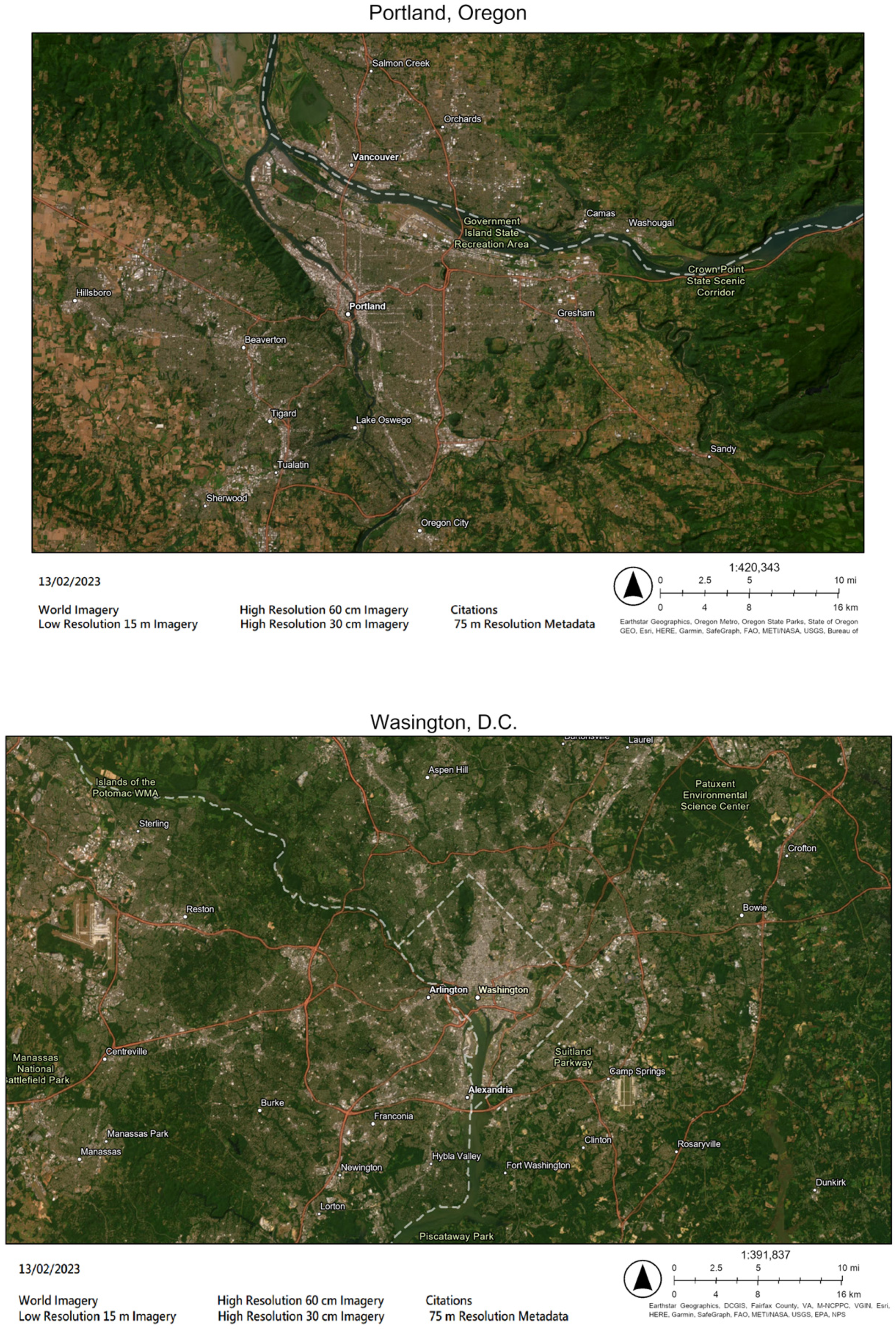
2.1. Study Area

We examined differences between LST and NSAT in Portland and Washington, D.C. metro regions, both of which represent diverse bio-climatological conditions. Washington, D.C. is located in a humid subtropical climate zone based on the Koppen Climate classification system [45]. As one of the larger metropolitan cities in the US, and as a hub for political activity, D.C. and its surrounding regions have extensive administrative buildings and a conventional street grid. Winters in the region are also trending warmer, with an increase in freeze-free season length as well as greater, more variable precipitation [46].
Similar to D.C., the Portland, Oregon area has seen increased urbanization and also contains a conventional street grid design, and is divided by two rivers. Portland has a warm-summer Mediterranean climate based on the same Koppen climate classification [45], and has seen an 11.8% increase in population since 2010 [47]. Both cities have approximately 700k inhabitants but differences exist in the predominant construction material used for housing g. Washington, D.C. residents mostly live in some form of stone housing (e.g., brick, cinderblock, brownstone, etc.), while those in Portland mostly live in wood homes [48,49]. Figure 1 (below) provides a satellite image of both the study sites.

2.2. Predicting Ambient Temperature

NSAT in Portland and Washington, D.C. was predicted using a combination of ground-based measurements, satellite imagery, and machine learning techniques, specifically Random Forest modeling [17,39,50]. For ground-based measurements, we employed vehicle-mounted temperature sensors along with a global positioning system (GPS).
This study also piloted the mass deployment of a smart sensor that satisfies the four essential functions required for mobile measurement: sensing of temperature and humidity, data-logging, time-stamping, and geolocating. The sensor has the characteristics of IoT (Internet of Things) technology: it is light-weight and low-cost, has wireless data communication ability, and can be potentially deployed in large quantities. The sensor was mounted on the passenger side window of cars, with the sensor about a meter above the roof of the car. Temperatures were collected at a one-second interval using a type “T” thermocouple and data logger at three time periods: 6–7 AM, 3–4 PM, and 7–8 PM. We only utilized two time periods: 6–7 am and 3–4 pm, because we only examined daytime temperatures for this study. For satellite data, we used the Sentinel-2 satellite constellation, provided by the European Space Agency. We used all visible and infrared bands with either 10 m or 20 m resolution, with a total of 10 bands. The acquisition dates for Sentinel-2 were determined by the following criteria: (a) cloud coverage less than 10%, (b) dates closest to the traverse day.
Based on a preliminary study also led by one of the authors [39], we computed focal buffers for each of the 10 bands with the following distances: 50 m, 100 m, 150 m, 200 m, 250 m, 300 m, 350 m, 400 m, 450 m, 500 m, 600 m, 700 m, 800 m, 900 m, and 1000 m, creating a total of 150 variables. Next, the Random Forest Model was applied to predict ambient temperature using both temperature data and variables from the Sentinel-2 data. The accuracy of the model was tested using the ‘holdout method’, which partitions the data into two mutually exclusive subsets, called a training set and a test set. For this study, we randomly selected 70% of the traverse data as the training set and the remaining 30% of the data as the test set. Table 1 shows the adjusted R2 for all four models. Across all models, we observed that more than 87.7% of the variation in observed temperature could be explained by the model variables.

2.3. Satellite Data Used for LST

LST was derived from Landsat 8 Thermal Infrared Sensor (TIRS). In this study, we used the Climate Engine Application (https://resilienceglobale.com/information/hazards-disasters/drought/31-climate-engine.html, accessed on 10 December 2018, requires account setup with email) to obtain LST. LST calculation follows the approach described in equations 20–22 in Allen et al. [51]. The acquisition dates of Landsat for both Portland and Washington, D.C. were carefully determined based on finding Landsat images that contained less than 10% cloud cover, with the data acquisition day being within +/− 1 year from the traverse date and in either June, July, August, or September. We also gathered the maximum temperature at a nearby airport using the Weather Underground website and data (https://www.wunderground.com/history/monthly/us/or/portland/KPDX/date/2018-7, accessed on 10 December 2018). Finally, we calculated the temperature difference to the traverse day, and selected the satellite image with the closest date (Table 2).
As Landsat 8 data were acquired around 10 am in the Portland region and 12 pm in Washington D.C., both local times. These times were different than the collection of NSAT and required additional revisions and interpolations to conduct timely comparisons. NSAT is also estimated at noon based on the morning (6–7 am) and afternoon (3–4 pm) NSAT. For Portland, we examined the diurnal temperature variation at a nearby airport on 29 July 2016 and on 28 August 2018 using WeatherUnderground data. For Washington, D.C., since the data on 28 August 2018 were not available, we employed both 27 August 2018 and 29 August 2018 data. Using the temperature profile for each city, the data indicated that the temperatures linearly increase from morning (6 AM) to afternoon (3 PM) in Portland, and the temperature linearly increases from morning (6 AM) to around noon (12 PM), and maintains until the afternoon (3 PM) in Washington, D.C. We employ linear interpolation for Portland and use 3 PM data as 12 PM data for Washington, D.C. Based on this approach, we conducted timely comparisons between LST and NSAT, across the two study regions.

2.4. Normalizing Temperature

Although the Landsat acquisition dates for deriving LST were carefully determined, the dates for LST and NSAT are not the same. In this study, we are interested in the spatial distributions of temperatures, but not the raw temperatures themselves; therefore, to minimize the magnitude of temperature differences on different days and reduce the range of the raw data of these temperatures, we normalized the temperatures for both LST and NSAT using Celsius (°C°C), which is consistent with other related studies. For example, in earlier studies using LST for one of the study regions (Moffett et al., 2019), the authors note several anomalies when using raw LST data for assessing heat differences. These anomalies can impact findings by skewing the surface temperatures to greater extremes.
Accordingly, the normalized temperatures are computed by subtracting the mean temperature at the study site from the raw temperatures:
Normalized LST = LST − Mean LST
Normalized NSAT = NSAT − Mean NSAT

2.5. Land Cover Data

The land cover data used for this study was taken from the National Land Cover Database [52], which were obtained from the U.S. Multi-Resolution Land Characteristics Consortium (MRLC, www.mrlc.gov, accessed on 18 January 2019). Land cover characteristics have been found to be related to temperatures, with surface temperatures higher in industrialized regions or areas with impervious surfaces, and lower in areas with vegetation or water [53,54,55]. The NLCD provides open-source data on land cover and land cover change at up to 30 m resolution. Land cover classes in the NLCD can be grouped by various categories, and the land cover classes most prevalent in the continental US, in order, are Shrub/Scrub (21.85%), Cultivated Crops (16.31), and Grasslands/Herbaceous (13.34%) [56].
Of all the classes defined, five classes (Perennial Ice/Snow, Dwarf Scrub, Sedge/Herbaceous, Lichens, and Moss) were not present in the study area and were therefore removed from our analysis. Furthermore, the Open Water class in NLCD data and cloud coverage areas in Landsat 8 data were eliminated from the following analysis. Since these land cover data have a native resolution of 30 m pixels, we resampled NSAT to the same resolution. The consistency between land cover, LST, and NSAT enable the comparison across raster images, using the 30 m as the unit of analysis.

3. Results

3.1. Descriptive Statistics

We begin by describing the descriptive statistics of LST, NSAT, LST-NSAT for each LC class at Portland and Washington, D.C (Table 3 and Table 4). For Portland, the mean temperature of normalized NSAT for each class ranges from −1.38 °C to 1.44 °C (difference = 2.82 °C), and the mean temperature of normalized LST for each class ranges from −6.04 °C to 7.63 °C (difference = 13.67 °C). For Washington, D.C., the mean temperature of NSAT for each class ranges from −1.36 °C to 0.91 °C (difference = 2.27 °C), and the mean temperature of LST for each class ranges from −3.6 °C to 2.63 °C (difference = 6.23 °C). These results suggested higher temperature variability for LST than for NSAT.
The difference between LST and NSAT (LST-NSAT Mean) indicate that LST consistently contains higher temperature measurements than NSAT at the Low-, Medium-, High- Intensity development land, and Barren Land for both study sites. LST is lower than NSAT at the other vegetated classes and Open Space class.

3.2. Spatial Distribution of Temperatures: LST & NSAT

Many of the differences between LST and NSAT are illustrated by examining the spatial distribution of the normalized temperature for each (Figure 2). The positive or negative values indicate whether the temperatures are higher or lower than the average temperatures in the study area, respectively. The maps of LST and NSAT at Portland and Washington, D.C. clearly illustrate that the spatial trends are positive; that is, higher temperatures are located around developed areas and negative, lower temperatures are located around vegetated areas.
Taken together, LST and NSAT differences also vary by region and location (Table 4). In general, the positive values indicate that LST is higher than NSAT, and negative values indicate that LST is lower than NSAT at the location. Interestingly, the positive/negative values do not seem to display a random distribution, and rather show a clear spatial pattern across both study locations (Figure 3). The regularity of spatial patterns in temperature differences supports our research question by indicating that land covers may play an important role in determining these differences.

3.3. Comparing Land Cover Attributes

When comparing the role of land cover on differences between LST and NSAT in the two study regions, we observed several consistent patterns (Figure 4). Although the magnitudes of temperatures are different in Portland and Washington, D.C., both regions reflect the same direction of temperature change (e.g., both positive as opposed to one positive difference and the other negative). Additionally, as the intensity of development increases, the difference between LST and NSAT also increases, which indicates that LST tends to be higher than NSAT as the development intensity increases. On the other hand, LST is lower than NSAT for the other vegetated areas in both study sites. LST is much lower in the forested and wetland areas compared to NSAT.
The only land cover class where Washington, D.C. has a larger difference than Portland is within the Hay/Pasture and Cultivated Crop classes. We noted that the percentages of LC for Hay/Pasture and Cultivated Crop are 0.26% and 0.55%, respectively, in Washington, D.C., and 21.48% and 4.72%, respectively, in Portland, which makes them both rare in Washington, D.C. and, hence, the results may not be representative of these classes.

3.4. Statistical Tests between LST and NSAT for Each Land Cover Class

Assessing differences between LST and NSAT for each of the land cover classes requires additional statistical tests. By comparing each land cover class and the extent to which they can help to explain differences between the two measures of urban temperatures, we can illustrate which ones might be stronger predictors of ambient temperature. The authors conducted a Paired Samples T-Test and a Pearson’s correlation coefficient to compare any correlation between land cover class and both measures of temperature (Table 5, Table 6, below). The results of the Pearson’s product-moment correlation and paired samples T-test between LST and NSAT for each class in both study regions indicate that correlations vary by class, but most classes show a strong correlation between LST and NSAT. High intensity urban development, cultivated crops, hay/pasture, and herbaceous wetland classes for the Portland region showed the weakest correlations, while Washington, D.C. had the weakest correlations, with only high intensity urban and herbaceous wetland. Among the highest correlations for both Portland and Washington, D.C. were consistencies in the forest classes. Others such as open space and low intensity urban were strong in Portland, while Washington, D.C. had other strong correlations with the barren land, shrub, and cultivated crops classes.
The T-value measures a ratio of the difference between the mean of the two sample sets and the variation that exists within the sample sets. The greater the magnitude of T, the greater the evidence against the null hypothesis, in this case the null hypothesis being no significant difference between LST and NSAT. The p-values of the T-test are all less than 0.05, and they indicated that the mean of LST and NSAT is significantly different for both study sites at a 95% confidence level.

4. Discussion

The above results allow us to compare the differences in findings between satellite derived LST and NSAT, as well as between land classes for each. Our findings provide insights for using LST and NSAT to predict temperature and determining the relationship between land cover and temperatures. Perhaps most significant of our findings is that LST and NSAT are significantly different regardless of the underlying land cover. This is significant because both measurement systems are often applied interchangeably, yet our results indicate that they are not the same, and, in fact, warrant additional assessment when being used for public policy or other decision making efforts.
Our results also corroborate previous studies’ findings regarding the spatial distribution of UHIs. Temperatures, both LST and NSAT, are noticeably higher around urbanized areas in both study sites [40,42,44,53,54,55]. The LST and NSAT measurements in land cover with impervious surfaces (i.e., developed spaces of varying levels of intensity) were higher than measurements in all other types of land covers—similar to the studies mentioned above. The differences observed in the temperatures observed between LST and NSAT may also be insightful. LST, which may not adequately capture the physical effect of temperatures on humans, may also inadequately capture the complex effect of shade on lowering temperatures—particularly building on building shade in urban areas, and tree canopy on lesser inhabited/developed areas, as discussed by Kremer et al. [57] This may explain the phenomena in which LST readings increased by a greater scale as land cover was also increasingly urbanized, in both Portland and D.C.
As mentioned above, in both study sites LST and NSAT increased as the intensity of urbanization increased and decreased in forested areas. Measurements for both in land covers with agricultural purposes (land class hay and cultivated crops) fell between these two other broad classes—possibly implying that increased vegetation/canopy size affects both measurements of temperature inversely. In all forested areas, NSAT measurements were greater than LST measurements—a surprising find, considering the effect vegetation and canopies are expected to have on heat, but suggesting that other environmental factors including rates of evaporation, transpiration and wind speeds, might also play a role in determining NSAT—some other studies, detailed below, highlight similar results. Of interest may also be the results of our paired sample t-tests—the LST and NSAT across both study sites were found to be correlated but significantly different from each other at all land classes. We might infer, hence, that land class might play a role in determining temperatures. This also corroborates findings from other studies [40,42,44,55].
As such, the importance of land uses and classes cannot be discounted when examining measurements of temperature, regardless of the methodology applied. Beyond land uses, land cover features may provide additional insight on determining LST and NSAT. For example, Larondelle et al. [58] developed a method to classify urban structure using land cover and building height and examined how urban structures in both Berlin and New York City relate to temperature. The authors found that the majority of the areas in these cities (68% in Berlin and 79% in New York City) can be represented with the same fifteen urban structure classes, and these common classes share very similar temperature patterns despite major differences in the two cities’, climate, size, and levels of built versus green space. Other recent research supports the importance of not just LULC factors, but also highlights possible inaccuracies in using only remote sensing derived temperatures. Venter et al. [59], for example, found that satellite imagery alone was ineffective in quantifying the effects evaporation has on temperatures, and, hence, LSTs were consistently overestimated—in many cases by up to six times in normalized values —when compared with temperatures calculated at the canopy level alone. Chen et al. [60] examined similar canopy heat indexes and attempted to evaluate and determine prediction methods using RS images and the Random Forrest modeling approach in Nanjing, China. They found that LULC classes had a strong effect on determining air temperatures, as did wind speed, evapotranspiration rates, and other geometric parameters (e.g., distance to city center) and relying simply on LST obtained from satellite images is insufficient to explain urban environments. In another study conducted in Dane County, Wisconsin, researchers [61] compared satellite derived LST to measurements recorded by a network of temperature sensors, and found that LST measurements displayed higher variability (results similar to ours), but particularly across agricultural and rural land (findings in contrast to our own), which the authors attributed to phenological differences across the urban and rural study sites.
While our study only examines two sites, this is still twice the number of studies conducted in previous single-case urban temperature assessments. Our study confirms the importance of land cover features, though due to a lack of relevant data is not able to comment on the importance of other environmental factors such as wind speeds, evaporation rates, and phenological or seasonal conditions. Examining NSAT gathered at finer levels may be of growing importance to capture accurate spatio-temporal heat dynamics. The development of low-cost sensors and community science programming also allows for further investigation into examining factors influencing LST and NSAT. Some applications of these sensors have been found in the use of determining urban air quality, but research conducted by Kousis et al. [62] calls for the further use of sensors capable of capturing environmental data at ultra-fine scales to adequately capture the unique scalar, vector and directionally dependent variables present within all urban environments. Several projects show promise in further integrating assessments of LST and NSAT and can potentially contribute to predicting air temperature based on remotely measured techniques.

5. Conclusions

The present paper examined the differences recorded between LST and NSAT in Portland, Oregon, and Washington, D.C., and the effect of land cover classes. Using a novel approach that integrates spatially exhaustive surface temperatures with air temperatures, we were able to illustrate that differences in land cover classes have differential effects on the two sources of urban temperatures. These differences are significant because they indicate that descriptions of LST alone can over-exaggerate the temperatures of urban areas, especially highly urbanized areas, and under-exaggerate the temperatures in forested zones. As techniques for conducting mobile monitoring become increasingly ubiquitous, methods for integrating them with satellite derived descriptions will also expand, ushering in a robust and integrated approach for measuring urban heat.
Urban heat continues to have an acute impact on urban populations, infrastructure, and ecosystems. Without striving for techniques that bring together satellite derived measurements along with mesoscale networks and mobile sensing, policy makers and planners will struggle to find the most suitable application for their needs. This study is one of the first to evaluate the differences between LST and NSAT, and future studies will need to further integrate and evaluate these differences with stationary network temperature data. Our mobile monitoring devices provided an easily deployable and accurate method of measuring, and as the field of urban climate continues to develop, we will need to use them in conjunction with satellite derived imagery and stationary networks to understanding the nuanced effects of land cover on temperature, and ultimately temperature on human health.

Author Contributions

Conceptualization: V.S. and Y.M.; Data curation: V.S. and Y.M.; Formal analysis: V.S. and Y.M.; Investigation: V.S. and Y.M.; Methodology: V.S. and Y.M.; Project administration: V.S.; Resources: V.S.; Software: V.S. and Y.M.; Supervision: V.S.; Validation: V.S., Y.M. and A.N.U.; Visualization: V.S., Y.M. and A.N.U.; Writing—original draft: V.S. and Y.M.; Writing—review & editing: V.S. and A.N.U. All authors have read and agreed to the published version of the manuscript.

Funding

This study was in part funded by the National Science Foundation (Award # 2010014), and the National Urban and Community Forestry Challenge Grant (Award #: 17-DG-11132544-014).

Data Availability Statement

The data collected for this study is publicly available on the Open Science Framework website for public access, including download. The data can be found here [www.osf.io].

Acknowledgments

The authors are indebted to the U.S. National Science Foundation, U.S. Forest Service’s National Urban and Community Forestry Challenge, and U.S. National Oceanic and Atmospheric Administration for providing different forms of support in conducting this research. The authors are also indebted to the citizen scientists who assisted in collecting air temperatures in both Portland (OR), and Washington D.C.

Conflicts of Interest

The authors declare no conflict of interest.

References

  1. Haines, A.; Kovats, R.S.; Campbell-Lendrum, D.; Corvalán, C. Climate change and human health: Impacts, vulnerability and public health. Public Health 2006, 120, 585–596. [Google Scholar] [CrossRef]
  2. Zuo, J.; Pullen, S.; Palmer, J.; Bennetts, H.; Chileshe, N.; Ma, T. Impacts of heat waves and corresponding measures: A review. J. Clean. Prod. 2015, 92, 1–12. [Google Scholar] [CrossRef]
  3. Rizwan, A.M.; Dennis, L.Y.; Chunho, L.I.U. A review on the generation, determination and mitigation of Urban Heat Island. J. Environ. Sci. 2008, 20, 120–128. [Google Scholar] [CrossRef]
  4. Mohajerani, A.; Bakaric, J.; Jeffrey-Bailey, T. The urban heat island effect, its causes, and mitigation, with reference to the thermal properties of asphalt concrete. J. Environ. Manag. 2017, 197, 522–538. [Google Scholar] [CrossRef]
  5. E.P.A. Heat Island Impacts. 2020. Available online: https://www.epa.gov/heatislands/heat-island-impacts (accessed on 2 January 2023).
  6. Peng, J.; Xie, P.; Liu, Y.; Ma, J. Urban thermal environment dynamics and associated landscape pattern factors: A case study in the Beijing metropolitan region. Remote Sens. Environ. 2016, 173, 145–155. [Google Scholar] [CrossRef]
  7. Clinton, N.; Gong, P. MODIS detected surface urban heat islands and sinks: Global locations and controls. Remote Sens. Environ. 2013, 134, 294–304. [Google Scholar] [CrossRef]
  8. Zhao, L.; Lee, X.; Smith, R.B.; Oleson, K. Strong contributions of local background climate to urban heat islands. Nature 2014, 511, 216–219. [Google Scholar] [CrossRef]
  9. Souch, C.; Grimmond, S. Applied climatology: Urban climate. Prog. Phys. Geogr. 2006, 30, 270–279. [Google Scholar] [CrossRef]
  10. Koskinen, J.T.; Poutiainen, J.; Schultz, D.M.; Joffre, S.; Koistinen, J.; Saltikoff, E.; Gregow, E.; Turtiainen, H.; Dabberdt, W.F.; Damski, J.; et al. The Helsinki Testbed: A mesoscale measurement, research, and service platform. Bull. Am. Meteorol. Soc. 2011, 92, 325–342. [Google Scholar] [CrossRef] [Green Version]
  11. Basara, J.B.; Illston, B.G.; Fiebrich, C.A.; Browder, P.D.; Morgan, C.R.; McCombs, A.; Bostic, J.P.; McPherson, R.A.; Schroeder, A.J.; Crawford, K.C. The Oklahoma city micronet. Meteorol. Appl. 2011, 18, 252–261. [Google Scholar] [CrossRef]
  12. Muller, C.L.; Chapman, L.; Grimmond, C.S.B.; Young, D.T.; Cai, X. Sensors and the city: A review of urban meteorological networks. Int. J. Climatol. 2013, 33, 1585–1600. [Google Scholar] [CrossRef]
  13. Chapman, L.; Muller, C.L.; Young, D.T.; Warren, E.; Grimmond, S.; Cai, X.-M.; Ferranti, E. The Birmingham urban climate laboratory: An open meteorological test bed and challenges of the smart city. Bull. Am. Meteorol. Soc. 2015, 96, 1545–1560. [Google Scholar] [CrossRef]
  14. Ching, J.; Mills, G.; Bechtel, B.; See, L.; Feddema, J.; Wang, X.; Ren, C.; Brousse, O.; Martilli, A.; Neophytou, M.; et al. WUDAPT: An urban weather, climate, and environmental modeling infrastructure for the anthropocene. Bull. Am. Meteorol. Soc. 2018, 99, 1907–1924. [Google Scholar] [CrossRef] [Green Version]
  15. Li, H.; Wolter, M.; Wang, X.; Sodoudi, S. Impact of land cover data on the simulation of urban heat island for Berlin using WRF coupled with bulk approach of Noah-LSM. Theor. Appl. Climatol. 2018, 134, 67–81. [Google Scholar] [CrossRef]
  16. Hedquist, B.C.; Brazel, A.J.; Sabatino, S.; Carter, W.; Fernando, H.J.S. Phoenix Urban Heat Island Experiment: Micrometeorological Aspects. In Proceedings of the Eighth Symposium on the Urban Environment, Phoenix, AZ, USA, 11–15 January 2009; Volume J12. [Google Scholar]
  17. Makido, Y.; Shandas, V.; Ferwati, S.; Sailor, D. Daytime variation of urban heat islands: The case study of Doha. Qatar. Climate 2016, 4, 32. [Google Scholar] [CrossRef] [Green Version]
  18. Chandler, T.J. London’s Urban Climate. Geogr. J. 1962, 128, 279–298. [Google Scholar] [CrossRef]
  19. Conrads, L.A.; Hage, J.C.H. A new method of air-temperature measurement in urban climatological studies. Atmos. Environ. 1971, 5, 629–635. [Google Scholar] [CrossRef] [Green Version]
  20. Moreno-garcia, M.C. Intensity and form of the urban heat island in Barcelona. Int. J. Climatol. 1994, 14, 705–710. [Google Scholar] [CrossRef]
  21. Kłysik, K.; Fortuniak, K. Temporal and spatial characteristics of the urban heat island of Łódź, Poland. Atmos. Environ. 1999, 33, 3885–3895. [Google Scholar] [CrossRef]
  22. Unger, J.; Sümeghy, Z.; Gulyás, Á.; Bottyán, Z.; Mucsi, L. Land-use and meteorological aspects of the urban heat island. Meteorol. Appl. 2001, 8, 189–194. [Google Scholar] [CrossRef] [Green Version]
  23. Bottyán, Z.; Kircsi, A.; Szegedi, S.; Unger, J. The relationship between built-up areas and the spatial development of the mean maximum urban heat island in Debrecen, Hungary. Int. J. Climatol. 2005, 25, 405–418. [Google Scholar] [CrossRef] [Green Version]
  24. Lindberg, F. Modelling the urban climate using a local governmental geo-database. Meteorol. Appl. A J. Forecast. Pract. Appl. Train. Tech. Model. 2007, 14, 263–273. [Google Scholar] [CrossRef]
  25. Sun, C.Y.; Brazel, A.J.; Chow, W.T.; Hedquist, B.C.; Prashad, L. Desert heat island study in winter by mobile transect and remote sensing techniques. Theor. Appl. Climatol. 2009, 98, 323–335. [Google Scholar] [CrossRef]
  26. Sun, C.Y. A street thermal environment study in summer by the mobile transect technique. Theor. Appl. Climatol. 2011, 106, 433–442. [Google Scholar] [CrossRef]
  27. Charabi, Y.; Bakhit, A. Assessment of the canopy urban heat island of a coastal arid tropical city: The case of Muscat, Oman. Atmos. Res. 2011, 101, 215–227. [Google Scholar] [CrossRef]
  28. Leconte, F.; Bouyer, J.; Claverie, R.; Pétrissans, M. Using Local Climate Zone scheme for UHI assessment: Evaluation of the method using mobile measurements. Build. Environ. 2015, 83, 39–49. [Google Scholar] [CrossRef]
  29. Qaid, A.; Lamit, H.B.; Ossen, D.R.; Shahminan, R.N.R. Urban heat island and thermal comfort conditions at micro-climate scale in a tropical planned city. Energy Build. 2016, 133, 577–595. [Google Scholar] [CrossRef]
  30. Leconte, F.; Bouyer, J.; Claverie, R.; Pétrissans, M. Analysis of nocturnal air temperature in districts using mobile measurements and a cooling indicator. Theor. Appl. Climatol. 2017, 130, 365–376. [Google Scholar] [CrossRef]
  31. Shi, Y.; Lau, K.K.L.; Ren, C.; Ng, E. Evaluating the local climate zone classification in high-density heterogeneous urban environment using mobile measurement. Urban Clim. 2018, 25, 167–186. [Google Scholar] [CrossRef]
  32. Cassano, J.J. Weather bike: A bicycle-based weather station for observing local temperature variations. Bull. Am. Meteorol. Soc. 2014, 95, 205–209. [Google Scholar] [CrossRef]
  33. Hong, K.Y.; Tsin, P.K.; Bosch, M.; Brauer, M.; Henderson, S.B. Urban greenness extracted from pedestrian video and its relationship with surrounding air temperatures. Urban For. Urban Green. 2019, 38, 280–285. [Google Scholar] [CrossRef]
  34. Pigliautile, I.; Pisello, A.L. A new wearable monitoring system for investigating pedestrians’ environmental conditions: Development of the experimental tool and start-up findings. Sci. Total Environ. 2018, 630, 690–706. [Google Scholar] [CrossRef]
  35. Pioppi, B.; Pigliautile, I.; Pisello, A.L. Human-centric microclimate analysis of Urban Heat Island: Wearable sensing and data-driven techniques for identifying mitigation strategies in New York City. Urban Clim. 2020, 34, 100716. [Google Scholar] [CrossRef]
  36. Runkle, J.D.; Cui, C.; Fuhrmann, C.; Stevens, S.; Del Pinal, J.; Sugg, M.M. Evaluation of wearable sensors for physiologic monitoring of individually experienced temperatures in outdoor workers in southeastern US. Environ. Int. 2019, 129, 229–238. [Google Scholar] [CrossRef]
  37. Rodríguez, L.R.; Ramos, J.S.; Flor, F.J.S.; Domínguez, S.Á. Analyzing the urban heat Island: Comprehensive methodology for data gathering and optimal design of mobile transects. Sustain. Cities Soc. 2020, 55, 102027. [Google Scholar] [CrossRef]
  38. Carlson, T.N.; Ripley, D.A. On the relation between NDVI, fractional vegetation cover, and leaf area index. Remote Sens. Environ. 1997, 62, 241–252. [Google Scholar] [CrossRef]
  39. Shandas, V.; Voelkel, J.; Williams, J.; Hoffman, J. Integrating satellite and ground measurements for predicting locations of extreme urban heat. Climate 2019, 7, 5. [Google Scholar] [CrossRef] [Green Version]
  40. Weng, Q.; Liu, H.; Lu, D. Assessing the effects of land use and land cover patterns on thermal conditions using landscape metrics in city of Indianapolis, United States. Urban Ecosyst. 2007, 10, 203–219. [Google Scholar] [CrossRef]
  41. Feng, Y.; Li, H.; Tong, X.; Chen, L.; Liu, Y. Projection of land surface temperature considering the effects of future land change in the Taihu Lake Basin of China. Glob. Planet. Change 2018, 167, 24–34. [Google Scholar] [CrossRef]
  42. Karakuş, C.B. The impact of land use/land cover (LULC) changes on land surface temperature in Sivas City Center and its surroundings and assessment of Urban Heat Island. Asia-Pac. J. Atmos. Sci. 2019, 55, 669–684. [Google Scholar] [CrossRef]
  43. Njoku, E.A.; Tenenbaum, D.E. Quantitative assessment of the relationship between land use/land cover (LULC), topographic elevation and land surface temperature (LST) in Ilorin, Nigeria. Remote Sens. Appl. Soc. Environ. 2022, 27, 100780. [Google Scholar] [CrossRef]
  44. Ziter, C.D.; Pedersen, E.J.; Kucharik, C.J.; Turner, M.G. Scale-dependent interactions between tree canopy cover and impervious surfaces reduce daytime urban heat during summer. Proc. Natl. Acad. Sci. USA 2019, 116, 7575–7580. [Google Scholar] [CrossRef] [Green Version]
  45. Kottek, M.; Grieser, J.; Beck, C.; Rudolf, B.; Rubel, F. World Map of the Köppen-Geiger climate classification updated. Meteorol. Z 2006, 15, 259–263. [Google Scholar] [CrossRef] [PubMed]
  46. Kunkel, K.E.; Stevens, L.E.; Stevens, S.E.; Sun, L.; Janssen, E.; Wuebbles, D.; Hilberg, S.D.; Timlin, M.S.; Stoecker, L.; Westcott, N.; et al. Regional Climate Trends and Scenarios for the US National Climate Assessment Part 4. Climate of the US Great Plains. In NOAA Technical Report NESDIS; U.S. Department of Commerce: Washington, DC, USA, 2013. [Google Scholar]
  47. U.S. Census Bureau. Portland City, Oregon Quick Facts. 2021. Available online: https://www.census.gov/quickfacts/portlandcityoregon (accessed on 2 January 2023).
  48. Mitchell, A. This Map Shows What All of DC’s Houses Are Made of. Greater Greater Washington. 6 July 2016. Available online: https://ggwash.org/view/42187/this-map-shows-what-all-of-dcs-houses-are-made-of#:~:text=Did%20you%20know%20the%20vast,types%20of%20building%20materials%20are (accessed on 2 January 2023).
  49. Gu, H.; Liang, S.; Bergman, R. Comparison of Building Construction and Life-Cycle Cost for a High-Rise Mass Timber Building with its Concrete Alternative. For. Prod. J. 2020, 70, 482–492. [Google Scholar] [CrossRef]
  50. Voelkel, J.; Shandas, V. Towards systematic prediction of urban heat islands: Grounding measurements, assessing modeling techniques. Climate 2017, 5, 41. [Google Scholar] [CrossRef] [Green Version]
  51. Allen, R.G.; Tasumi, M.; Trezza, R. Satellite-based energy balance for mapping evapotranspiration with internalized calibration (METRIC)—Model. J. Irrig. Drain. Eng. 2007, 133, 380–394. [Google Scholar] [CrossRef]
  52. Dewitz, J. National Land Cover Database (NLCD) 2016 Products. In U.S. Geological Survey Data; USGS: Reston, VA, USA, 2019. [Google Scholar] [CrossRef]
  53. Gallo, K.P.; Tarpley, J.D.; McNab, A.L.; Karl, T.R. Assessment of urban heat islands: A satellite perspective. Atmos. Res. 1995, 37, 37–43. [Google Scholar] [CrossRef]
  54. Ngie, A.; Abutaleb, K.; Ahmed, F.; Darwish, A.; Ahmed, M. Assessment of urban heat island using satellite remotely sensed imagery: A review. South Afr. Geogr. J. 2014, 96, 198–214. [Google Scholar] [CrossRef]
  55. Zhou, D.; Xiao, J.; Bonafoni, S.; Berger, C.; Deilami, K.; Zhou, Y.; Frolking, S.; Yao, R.; Qiao, Z.; Sobrino, J.A. Satellite Remote Sensing of Surface Urban Heat Islands: Progress, Challenges, and Perspectives. Remote Sens. 2018, 11, 48. [Google Scholar] [CrossRef] [Green Version]
  56. National Land Cover Database 2019 (NLCD2019) Statistics for 2019. [Online]. Available online: https://www.mrlc.gov/data/statistics/national-land-cover-database-2019-nlcd2019-statistics-2019 (accessed on 2 January 2023).
  57. Kremer, P.; Larondelle, N.; Zhang, Y.; Pasles, E.; Haase, D. Within-class and neighborhood effects on the relationship between composite urban classes and surface temperature. Sustainability 2018, 10, 645. [Google Scholar] [CrossRef] [Green Version]
  58. Larondelle, N.; Hamstead, Z.A.; Kremer, P.; Haase, D.; McPhearson, T. Applying a novel urban structure classification to compare the relationships of urban structure and surface temperature in Berlin and New York City. Appl. Geogr. 2014, 53, 427–437. [Google Scholar] [CrossRef]
  59. Venter, Z.S.; Chakraborty, T.; Lee, X. Crowdsourced air temperatures contrast satellite measures of the urban heat island and its mechanisms. Sci. Adv. 2021, 7, 9569. [Google Scholar] [CrossRef]
  60. Chen, S.; Yang, Y.; Deng, F.; Zhang, Y.; Liu, D.; Liu, C.; Gao, Z. A high-resolution monitoring approach of canopy urban heat island using a random forest model and multi-platform observations. Atmos. Meas. Tech. 2022, 15, 735–756. [Google Scholar] [CrossRef]
  61. Berg, E.; Kucharik, C. The Dynamic Relationship between Air and Land Surface Temperature within the Madison, Wisconsin Urban Heat Island. Remote Sens. 2021, 14, 165. [Google Scholar] [CrossRef]
  62. Kousis, I.; Pigliautile, I.; Pisello, A.L. Intra-urban microclimate investigation in urban heat island through a novel mobile monitoring system. Sci. Rep. 2021, 11, 1–17. [Google Scholar]
Figure 1. Study area locations: Portland, Oregon (top), Washington, D.C. (bottom), (Source: ArcGIS online).
Land 12 00562 g001
Figure 2. LST and NSAT maps for Portland, Oregon (left), Washington, D.C. (right).
Land 12 00562 g002
Figure 3. Temperature differences between LST and NSAT maps for Portland, Oregon (left), Washington, D.C. (right).
Land 12 00562 g003
Figure 4. Temperature differences between LST and NSAT for Portland, Oregon and Washington, D.C. at each land class.
Land 12 00562 g004
Table 1. Model Results.
Study AreaTimeR2
Portland6 AM0.9812
Portland3 PM0.8777
Washington, D.C.6 AM0.9967
Washington, D.C.3 PM0.9803
Table 2. Acquisition dates for vehicle traverse and Sentinel-2 and Landsat 8 imagery.
PortlandWashington, D.C.
Vehicle Traverse29 July 201628 August 2018
Sentinel-227 July 201610 July 2018
Landsat 87 June 201522 August 2017
Table 3. Descriptive statistics for Portland.
Land
Cover Class
Number of DataPercentage of Land CoverLST Mean (°C) NSAT Mean (°C)LST-NSAT Mean (°C) LST-NSAT Standard Deviation (°C)
Open Space213,3828.21−1.05−0.07−0.982.76
Low Intensity483,41518.612.680.552.122.75
Medium Intensity387,69914.935.640.984.662.32
High Intensity154,8485.967.631.446.192.94
Barren Land55050.211.210.770.445.52
Deciduous F52,8582.03−5.67−1.32−4.351.49
Evergreen F284,77510.96−5.39−0.98−4.411.74
Mixed Forest165,5476.37−6.04−1.38−4.661.48
Shrub47,7781.84−5.42−1.26−4.161.57
Herbaceous25,1370.97−2.74−0.52−2.233.23
Hay/Pasture558,03721.48−1.55−0.39−1.162.71
Cultivated Crops122,5784.720.120.32−0.204.11
Woody Wetlands46,4021.79−4.95−0.56−4.392.06
Herb. Wetlands49,5491.91−4.07−0.19−3.882.55
Table 4. Descriptive statistics for Washington, D.C.
Land Cover ClassNumber of DataPercentage of Land CoverLST Mean (°C) NSAT Mean (°C)LST-NSAT Mean (°C) LST-NSAT Standard Deviation (°C)
Open Space114,32422.50−1.09−0.37−0.731.08
Low Intensity152,08629.930.080.030.061.06
Medium Intensity119,72123.561.480.620.861.17
High Intensity50,0899.862.630.911.721.30
Barren Land20100.400.980.570.411.42
Deciduous F48,0599.46−3.08−1.36−1.720.97
Evergreen F3070.06−2.36−0.79−1.561.26
Mixed Forest87761.73−2.21−0.93−1.280.96
Shrub3510.07−1.82−0.47−1.351.03
Herbaceous10100.20−0.140.21−0.351.62
Hay/Pasture13010.26−2.02−0.24−1.781.07
Cultivated Crops27770.55−0.84−0.04−0.801.19
Woody Wetlands67341.33−3.44−1.33−2.110.93
Herb. Wetlands6500.13−3.60−0.99−2.611.13
Table 5. Statistics for Portland. A Pearson’s correlation coefficient (r) is a measure of the linear correlation between two sets of data (−1 ≤ r ≤ 1).
Pearson’s Product-Moment Correlation Paired Samples T-Test
rp-Valuetp-Value
Open Space0.65<0.001−134<0.001
Low Intensity0.63<0.001456<0.001
Medium Intensity0.49<0.0011119<0.001
High Intensity0.34<0.001786<0.001
Barren Land0.59<0.0015.4<0.001
Deciduous F0.67<0.001−493<0.001
Evergreen F0.64<0.001−1055<0.001
Mixed Forest0.61<0.001−986<0.001
Shrub0.51<0.001−468<0.001
Herbaceous0.47<0.001−97<0.001
Hay/Pasture0.38<0.001−290<0.001
Cultivated Crops0.13<0.001−16.9<0.001
Woody Wetlands0.41<0.001−393<0.001
Herb. Wetlands0.36<0.001−302<0.001
Table 6. Statistics for Washington, D.C.
Pearson’s Product-Moment Correlation Paired Samples T-Test
rp-Valuetp-Value
Open Space0.57<0.001−162<0.001
Low Intensity0.55<0.00115.6<0.001
Medium Intensity0.49<0.001200<0.001
High Intensity0.33<0.001261<0.001
Barren Land0.62<0.0019.47<0.001
Deciduous F0.62<0.001−241<0.001
Evergreen F0.61<0.001−16.1<0.001
Mixed Forest0.53<0.001−88.4<0.001
Shrub0.63<0.001−16.3<0.001
Herbaceous0.65<0.001−4.91<0.001
Hay/Pasture0.49<0.001−43.9<0.001
Cultivated Crops0.78<0.001−19.8<0.001
Woody Wetlands0.51<0.001−131<0.001
Herb. Wetlands0.32<0.001−49<0.001
Disclaimer/Publisher’s Note: The statements, opinions and data contained in all publications are solely those of the individual author(s) and contributor(s) and not of MDPI and/or the editor(s). MDPI and/or the editor(s) disclaim responsibility for any injury to people or property resulting from any ideas, methods, instructions or products referred to in the content.

