Abstract
Saturated hydraulic conductivity is one of the most essential soil parameters, influencing surface runoff and water erosion formation. Both field and laboratory methods of measurement of this property are time or cost-consuming. On the other hand, empirical methods are very easy, quick and costless. The aim of the work was to compare 15 pedotransfer models and determination of their usefulness for assessment of saturated hydraulic conductivity for highly eroded loess soil. The mean values obtained by use of the analyzed functions highly fluctuated between 2.00·10−3 and 4.05·100 m·day−1. The results of calculations were compared within them and with the values obtained by the field method. The function that was the best comparable with the field method were the ones proposed by Kazeny-Carman, based on void ratio and specific area, and by Zauuerbrej, based on total porosity and effective diameter d20. In turn, the functions that completely differed with the field method were the ones proposed by Seelheim, based on effective diameter d50 and by Furnival and Wilson, based on bulk density, organic matter, clay and silt content. The obtained results are very important for analysis among others water erosion on loess soil.
1. Introduction
Water erosion, in addition to drought, flooding, salinity, contamination by heavy metals, waste disposaland peat-bogs decay, is one of the forms of earth surface degradation. Ref. [1] carried out simulations of water erosion intensity caused by various land use scenarios in the highly eroded mountain Mątny stream basin located in the Western Carpathians. Ref. [2] analyzed soil erosion in China between 1980 and 2010, incorporated with landform, slope, vegetation coverage, land use and remote sensing images. This process take place especially in loess areas all over the world [3,4,5,6,7]. Ref. [8] carried out a laboratory experiment devoted to the influence of drying and rewetting cycles on respiratory processes in organic soil. Ref. [9] carried out investigations on salinity problems connected with landfill of the Cracow Soda Plant. Ref. [10] presented the state of the art connected with drivers, indicators and monitoring, modeling and mapping methods for salinity of soil. Refs. [11,12] elaborated the dependence of salinity and sodicity levels on irrigation water quality, using a numerical approach. Ref. [13] investigated the influence of soil salinity on microorganisms and respiratory responses. Ref. [14] presented the optimization method in optimizing the parameters of the salinity stress reduction function, establishing the root-water-uptake model and simulating soil water flow under the salinity stress condition. Ref. [15] studied the concentrations of heavy metals in water, sediment, zooplankton and fish in the coastal waters of Kalpakkam, near a nuclear power plant. Ref. [16] investigated the significance of halophytes in conditions of high salinity and their role in the process of phytoremediation of heavy metals. Ref. [17] examined the water retention ability of chosen industrial wastes taken from landfills. Ref. [18] determined physical, hydrophysical and chemical properties of the upper layer of peat soil on post-extracted areas. One of the soil properties regarded in water erosion evaluation is saturated hydraulic conductivity [19,20,21]. It is taken into account as a criteria for hydrologic group identification for CN parameter and maximum potential basin retention determination [22]. It is one of the parameters for water transport models in the unsaturated zone [23] and depends mainly on: texture, bulk density and organic matter content [7,24]. This soil property is characterized by particular high spatial variability [25,26,27,28,29]. There are many methods for saturated hydraulic conductivity determination. In general, the methods can be classified as: laboratory, field and empirical ones [30]. The laboratory and fields methods are the most accurate, but they are time and cost consuming. In turn, the empirical methods are quick and easy, as usually they require only knowledge of the grain size distribution curve and some physical properties of soil and water (for example, total porosity and water specific density) [30,31,32,33,34,35,36]. They are grouped in three categories. The simplest are based only on some effective diameters, taken from grain size distribution curve. The second ones, apart from effective diameters, take into account chosen soil physical properties, most often porosity. The third ones are based apart above properties, on physical properties of water, such as: specific density or viscosity [37]. In the literature, the methods are most commonly reported as the pedotransfer functions (PTF) [24,38,39,40,41,42,43,44,45]. The pedotranfer functions can be regarded as wider term than empirical functions. This term was proposed for the first time by [46], although such an approach depends on the estimation of soil properties from other more easily measurable soil properties [47]. This had been known since the early 20th century [48]. The easy measurable parameters are called predictors. They are: sand, silt and clay fractions content [49,50,51], organic matter or organic carbon content and bulk density [12,50,52,53,54,55]. Explaining parameters are most often: hydraulic parameters (hydraulic conductivity, water retention), solute transport parameters (preferential flow, solute transport), thermal parameters (thermal conductivity) and biogeochemical parameters (adsorption isotherm, carbon stocks) [47].
2. Material and Methods
2.1. Pedotransfer Functions
In this work there were used 15 pedotransfer functions for determination of saturated hydraulic conductivity:
Method 1—Hazen [36]:
where:
—saturated hydraulic conductivity [m·day−1]
—effective grain size, soil particle diameter [mm] such that 10% of all particles are finer by weight.
—a constant that varies from 1.0 to 1.5 if Ks is expressed in cm·s−1 in original method proposed by Hazen; in the work it was taken according to Lange as: , where is total porosity (%).
Method 2—Hazen—Tkaczukowa [56]:
where:
—content of particles of diameter d < 0.001 mm [-],
—as above.
Method 3—USBR [57]:
where:
—effective grain size soil particle diameter [mm] such that 20% of all particles are finer by weight.
Method 4—Saxton et al. [44,58]:
where:
—clay fraction content (<0.002 mm) [%],
—silt fraction content (0.05–0.002 mm) [%],
—saturated soil moisture [m3·m−3], calculated as: .
Method 5—Kozeny—Carman [31]:
where:
—specific density of water [Mg·m−3],
—dynamic liquid viscosity coefficient [m·s−2],
—void ratio [-],
—specific area [cm−1], in the work it was measured by gravimetric method (glycerine as absorber)
—Kozeny-Carman constant, taken most often as 5.
Method 6—Krűger [37]:
where:
—total porosity (-),
—effective diameter (mm) calculated as: , where: —number of fraction,
—percentage of following fractions in texture, —grain diameter within following fractions from 1 to N (mm), calculated as: , where: and —lower and upper diameter of following fractions from 1 to N.
Method 7—Terzaghi [34,59]:
where:
—coefficient depending on shape of particles, equal to 10.48 for round and 6.02 for sharp edge particles [-],
—viscosity coefficient [Pa·s],
—as above,
—as above,
—temperature of water [°C]
Method 8—Chapuis [32]:
where:
—void ratio [-],
—as above.
Method 9—Seelheim [60]:
where:
—effective diameter[mm], such that 50% of all particles are finer by weight.
Method 10—NAVFAC [32,61]:
where:
—void ratio [-],
—as above.
Method 11—Sauerbrej [57]:
where:
—empirical coefficient [-] depending on dimension and grain size homogeneity, it takes value between 1150 and 3010 (usually 2880–3010, in the work it was taken as 2945,
—as above,
—as above.
Method 12—Slichter [62]:
where:
—as above,
—coefficient depending on porosity, , where n is total porosity [−],
—dynamic viscosity of water [Pa·s].
Method 13—Furnival and Wilson [63]:
where:
—bulk density [Mg·m−3]
—organic matter content [%],
—clay fraction content [%],
—silt fraction content [%].
Method 14—MRA (multiple regression analysis).
Model of MRA was carried out based on data published by Ryczek et al. (2017)
where:
—sand fraction (2–0.05 mm) content [%],
—silt fraction (0.05–0.002 mm) content [%],
—clay fraction (<0.002 mm) content [%],
—as above [-].
Regression coefficients were calculated in Statistica program release 13.5.
Method 15—ANN (Artificial Neural Networks) [43,64,65].
In the work we used the ANN model MLP 11-11-1, as described by [66]. The input data were 11 soil parameters: content of clay, silt and sand fractions, as well as total porosity, organic matter content and effective diameters: d10, d20, d50, d60 i d90, and bulk and solid phase density.
2.2. Soil Properties
The methods for determination of soil properties were presented in Table 1.

Table 1.
Methods for determination of soil properties.
2.3. Statistical Analysis
The adjustment of the results obtained by means of the chosen pedotransfer functions to the ones obtained using the double ring method was evaluated by means of some statistical parameters, as [40,67]:
- -
- mean error of prognosis ()
- -
- root of mean square error ()
- -
- mean percentage error ()
- -
- model efficiency () [41,45]
—measured values,
—simulated values,
—number of data,
—mean measured value.
Statistical significance of differences between pedotransfer functions were checked by means of LSDTukey (least significant differences by Tukey’s test).
2.4. Investigated Site
The field experiment was carried out on the evidence plot 647, precint Brzeźnica, evidence unit Rudnik (community), Silesia voivodship, Racibórz district (Figure 1), belonging to the Agriculture-Industry Enterprise in Racibórz, LC. The experiment site belongs to the mesoregion Racibórz Valley [68,69]. According to the Gumiński agricultural-climatic provinces, the site belongs to province Sub Sudety—XVIII. Samples were taken from 9 points, located in regular squares network (Figure 2). The investigated site is characterized by high slope attaining 20°. It has been used as arable land, under maize and earlier under winter wheat. According to texture (15% of sand, 75% of silt, 10% of clay), soil is classified as: silt loam (SiL) [53]. It is the typical loamy loess and undergoes high water erosion.
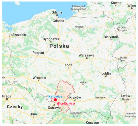
Figure 1.
Location of the investigated site (source: www.google.pl/maps (accessed on 20 November 2022)).
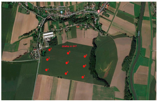
Figure 2.
Location of experiment points (source: www.googlemap.pl (accessed on 20 November 2022)).
3. Results and Discussion
In Table 2 there are presented values of some statistical measures of soil parameters used for calculation of saturated hydraulic conductivity by use of pedotransfer functions. Regarding texture, soil on the investigated site is classified as silt loam (SiL). Effective diameter d10 varied from 1.7·10−3 to 3.0·10−3 mm, d20 between 4.5·10−3 and 8.0·10−3 mm, while d50 between 2.8·10−3 mm and 3.8·10−2 mm. Values of organic matter fluctuated between 0.85 and 1.35%, while total porosity between 0.394 and 0.481. Bulk density attained values between 1.41 and 1.57 Mg·m−3. Values of saturated hydraulic conductivity Ks for analyzed points fluctuated between 3.25·10−2 and 8.72·10−2 m·day−1.
Table 2.
Statistical values of parameters for determination of saturated hydraulic conductivity by means of thepedotransfer functions.
Table 3 presents some statistical measures for saturated hydraulic conductivity determined by one of the fifteen pedotransfer functions. Generally, the obtained mean values were between 9.10·10−4 and 4.59·100 m·day−1.
Table 3.
Statistical parameters of the saturated hydraulic conductivity obtained for the chosenpedotransfer functions.
The analysis of variance was introduced in Table 4, while Table 5 presents statistically uniform groups regarding statistical essentiality. Method 13 (Fournivaland Wilson) showed statistically essential difference in relation to the other methods. In turn, between method 9 (Seelheim) and 14 (multiple regression) there is no statistically essential difference. Between method 14 (multiple regression) and the remaining following methods there is no statistical essential difference.
Table 4.
Analysis of variance.
Table 5.
Analysis of essential differences between results of determination by means of thepedotransfer functions.
In Table 6 there are presented results of statistical analysis of comparison of results obtained by means of field direct methods with the ones obtained by means of the chosen pedotransfer methods. The results show that the method 1 (Hazen), 3 (USBR), 4 (Saxton), 7 (Tezaghi), 8 (Chapuis), 9 (Seelheim), 10 (Chapuis-NAVFAC, 12 (Slichter), 13 (Furnival) and 14 (multiple regression) gave statistically essential differences in relation to the results obtained by means of the field method. Comparing, in turn, percentage differences, the least one showed method 5 (Kozeny-Carman, underestimation attaining 1.4%), and the highest showed method 13 (Furnival and Wilson, overestimation attained as many as 6036.4%).
Table 6.
Values of t-Student test between results obtained by means of the pedotransferfunctionswiththe ones obtained by means of measured data.
For the purpose to choose the best function simulating saturated hydraulic conductivity for the loess soil, the various model efficiency measures were used (Table 7). Values of correlation coefficient for pedotransfer functions fluctuated between 0.059 and 0.708.Only for methods 2nd (Hazen-Tkaczukowa), 4th (Saxton), 10th (NAVFAC) and 15th (ANN) coefficients were statistically essential for confidence level0.01.The best accordance with the field double-ring method regarding correlation coefficient had the 15th (ANN) method, while the most abandoning ones were 11th (Sauerbrej) and 12th (Slichter) functions. Results obtained for showed that maximum underestimation attained 2.18·10−2, for 15th (ANN) function, while little overestimation took place for 11th (Sauerbrej) function. Mean percentage error shows good results of estimation for 2nd (Hazen-Tkaczukowa) function. Its value was 6.2%. Extreme bad adjustment had 13th (Furnival and Wilson) (as many as −5774.6%) function. Root of mean square error attained the highest value for 13th (Furnival and Wilson) function(3.99·100·100 m·day−1). The best results attained 15th (ANN) function. Analysis of homogeneity of mean values (Table 4) using the Tukey’s test showed that the 13th (Furnival and Wilson) method differed statistically in comparison to other functions (Table 8). Functions 9th (Seelheim) and 14th (MRA) did not differ between them and differed statistically from the remaining methods.
Table 7.
Model efficiency measures.
Table 8.
Values of parameters of spatial distribution.
4. Conclusions
- The LSD analysis showed that the Fournival and Wilson method, based on texture and total porosity differs statistically for investigated site from the other methods. In turn, between the Seelheim (based on texture only) and multiple regression methods there is not a statistical difference. Between the Seelheim method and the other ones there are not a statistically essential difference;
- The t-Student analysis showed that the methods: Hazen, USBR, Saxton, Seelheim (based only on texture), Chapuis, NAVFAC, Furnival and Wiliam, multiple regression (based on texture and total porosity), and Slichter and Tezaghi (based on texture, total porosity and water properties)gave statistically essential differences in comparison to the results obtained by the field method. The remaining method does not differ statistically from the field method;
- Comparing the percentage differences, the lowest showed the Kozeny-Carman method, in which underestimation in relation to the field method was 1.4%. In turn, the highest difference was in the case of the Furnival and Wilson, in which overestimation was as many as 5.4%. The lowest differences were in the case of the methods where total porosity was taken into account;
- The highest spatial variability was for the Hazen and Tkaczukowa methods, where variability coefficient was 123.6%. In turn, the artificial neural network method was characterized by a lack of variability.
Author Contributions
Conceptualization, A.P. and M.R.; methodology, A.P. and M.R.; validation, E.K., L.L.; formal analysis, M.R.; resources M.R. and E.K.; writing—original draft preparation, M.R. and A.P.; writing—review and editing, A.P. and M.R.; supervision, E.K. and L.L.; project administration, A.P.; funding acquisition, A.P. and E.K. All authors have read and agreed to the published version of the manuscript.
Funding
The publication was co-financed from the subsidy granted to the Cracow University of Economics—Project nr 28/GGR/2021/POT.
Institutional Review Board Statement
Not applicable.
Informed Consent Statement
Not applicable.
Conflicts of Interest
The authors declare no conflict of interest.
References
- Halecki, W.; Kruk, E.; Ryczek, M. Loss of top soil and soil erosion by water in agricultural areas: A multi-criteria approach for various land use scenarios in the Western Carpathians using a SWAT model. Land Use Policy 2018, 73, 363–372. [Google Scholar] [CrossRef]
- Wang, X.; Zhao, X.; Zhang, Z.; Yi, L.; Zuo, L.; Wen, Q.; Liu, F.; Xu, J.; Hu, S.; Liu, B. Assessment of soil erosion change and its relationships with land use/cover change in China from the end of the 1980s to 2010. Catena 2016, 137, 256–268. [Google Scholar] [CrossRef]
- Cadaret, E.M.; McGwire, K.C.; Nouwakpo, S.K.; Weltz, M.A.; Saito, L. Vegetation canopy cover effects on sediment erosion processes in the Upper Colorado River Basin Mancos Shale formation, Price, Utah, USA. Catena 2016, 147, 334–344. [Google Scholar] [CrossRef]
- Cao, T.; She, D.; Zhang, X.; Yang, Z.; Wang, G. Pedotransfer functions developed for calculating soil saturated hydraulic conductivity in check dams on the Loess Plateau in China. Vadose Zone J. 2022, 21, 20217. [Google Scholar] [CrossRef]
- Evrarda, O.; Nordb, G.; Cerdanc, O.; Souchère, V.; Le Bissonnais, Y.; Bonté, P. Modelling the impact of land use change and rainfall seasonality on sediment export from an agricultural catchment of the northwestern European loess belt. Agric. Ecosyst. Environ. 2010, 138, 83–94. [Google Scholar] [CrossRef]
- Lia, P.; Mua, X.; Holdenb, J.; Wud, Y.; Irvineb, B.; Wanga, F.; Gaoa, P.; Zhaoa, G.; Suna, W. Comparison of soil erosion models used to study the Chinese Loess Plateau. Earth-Sci. Rev. 2017, 170, 17–30. [Google Scholar] [CrossRef]
- Yang, G.; Xu, Y.; Huo, L.; Wang, H. Analysis of Temperature Effect on Saturated Hydraulic Conductivity of the Chinese Loess. Water 2022, 14, 1327. [Google Scholar] [CrossRef]
- Li, J.T.; Wang, J.J.; Zeng, D.H.; Zhao, S.Y.; Huangb, W.L.; Sunc, X.K.; Hu, J. The influence of drought intensity on soil respiration during and after multiple drying-rewetting cycles. Soil Biol. Biochem. 2018, 127, 82–89. [Google Scholar] [CrossRef]
- Boroń, K.; Klatka, S.; Ryczek, M.; Zając, E. Reclamation and cultivation of Cracow Soda plant Lagoons. In Construction for Sustainable Environment; Sarsby, R., Meggyes, T., Eds.; CRC Press Taylor & Francis Group: London, UK, 2010; pp. 245–250. [Google Scholar]
- Daliakopoulos, I.N.; Tsanis, I.; Koutroulis, A.; Kourgialas, N.; Varouchakis, A.; Karatzas, G.; Ritsema, C. The threat of soil salinity: A European scale review. Sci. Total Environ. 2016, 573, 727–739. [Google Scholar] [CrossRef]
- Mau, Y.; Porporato, A. A dynamical system approach to soil salinity and sodicity. Adv. Water Resour. 2015, 83, 68–76. [Google Scholar] [CrossRef]
- Mau, Y.; Porporato, A. Optimal control solutions to sodic soil reclamation. Adv. Water Resour. 2016, 91, 37–45. [Google Scholar] [CrossRef]
- Rath, K.M.; Maheshwari, A.; Rousk, J. The impact of salinity on the microbial response to drying and rewetting in soil. Soil Biol. Biochem. 2017, 108, 17–26. [Google Scholar] [CrossRef]
- Wanga, L.; Shi, J.; Zuo, Q.; Zhang, W.; Zhuc, X. Optimizing parameters of salinity stress reduction function using the relationship between root-water uptake and root nitrogen mass of winter wheat. Agric. Water Manag. 2012, 104, 142–152. [Google Scholar] [CrossRef]
- Achary, M.S.; Satpathy, K.; Panigrahi, S.; Mohanty, A.; Padhi, R.; Biswas, S.; Prabhu, R.; Vijayalakshmi, S.; Panigrahy, R. Concentration of heavy metals in the food chain components of the nearshore coastal waters of Kalpakkam, southeast coast of India. Food Control 2017, 72, 232–243. [Google Scholar] [CrossRef]
- VanOosten, M.J.; Maggio, A. Functional biology of halophytes in the phytoremediation of heavy metal contaminated soils. Environ. Exp. Bot. 2015, 111, 135–146. [Google Scholar] [CrossRef]
- Klatka, S.; Malec, M.; Ryczek, M.; Kruk, E.; Zając, E. Evaluation of retention ability of chosen industrial wastes. Acta Sci. Pol. Form. Circumiectus 2016, 15, 53–60. [Google Scholar] [CrossRef]
- Zając, E.; Zarzycki, J.; Ryczek, M. Degradation of peat surface on an abandoned post-extracted bog and implications for re-vegetation. Appl. Ecol. Environ. Res. 2018, 16, 3363–3380. [Google Scholar] [CrossRef]
- El-Hames, A.S. An empirical method for peak discharge prediction in ungauged arid and semi-arid region catchments based on morphological parameters and SCS curve number. J. Hydrol. 2012, 456–457, 94–100. [Google Scholar] [CrossRef]
- Sanzeni, A.; Colleselli, F.; Grazioli, D. Specific surface and Hydraulic Conductivity of Fine-Grained Soils. J. Geotech. Geoenvironmental Eng. 2013, 139, 892. [Google Scholar] [CrossRef]
- Tyagi, J.V.; Mishra, S.K.; Singh, R.; Singh, V.P. SCS-CN based time-distributed sediment yield model. J. Hydrol. 2008, 352, 388–403. [Google Scholar] [CrossRef]
- USDA. Urban Hydrology for Small Watersheds; Technical Release, 55; U.S. Department of Agriculture, Natural Resources Conservation Service, Conservation Engineering Division: Washington, DC, USA, 1986. [Google Scholar]
- Tietje, O.; Hennings, V. Accuracy of the saturated hydraulic conductivity prediction by pedo-transfer functions compared to the variability within FAO textural classes. Geoderma 1996, 69, 71–84. [Google Scholar] [CrossRef]
- Abdelbaki, A.M. Selecting the most suitable pedotransfer functions for estimating saturated hydraulic conductivity according to the available soil inputs. Ain Eng. J. 2021, 12, 2603–2615. [Google Scholar] [CrossRef]
- Ke, X.; Liu, P.; Wang, W.; Li, J.; Niu, F.; Gao, Z.; Kong, D. Spatial variability of the vertical saturated hydraulic conductivity of sediments around typical thermokarst lakes. Geoderma 2023, 429, 116230. [Google Scholar] [CrossRef]
- Klatka, S.; Ryczek, M.; Boroń, K. Water characteristics curves of soils degraded by coal mine industry. Ochr. Sr. I Zasobów Nat. 2010, 42, 130–135. [Google Scholar]
- Klatka, S.; Malec, M.; Ryczek, M. Analysis of Spatial Variability of Selected Soil Properties in the Hard Coal Post-Mining Area. J. Ecol. Eng. 2019, 20, 185–193. [Google Scholar] [CrossRef]
- Regalado, C.M.; Muñoz-Carpena, R. Estimating the saturated hydraulic conductivity in a spatially variable soil with different permeameters: A stochastic Kozeny–Carman relations. Soil Tillage Res. 2004, 77, 189–202. [Google Scholar] [CrossRef]
- Rienzner, M.; Gandolfi, C. Investigation of spatial and temporal variability of saturated soil hydraulic conductivity at the field-scale. Soil Tillage Res. 2014, 135, 28–40. [Google Scholar] [CrossRef]
- Jabro, J. Estimation of saturated conductivity of solis from particle size distribution and bulk density date. Trans. Am. Soc. Agric. Eng. 1992, 35, 557–560. [Google Scholar] [CrossRef]
- Carrier, D. Goodbye, Hazen; Hello, Kozeny-Carman, Technical notes. J. Geotech. Geoenvironmental Eng. 2003, 129, 1054–1056. [Google Scholar] [CrossRef]
- Chapuis, R. Predicting the Saturated Hydraulic Conductivity of Natural Soils. Geotech. News 2008, 47–50. [Google Scholar]
- Kruk, E.; Klapa, P.; Ryczek, M.; Ostrowski, K. Comparison of the USLE to pographical factor parameter generated by various DE Melaboration methods on loesss lopes. Remote Sens. 2020, 12, 3540. [Google Scholar] [CrossRef]
- Odong, J. Evaluation of empirical formulae for determination of hydraulic conductivity based on grain-size analysis. J. Am. Sci. 2007, 3, 54–60. [Google Scholar]
- Parylak, K.; Zięba, Z.; Bułdys, A.; Witek, K. The verification of determining a permeability coefficient of non-cohesive soil based on empirical formulas including its microstructure. Acta Sci. Pol. 2013, 12, 43–51. [Google Scholar]
- Salarashayeri, A.F.; Siosemarde, M. Prediction of Soil Hydraulic Conductivity from Particle Size Distribution Analysis. World Acad. Sci. Eng. Technol. 2012, 6, 16–20. [Google Scholar]
- Twardowski, K.; Drożdżak, R. Indirect methods of estimating hydraulic properties of grounds. Wiert. Naft. Gaz 2006, 23, 477–486. [Google Scholar]
- Bilardi, S.; Ielo, D.; Moraci, N. Predicting the Saturated Hydraulic Conductivity of Clayey Soil sand Clayey or Silty Sands. Geosciences 2020, 10, 393. [Google Scholar] [CrossRef]
- Chapuis, R.P. Predicting the saturated hydraulic conductivity of soils: A review Bulletin of Engineering Geology and the Environment. Bull. Eng. Geol. Environ. 2012, 71, 401–434. [Google Scholar] [CrossRef]
- Mbonimpa, M.; Aubertin, M.; Chapuis, R.P.; Bussiére, B. Practical pedotransfer functions for estimating the saturated hydraulic conductivity. Geotech. Geol. Eng. 2002, 20, 235–259. [Google Scholar] [CrossRef]
- Nash, J.E.; Sutcliffe, J.V. River flow forecasting through conceptual models. Part I. A Discussion of Principles. J. Hydrol. 1970, 10, 282–290. [Google Scholar] [CrossRef]
- Patil, N.G.; Singh, S.K. Pedotransfer functions for estimating soil hydraulic properties: A review. Pedosphere 2016, 26, 417–430. [Google Scholar] [CrossRef]
- Sarangi, A.; Bhattacharya, A.K. Comparison of artificial neural network and regression models for sediment loss prediction from Banha watershed in India. Agric. Water Manag. 2005, 78, 195–208. [Google Scholar] [CrossRef]
- Sobieraj, J.A.; Elsenbeer, H.; Vertessy, R.A. Pedotransfer functions for estimating saturated hydraulic conductivity: Implications for modeling storm flow generation. J. Hydrol. 2001, 251, 202–220. [Google Scholar] [CrossRef]
- Tiwari, A.K.; Risse, L.M.; Nearing, M.A. Evaluation of WEPP and its comparison with USLE and RUSLE. Trans. ASAE 2000, 43, 1129–1135. [Google Scholar] [CrossRef]
- Bouma, J. Using soil survey data for quantitative land evaluation. In Advances in Soil Science; Stewart, B.A., Ed.; Springer: Berlin/Heidelberg, Germany, 1989; Volume 9, pp. 177–213. [Google Scholar]
- Van Looy, K.; Bouma, J.; Herbst, M.; Koestel, J.; Minasny, B.; Mishra, U.; Montzka, C.; Nemes, A.; Pachepsky, Y.A.; Padarian, J.; et al. Pedotransfer functions in Earth system science: Challenges and perspectives. Rev. Geophys. 2017, 55, 1199–1256. [Google Scholar]
- Briggs, L.J.; Lane, J.W.M. The moisture equivalents of soils. U.S. In Department of Agriculture Bureau of Soils. Bulletin; U.S. Government Printing Office: Washington, DC, USA, 1907; p. 23. [Google Scholar]
- Cosby, B.J.; Hornberger, G.M.; Clapp, R.B.; Ginn, T.R. A statistical exploration of the relationships of soil moisture characteristic to the physical properties of soils. Water Resour. Res. 1984, 20, 682–690. [Google Scholar] [CrossRef]
- Rawls, W.J.; Brakensiek, D.L.; Soni, B. Agricultural management effects on soil water processes. Part I: Soil water retention and Green and Ampt infiltration parameters. Trans. ASAE 1983, 26, 1747–1752. [Google Scholar]
- Saxton, K.E.; Rawls, W.J. Soil water characteristic estimates by texture and organic matter for hydrologic solutions. Soil Sci. Soc. Am. J. 2006, 70, 1569–1578. [Google Scholar]
- De Lannoy, G.J.M.; Koster, R.D.; Reichle, R.H.; Mahanama, S.P.P.; Liu, Q. An updated treatment of soil texture and associated hydraulic properties in a global land modeling system. J. Adv. Model. Earth Syst. 2014, 6, 957–979. [Google Scholar]
- Ditzler, C.; Scheffe, K.; Monger, H.C. ; Soil Science Division Staff. Soil Survey Manual; USDA Handbook No. 18; USDA: Washington DC, USA, 2017; 603p. [Google Scholar]
- Rawles, W.; Brakensiek, D. Estimating soil water retention from soil properties. J. Irrig. Drain. Div. 1982, 108, 166–171. [Google Scholar] [CrossRef]
- Wösten, J.H.M.; Lilly, A.; Nemes, A.; LeBas, C. Development and use of a database of hydraulic properties of European soils. Geoderma 1999, 90, 169–185. [Google Scholar]
- Pisarczyk, S. Elementy Budownictwa Ochrony Środowiska; Wydawnictwo Oficyna Wydawnicza Politechniki Warszawskiej: Warszawa, Poland, 2008; p. 185. [Google Scholar]
- Vukovic, M.; Soro, A. Determination of Hydraulic Conductivity of Porous Media from Grain Size Composition; Water Resources Publications: Littleton, CO, USA, 1992. [Google Scholar]
- Saxton, K.E.; Rawls, W.J.; Romberger, J.S.; Papendick, R.I. Estimating Generalized Soil-Water Characteristics from Texture. Soil Sci. Soc. Am. J. 1986, 50, 1031–1035. [Google Scholar] [CrossRef]
- Pazdro, Z.; Kozerski, B. Hydrologia Ogólna; Wydawnictwo Geologiczne: Warszawa, Poland, 1990. [Google Scholar]
- Kozerski, B. Zasady obliczeń hydraulicznych ujęć wód podziemnych. In Wytyczne Okreśłenia Współczynnika Filtracji Metodami Pośrednimii Laboratoryjnymi; Wydawnictwo Geologiczne: Warszawa, Poland, 1977. [Google Scholar]
- Sezer, A.; Göktepe, A.B.; Altun, S.; Bassiliades, N. Estimation of the permeability of granular soils using neuro-fuzzy system. In Proceedings of the Workshops of the 5th IFIP Conference on Artificial Intelligence Applications & Innovations (AIAI-2009), Thessaloniki, Greece, 23–25 April 2009. [Google Scholar]
- Myślińska, E. Laboratoryjne Badania Gruntów; Wydawnicto Naukowe: PWN Warszawa, Poland, 1998. [Google Scholar]
- Wösten, J.H.M.; Finke, P.A.; Jansen, M.J.W. Comparison of class and continuous pedotransfer functions to generate soil hydraulic characteristics. Geoderma 1995, 66, 227–237. [Google Scholar] [CrossRef]
- Ryczek, M.; Kruk, E.; Malec, M.; Klatka, S. Comparison of pedotransfer functions for the determination of saturated hydraulic conductivity coefficient. Ochr. Sr. I Zasobów Nat. Environ. Prot. Nat. Resour. 2017, 28, 25–30. [Google Scholar]
- Vereecken, H.; Maes, J.; Feyen, J.; Darius, P. Estimating the soil moisture retention characteristic from texture, bulk density, and carbon content. Soil Sci. 1989, 148, 389–403. [Google Scholar]
- Kruk, E.; Malec, M.; Klatka, S.; Brodzińska-Cygan, A.; Kołodziej, J. Pedotransfer function for determining saturated hydraulic conductivity using artificial neural network (ANN). Acta Sci. Pol. Form. Circumiectus 2017, 16, 115–126. [Google Scholar] [CrossRef]
- Rahnama, M.B.; Barani, G.A. Application of rainfall-runoff models to Zard river catchments. Am. J. Environ. Sci. 2005, 1, 86–89. [Google Scholar]
- Kondracki, J. Geografia Regionalna Polski; Wydawnictwo Naukowe PWN: Warszawa, Poland, 2000. [Google Scholar]
- Weynants, M.; Vereecken, H.; Javaux, M. Revisiting Vereecken pedotransfer functions: Introducing a closed-form hydraulic model. Vadose Zone 2009, 81, 86. [Google Scholar]


Disclaimer/Publisher’s Note: The statements, opinions and data contained in all publications are solely those of the individual author(s) and contributor(s) and not of MDPI and/or the editor(s). MDPI and/or the editor(s) disclaim responsibility for any injury to people or property resulting from any ideas, methods, instructions or products referred to in the content. |
© 2023 by the authors. Licensee MDPI, Basel, Switzerland. This article is an open access article distributed under the terms and conditions of the Creative Commons Attribution (CC BY) license (https://creativecommons.org/licenses/by/4.0/).