Quantitative Evaluation of Runoff Simulation and Its Driving Forces Based on Hydrological Model and Multisource Precipitation Fusion

Abstract

The hydrological cycle across the source regions of the Yellow River (SRYR) affects water supply for 324 million people across the Yellow River basin (YRB), and the scarcity of meteorological stations leads to great challenges for the estimation of hydrologic and energy balance. Therefore, our work employs multisource precipitation products across the YRB to develop a new integrated precipitation product with the optimized Bayesian mean algorithm (OBMA). It investigates the performance and hydrological utility of the optimal Bayesian integrated precipitation product (OBIPP). This study found that the OBIPP improved by 14.08% in overall performance relative to the optimal precipitation product across the SRYR, respectively. Meanwhile, the variable infiltration capacity (VIC) model, driven by daily OBIPP, can drastically improve the accuracy of runoff simulation compared with other precipitation products across the SRYR. According to the VIC model driven by daily OBIPP, the average precipitation and runoff depth across the SRYR were approximately 621 mm and 64 mm from 2001 to 2019, respectively, showing a spatial trend increasing from northwest to southeast. Overall, OBIPP is characterized by smaller uncertainty of simulation and higher simulation performance across the SRYR, which should provide a scientific basis for accurate prediction and assessment of water resources in areas where meteorological data are scarce.

1. Introduction

As one of the world’s significant natural and strategic economic resources, water resources play a pivotal role in maintaining and promoting sustainable socioeconomic development [1]. Meanwhile, precipitation and runoff are the main parts of the hydrological cycle. The abundance of regional water resources is determined by high and low rainfall, which affects many physical, chemical, and biological processes in natural and social systems. Runoff change represents a fundamental direction for assessing water resources as needed for strategic planning and management. However, in the context of climate change and rapid urbanization, the reliability of precipitation information restricts the accuracy of quantitative research on runoff simulations [2].

Currently, there are various forecast precipitation products, including ground-based observations, ground-based radar products, satellite remote sensing products, and reanalysis products. Ground-based observations have very high accuracy. However, under the scarcity of meteorological stations and precipitation heterogeneity, forecast precipitation products are unrepresentative of regions with insufficient meteorological data. They cannot truly reflect the spatial distribution pattern of rainfall [3]. The effective detection radius of ground-based radar products can reach approximately 250 km. However, the detection accuracy is affected by the quantitative relationship between radar reflectivity and precipitation intensity, the radius variation of raindrops during the landing process, beam blocking, and noise interference [4]. Compared with ground-based observations and ground-based radar products, satellite, remote sensing, and reanalysis precipitation products have the advantages of wide coverage, time continuity, and high spatial resolution, and gradually become an important way to obtain precipitation data in data-deficient or no-data areas [5]. However, precipitation is often spatially and temporally heterogeneous due to topography, geographic location, atmospheric physical motion, and underlying surface changes. Hence, precipitation products from single sourcing have significant uncertainty. How to develop multisource precipitation integrated algorithm to effectively integrate the advantages of different precipitation products to obtain more accurate precipitation information is a hot topic of current research.

Multisource integrated precipitation products can reduce the ambiguity of meteorological and hydrological assessments to a certain extent. Due to the uncertainty of a single precipitation product, there is a multitude of integrated methods to improving the effectiveness of a single precipitation product to a large extent, including the multi-model ensemble [6], average method of eliminating outliers [7], geographically weighted regression [8], multivariable geostatistical methods [9], and Bayesian mean algorithm (BMA) [10,11]. However, most of the multisource precipitation products integrate only achieve the integration of a single precipitation product and ground-based observations [12,13]. There are also some studies on the linear integration of multisource precipitation products and ground-based observations [14,15], and only a few studies have realized the nonlinear integration of multisource precipitation products. Among them, the Bayesian mean algorithm (BMA) is a more advanced ensemble weighting algorithm that uses ground-based observations to obtain the optimal weights of different products. Compared with linear or nonlinear methods, BMA provides a more reasonable description of forecast ambiguity, representing changes between and within models. However, BMA relies on all ensemble forecast members, and poor regional simulation of a particular forecast member can affect the overall forecast results. Therefore, this study aims to develop an optimized Bayesian mean algorithm (OBMA) to obtain the precipitation information by integrating multisource precipitation products of long time sequence to fill the gap in precipitation in regions without data.

The Yellow River basin (YRB) is one of the most fragile watershed systems affected by global warming [16]. One of the fundamental sources of this vulnerable and even suffering state is the temporal variability and uneven spatial distribution of precipitation [17]. For example, rainstorms and continuous rainfall are important factors for the frequent occurrence of geological disasters across the YRB, and at least 1/3 of landslide disasters in China occur in this area [18]. In addition, the distribution of meteorological stations in the source region of the Yellow River (SRYR) is seriously uneven, with extremely low density, and has poorly representative and discontinuous data sequences, which cannot meet the needs of hydrological simulations. In the SRYR, it had been reported that satellite remote sensing and reanalysis products have the potential to improve the quality of precipitation and runoff simulation [19,20,21].

In summary, the accuracy of spatialized precipitation information primarily affects hydrological simulation and forecasting. In addition, it is expected that only one or two products be considered, which may lead to uncertainty in forecast results. This study’s objective was to evaluate the optimal Bayesian integrated precipitation product (OBIPP) performance relative to other precipitation products. On this basis, we selected a typical SRYR to explore the simulation performance of the VIC model driven by daily OBIPP to provide scientific guidance and a decision basis for water resources assessment and management in related regions.

2. Materials and Methods

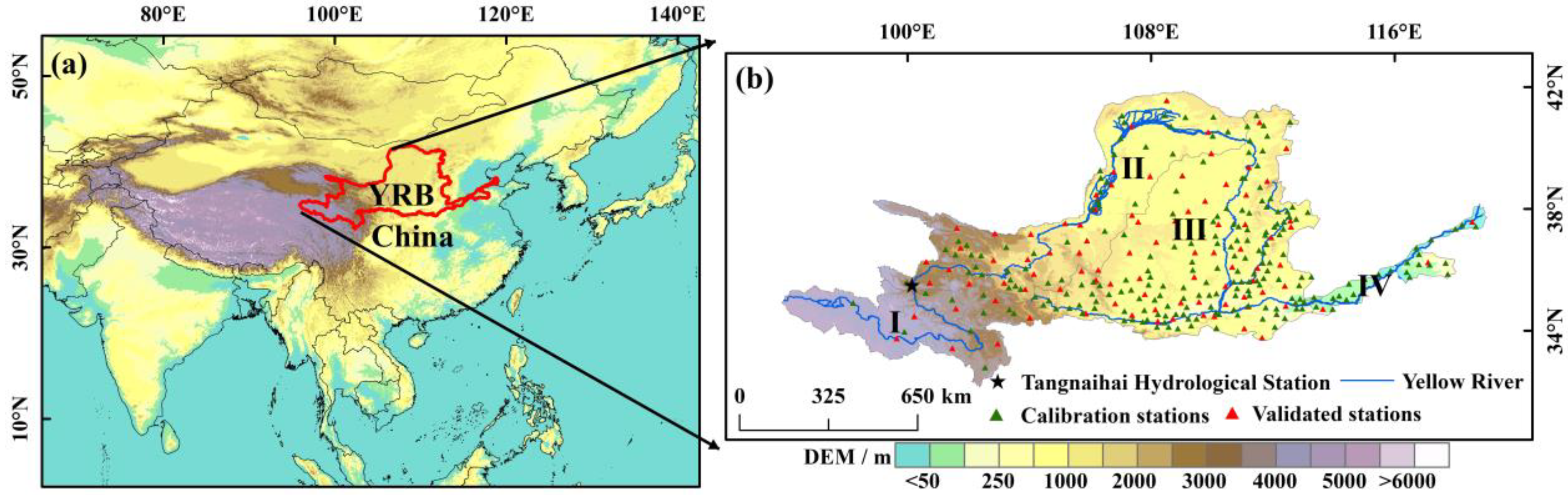
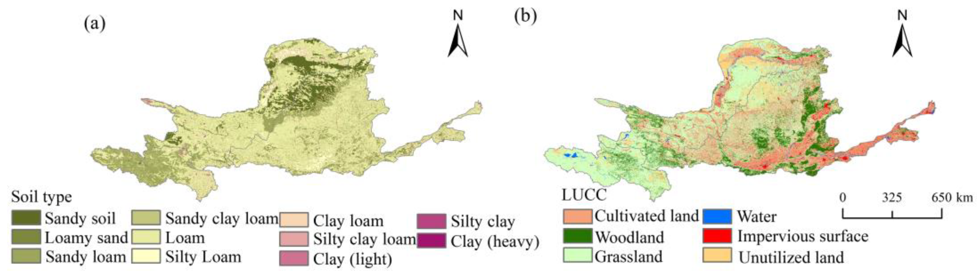
2.1. Study Area

The YRB (32°10′ N–41°50′ N, 95°53′ E–119°05′ E) (Figure 1), the fifth largest river around the world and the second longest river across China, is regarded as the “Mother River of China” [22]. The YRB covers approximately 12.6 × 1010 km² of farmland, supporting more than 9% of China’s total population and providing 16% of grain yield across China [3]. Originating on the Tibetan Plateau (TP), the YRB crosses the Inner Mongolia Plateau (IMP), Loess Plateau (LP), and North China Plain (NCP) to the east and finally flows into the Bohai Sea. The YRB belongs to the typical temperate monsoon climate, with high temperature, rain in summer, cold and dry in winter, uneven seasonal distribution of precipitation, and precipitation concentrated in summer, and July–August rainstorms are frequent. Based on the characteristics of the basin and the location of hydrological stations, the YRB is divided into four subregions (Figure 1).

2.2. Materials

Detailed information on meteorological elements were obtained from 312 meteorological stations from 2001 to 2019, including observed daily precipitation, maximum temperature, minimum temperature, average temperature, wind speed, duration of sunshine, and relative humidity, while daily observed runoff was obtained at the Tangnaihai (TNH) between 2001 and 2019 (Figure 1). These data have undergone strict quality control [23]. Among them, meteorological data were collected by the National Meteorological Science Data Center (http://data.cma.cn/ (accessed on 4 September 2021)), and runoff data were collected by the Yellow River Conservancy Commission of the Ministry of Water Resources (http://www.yrcc.gov.cn/ (accessed on 23 August 2022)), respectively.

Six single precipitation products (SPPs) were selected for integration and hydrological simulation, including CHIRPS, CPC, TRMM-3B42, GPM-IMERG, PERSIANN-CDR, and ERA5-LAND. Essential information about the products is shown in

Table 1. Multisource precipitation product information.

Precipitation Products	Abbreviation	Temporal Resolution	Spatial Resolution	Time Span	References
CHIRPS	CHIRPS	Day	0.05°	1981	Funk et al. (2015) [24]
CPC	CPC	Day	0.5°	1979	Xie et al. (2007) [25]
TRMM-3B42	TRMM	3 h	0.25°	1998	Huffman et al. (1997) [26]
GPM-IMERG	GPM	0.5 h	0.1°	2000	Huffman et al. (2014) [27]
PERSIANN-CDR	PERSIANN	Day	0.25°	1983	Sorooshian et al. (2000) [28]
ERA5-LAND	ERA	1 h	0.1°	1950	Hersbach et al. (2020) [29]

. CHIRPS (https://data.chc.ucsb.edu/products/ (accessed on 13 June 2022)) and CPC (https://psl.noaa.gov/data/gridded/ (accessed on 13 June 2022)) represent precipitation products integrated with satellite images and in situ precipitation. The data are optimized and quality controlled in combination with the terrain effect, forming a high accuracy and consistency precipitation product [24,25]. TRMM-3B42 (https://disc.gsfc.nasa.gov/datasets/ (accessed on 17 June 2022)) is a typical representative of current satellite remote sensing products, while GPM-IMERG (https://disc.gsfc.nasa.gov/ (accessed on 4 June 2022)) is the follow-up global satellite precipitation observation plan of TRMM led by NASA [26,27]. PERSIANN-CDR (https://www.ncei.noaa.gov/data/ (accessed on 21 May 2022)) uses the artificial neural network algorithm to estimate precipitation rates based on infrared brightness temperature data provided by geosynchronous satellites [28]. ERA5-LAND (https://cds.climate.copernicus.eu/ (accessed on 27 May 2022)) is a new generation of reanalysis product from the European Centre for Medium-Range Weather Forecasts, using IFS-Cycle4lr2 and the four-dimensional variational data assimilation system, as well as the radiometric variance bias correction technique, which systematically improves the quality of the dataset and increases the global average correlation coefficient from 0.67 to 0.77 in precipitation compared to the monthly average GPCP data [29]. Considering the difference in resolution between the different products and referring to previous studies, a bilinear interpolation was used to convert the six precipitation products to a 0.1° × 0.1° resolution [6].

The variable infiltration capacity (VIC) model also requires, as input, the digital elevation model (DEM), soil texture, and characteristic vegetation parameters. The digital elevation model, with a horizontal resolution of 90 m, which is used to extract the basin information, was obtained from Geospatial Data Cloud (http://www.gscloud.cn (accessed on 11 August 2022), Figure 1b). The soil texture of the SRYR is obtained from the 5′ Food and Agriculture Organization (FAO) dataset [30,31,32] (Figure 2a). It can be seen that most areas of the YRB are loam, and only northwest of the SRYR is sandy loam. Characteristic vegetation parameters are based on the 1 km remote sensing monitoring data of land-use and land-cover change (LUCC) across the YRB developed at the Resource and Environment Data Center of the Chinese Academy of Sciences (https://www.resdc.cn/ (accessed on 24 June 2022), Figure 2b). According to Figure 2, the cultivated land, woodland, grassland, water, impervious, and unutilized land across the YRB account for 26.27%, 13.15%, 47.54%, 1.74%, 3.17%, and 8.12% of the total area of the basin, respectively. The actual evapotranspiration was obtained using the ERA5-LAND with a horizontal resolution of 0.1°, and this actual evapotranspiration shows good applicability across the YRB [33].

2.3. Methods

The general flowchart of this research is presented in Figure 3. Firstly, the daily precipitation of 220 calibration stations from 2001 to 2019 was used to estimate the optimal weighted weights for the grid of calibration stations corresponding to six SPPs. BMA relies on all ensemble forecast members, and poor regional simulation of a particular forecast member can affect the overall forecast results. Therefore, Our research selects the OBIPP from 57 Bayesian integrated precipitation products (BIPP) based on the overall characteristics of simulations and observations. Secondly, OBIPP was evaluated for its precipitation simulation performance across the YRB relative to other precipitation products. Finally, a typical SRYR was selected to investigate the reliability and uncertainty of the OBIPP in hydrological simulations.

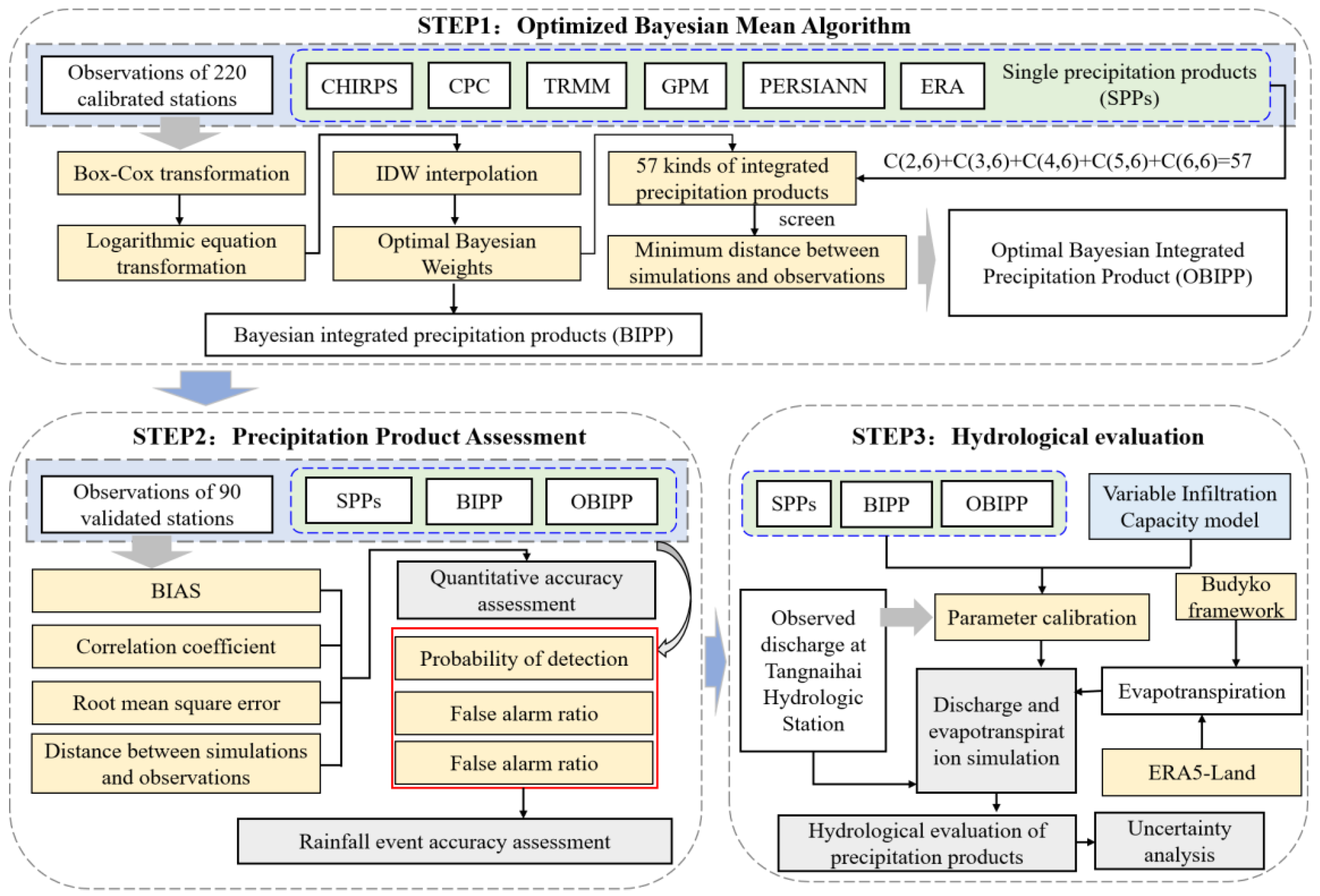
2.3.1. Optimized Bayesian Mean Algorithm (OBMA)

BMA is a statistical reprocessing method used earlier in hydrometeorological forecasting and uncertainty assessment. It relies on all ensemble forecast members rather than a single “optimal” forecast model and improves the forecast results by considering the uncertainty within multiple members [34]. Since BMA relies on all ensemble forecast members, poor regional simulation of a particular forecast member can affect the overall forecast results. Therefore, our research selects the OBIPP from 57 BIPP based on the overall characteristics of simulations and observations to obtain more accurate precipitation information of data-sparse regions.

Considering the monthly precipitation variation across the YRB, the optimal weights of BMA were calculated month by month. Let S be the daily precipitation, and R = [D, O] characterize the model input data (where D is the time sequence of simulations and O is the time sequence of observation). f = [f₁, f₂, …, f_n] are the outputs of each precipitation product. The probability density function of S can be obtained from the Bayesian total probability formula as follows [35]:

$$p\left(S\left|O\right.\right)={\displaystyle \sum _{n=1}^{n}p\left(f_n\left|O\right.\right)p_{\mathrm{k}}\left(S\left|f_n,O\right.\right)}$$

(1)

where p_k(S|f_n, O) is the probability density function of simulations (S) of the nth precipitation product (f_n) under observations (O); p(f_n|O) is the posterior probability density function of the nth precipitation product given the S at the specific calibration station. It represents the advantages and disadvantages of the S of the six precipitation products, and the sum of the posterior probabilities of the six precipitation products is 1. The BMA uses the posterior probabilities as weights to weigh the p(f_n|O) under different precipitation products, and the models with higher precipitation product accuracy receive relatively larger weights.

Then, the BMA can prefer the corresponding weights by the relative contribution of the deviation correction effect of each precipitation product. The final output precipitation product time sequence is the weighted average result of each precipitation product time sequence when the precipitation obeys normal distribution. The formula of the BMA can be derived based on the assumption of normal linear distribution:

$$E\left(S\left|O\right.\right)={\displaystyle \sum _{n=1}^{n}p\left(f_n\left|O\right.\right)E\left[g\left(S\left|f_n,{\sigma }_n^2\right.\right)\right]}={\displaystyle \sum _{n=1}^n{w}_n{f}_n}$$

(2)

where g(S|f_n, ${\sigma }_n^2$) is a normal distribution with mean f_n and variance; E is the expectation of the function; w_n is the weights of the nth precipitation product.

The parameter of BMA generation is set as θ = {w_n, ${\sigma }_n^2$, n = 1, 2, …, n}. Firstly, the observations and simulations of each precipitation product are transformed normally using the Box–Cox function, and then the logarithmic form of the θ likelihood function is expressed:

$$l\left(\theta \right)=\mathit{log}\left(p\left(S\left|O\right.\right)\right)=\mathit{log}\left({\displaystyle \sum _{n=1}^n{w}_{k}g\left(S\left|f_k,{\sigma }_k^2\right.\right)}\right)$$

(3)

Formula (3) is challenging to obtain the solution directly. Hence, the expectation maximization (EM) algorithm can be adopted to obtain the convergent maximum likelihood value, so as to obtain the numerical solution of θ = {w_n, ${\sigma }_n^2$, n = 1, 2, …, n}. In the EM algorithm, the hidden variable $Z_n^t$ is defined first, and the specific iterative steps are as follows:

(1)

Initialization (our research set iter = 0), given the initial weights and variances of each precipitation product:

$$w_{n0}=1/n,{\sigma }_{k0}^2={\displaystyle \sum _{n=1}^n{\displaystyle \sum _{t=1}^{NT}{\left(O^t-f_n^t\right)}^2/\left(nNT\right)}}$$

(4)

where NT is the length of the time sequence; ot and $f_n^t$ are the observations at t time and the simulations of the nth precipitation product, respectively.

(2)

Calculate the likelihood values of the initial parameters:

$$l_0\left(\theta \right)={\displaystyle \sum _{t=1}^{NT}\mathit{log}}\left({\displaystyle \sum _{n=1}^n\left[w_{n0}\mathit{g}\left(S\left|f_k^t,{\sigma }_{n0}^2\right.\right)\right]}\right)$$

(5)

(3)

Let Iter = Iter + 1 and calculate the iterative value of the hidden variable:

$$z_{k\left(Iter\right)}^t=g\left(S\left|f_n^t,{\sigma }_{n\left(Iter-1\right)}^2\right.\right)/{\displaystyle \sum _{n=1}^{n}g}\left(S\left|f_n^t,{\sigma }_{n\left(Iter-1\right)}^2\right.\right)$$

(6)

(4)

Calculation of weights for each precipitation product based on $Z_n^t$:

$$w_{n\left(Iter\right)}={\displaystyle \sum _{t=1}^{NT}{z}_{n\left(Iter\right)}^t/NT}$$

(7)

(5)

Recalculate the deviation of each precipitation product:

$${\sigma }_{n\left(Iter\right)}^2={\displaystyle \sum _{t=1}^{NT}\left[z_{n\left(Iter\right)}^t{\left(o^t-f_n^t\right)}^2\right]/{\displaystyle \sum _{t=1}^{NT}{z}_{n\left(Iter\right)}^t}}$$

(8)

(6)

Calculate the likelihood values of the parameters at the nth iteration state:

$$l_{Iter}\left(\theta \right)={\displaystyle \sum _{t=1}^{NT}\mathit{log}\left({\displaystyle \sum _{n=1}^n\left[w_{n\left(Iter\right)}g\left(S\left|f_n^t,{\sigma }_{n\left(Iter\right)}^2\right.\right)\right]}\right)}$$

(9)

(7)

Convergence check: if the l_Iter(θ) − l_Iter−1(θ) is less than the preset threshold (set to 0.0001 in this study) or the number of iterations exceeds the preset upper limit (10,000 iterations in this study), the iteration stops. Otherwise, return to step (3).

(8)

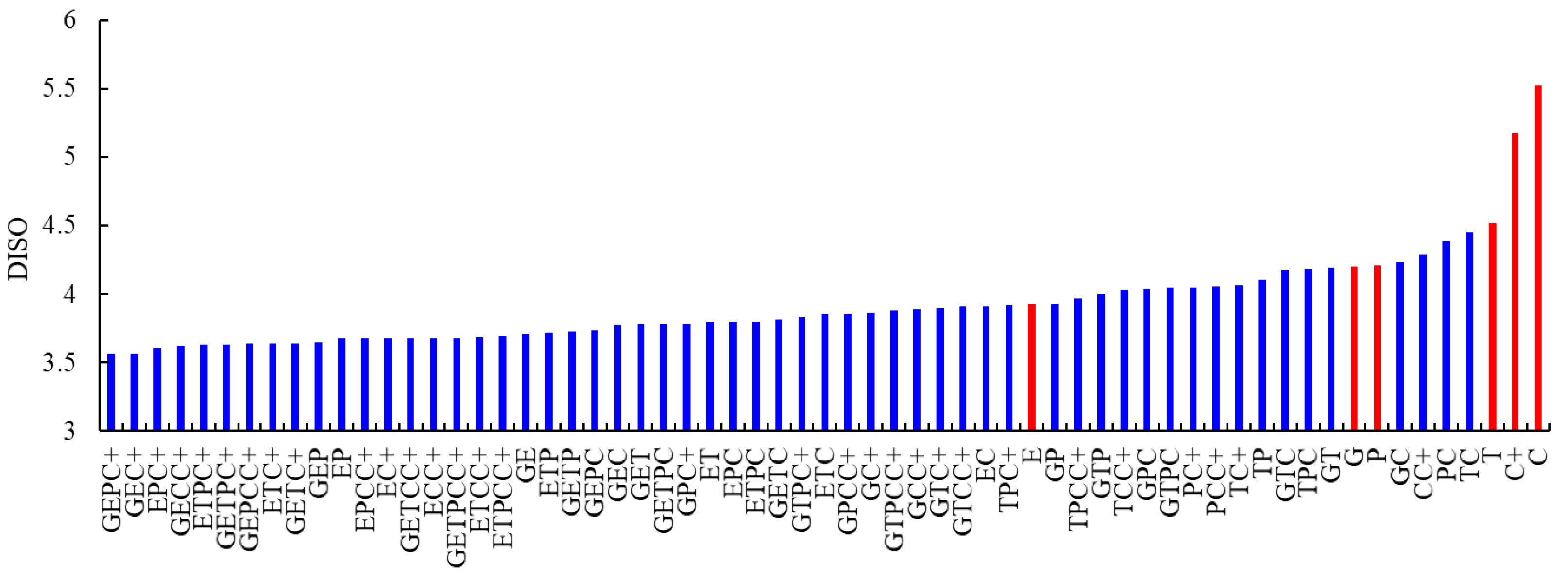
The optimal weights of each precipitation product can be obtained by steps (1) to (7). Based on the optimal weights, our research combined and integrated six SPPs to obtain 57 daily BIPPs.

$$C\left(2,6\right)+C\left(3,6\right)+C\left(4,6\right)+C\left(5,6\right)+C\left(6,6\right)=57$$

(10)

(9)

The distance between simulations and observations (DISO) of 57 daily BIPP is evaluated by calibration stations, and the minimum DISO is selected to obtain a new daily precipitation product. Our research overcomes the limitation that traditional BMA is affected by SPPs. The DISO calculation formula is as follows [36]:

$$BIAS=\frac{{\displaystyle \sum _{\mathrm{i}=1}^{\mathrm{n}}\left(S_{\mathrm{i}}-G_{\mathrm{i}}\right)}}{{\displaystyle \sum _{\mathrm{i}=1}^{\mathrm{n}}{G}_{\mathrm{i}}}}$$

(11)

$$CC=\frac{{\left[{\displaystyle \sum _{\mathrm{i}=1}^{\mathrm{n}}\left(S_{\mathrm{i}}-\overline{S}\right)\times }\left(G_i-\overline{G}\right)\right]}^2}{{\displaystyle \sum _{\mathrm{i}=1}^{\mathrm{n}}{\left(S_{\mathrm{i}}-\overline{S}\right)}^2\times {\displaystyle \sum _{\mathrm{i}=1}^{\mathrm{n}}{\left(G_{\mathrm{i}}-\overline{G}\right)}^2}}}$$

(12)

$$RMSE=\sqrt{\frac{1}{n}{\displaystyle \sum _{i=1}^n{\left(S_i-G_i\right)}^2}}$$

(13)

$$DISO=\sqrt{BIA{S}^2+{(CC-1)}^2+NRMS{E}^2}$$

(14)

where BIAS is used to express the bias between simulations and observations; CC is to describe the degree of agreement between simulations and observations; RMSE or NRMSE is used to show the magnitude of the error between simulations and observations; DISO is used to describe the overall characteristics of simulations relative to observations; n represents the length of the time sequence; G_i (S_i) represents the ith observations (simulations); $\overline{G }\left(\overline{S}\right)$ represents the average of observations (simulations); NRMSE is RMSE divided by $\overline{G}$.

2.3.2. VIC Model

The VIC model is a large-scale hydrological model with variable infiltration capacity that solves the hydrologic and energy balance [37], reflecting the hydrothermal change and transmission between soil, vegetation, and atmosphere [38,39]. The objective of this study is to evaluate the applicability of the VIC model driven by daily OBIPP. Hence, in the meteorological module of the VIC model, only the precipitation is changed to keep the daily minimum temperature, maximum temperature, and wind speed unchanged. The spatial resolution of the VIC model was set to 0.1° for the hydrologic and energy balance simulation.

In addition, the VIC model has seven empirical parameters closely related to the runoff that needs to be calibrated, including the storage capacity curve (b), the depth of three soil layers (d1, d2, d3), and three basic flow related parameters (Ds, Ws, Dsmax), where d1 is usually set to 0.1. In this study, the research period is divided into a preheating period (2001–2005), a calibration period (2006–2014), and a verification period (2015–2019). The observed runoff of TNH was used to calibrate and verify the VIC model driven by each precipitation product. To ensure the consistency of the calibration effect, the initial values of the remaining six parameters were set to b = 0.45, d2 = 0.5, d3 = 1.5, Ds = 0.5, Ws = 0.5, and Dsmax = 15, and d2, d3, Ds, Dsmax, Ws and b were adjusted sequentially to make the optimal value of the Nash coefficient (NSE) of the calibration period.

2.3.3. Statistical Method

This research used BIAS (Formula (11)), CC (Formula (12)), RMSE (Formula (13)) and DISO (Formula (14)) to measure the quantitative accuracy of different precipitation products. The BIAS was selected to estimate the deviation level between the simulations and observations. To measure the consistency and magnitude of the error, the CC and RMSE were, respectively, applied. Considering that different precipitation products may have certain advantages in a particular index, this study introduces DISO to explore the overall performance of precipitation products. Meanwhile, the BIAS and CC were also applied to assess hydrological utility. Furthermore, the Nash–Sutcliffe coefficient of efficiency (NSE) was used to evaluate the performance of the VIC model driven by multisource precipitation products. The NSE calculation formula is as follows:

$$\mathit{NSE}=1-\frac{{{\displaystyle \sum _{i=1}^n\left(S_i-G_i\right)}}^2}{{{\displaystyle \sum _{i=1}^n\left(G_i-\overline{G}\right)}}^2}$$

(15)

where G_i (S_i) represents the ith observations (simulations); $\overline{G }\left(\overline{S}\right)$ represents the average of observations (simulations).

The probability of detection (POD) assesses the percentage of actual rainfall events that were accurately detected. In contrast, the false alarm ratio (FAR) estimates the percentage of actual rainfall events that were misreported. Furthermore, the equitable threat score (ETS) assesses the recognition ability of precipitation products to comprehensive precipitation events [40,41].

2.3.4. Budyko Framework

In 1974 Budyko, a famous Soviet climatologist, found that the long-term actual evapotranspiration depends mainly on the balance between precipitation and potential evapotranspiration (PET), and thus proposed the coupled model of water and energy [42]. Firstly, ET₀ was calculated by Penman Monteith equation recommended by FAO-56 [43]. Runoff depth and rainfall can be obtained from observations, and evapotranspiration (ET) can be calculated using the Budyko framework [44,45]. The ET is expressed by the following formulas:

$$ET=\frac{P\times E{T}_0}{{\left(P^w+E{T}_0^w\right)}^{\frac{1}{w}}}$$

(16)

where ET is the daily evapotranspiration; ET₀ is the daily potential evapotranspiration; P is the daily precipitation; w is the characteristic parameter of the subsurface.

w mainly reflects the comprehensive impact of underlying surface characteristics on the water and energy balance of the basin [46,47]. In the SRYR, it is mainly reflected in the impact of vegetation change on evapotranspiration of the basin. Analyzing long time hydrological sequence, changes in water storage are generally assumed to have zero [48]. The water balance equation can be expressed as the following equation:

$$R=P-\frac{P\times E{T}_0}{{\left(P^w+E{T}_0^w\right)}^{\frac{1}{w}}}$$

(17)

where R is the annual average runoff depth; ET₀ is the annual average potential evapotranspiration; P is the annual average precipitation; R, P, and ET₀ are known to calculate the value of w.

In this study, the average annual runoff depth is about 168.16 mm, the average annual precipitation is about 524.63 mm, and the average annual potential evapotranspiration is about 729.45 mm. Substituted into Formula (17), the calculated w is about 1.30. We mainly applied the Budyko framework to calculate evapotranspiration for evaluating the applicability of the VIC model driven by multisource precipitation products.

3. Results

3.1. OBMA Parameter Estimation

The changes in monthly weights indicated by BMA at different calibration stations were calculated and shown in Figure 4. For the 222 calibration stations, the monthly weights are expected to have significant differences, indicating that it is necessary to consider the impact of monthly changes on the weights when structuring BMA. The weights of the non-rainy season (November to March of the following year) at different calibration stations are revealed to fluctuate significantly (Figure 4a–c,k–l), while the weights are stable during the rainy season (April to October) (Figure 4d–j). In most calibration stations of the rainy season, the weights of ERA and GPM are the largest, indicating that ERA and GPM have the highest score on the simulation ability of daily precipitation in the rainy season.

We quantified the relationship between observations and simulations of integrated precipitation products (IPPs) under the different combinations across the YRB, and the overall performance was evaluated using the DISO (Figure 5). It can be seen from Figure 5 that SPPs tend to be poorly simulated relative to IPPs, while the integration of more SPPs does not necessarily have higher simulation performance. During the study period, the performance of CHIRPS and CPC could have been more unsatisfactory. However, in most cases, the integration of CPC and other precipitation products can effectively improve the overall performance of the IPPs. Meanwhile, CHIRPS reduces the overall performance of the IPPs, indicating that the quality of precipitation products has particular uncertainty for the overall integration effect. Therefore, OBIPP (GEPC+) and BIPP (GETPCC+) were selected for follow-up research.

3.2. Evaluation of Multisource Integrated Precipitation Products

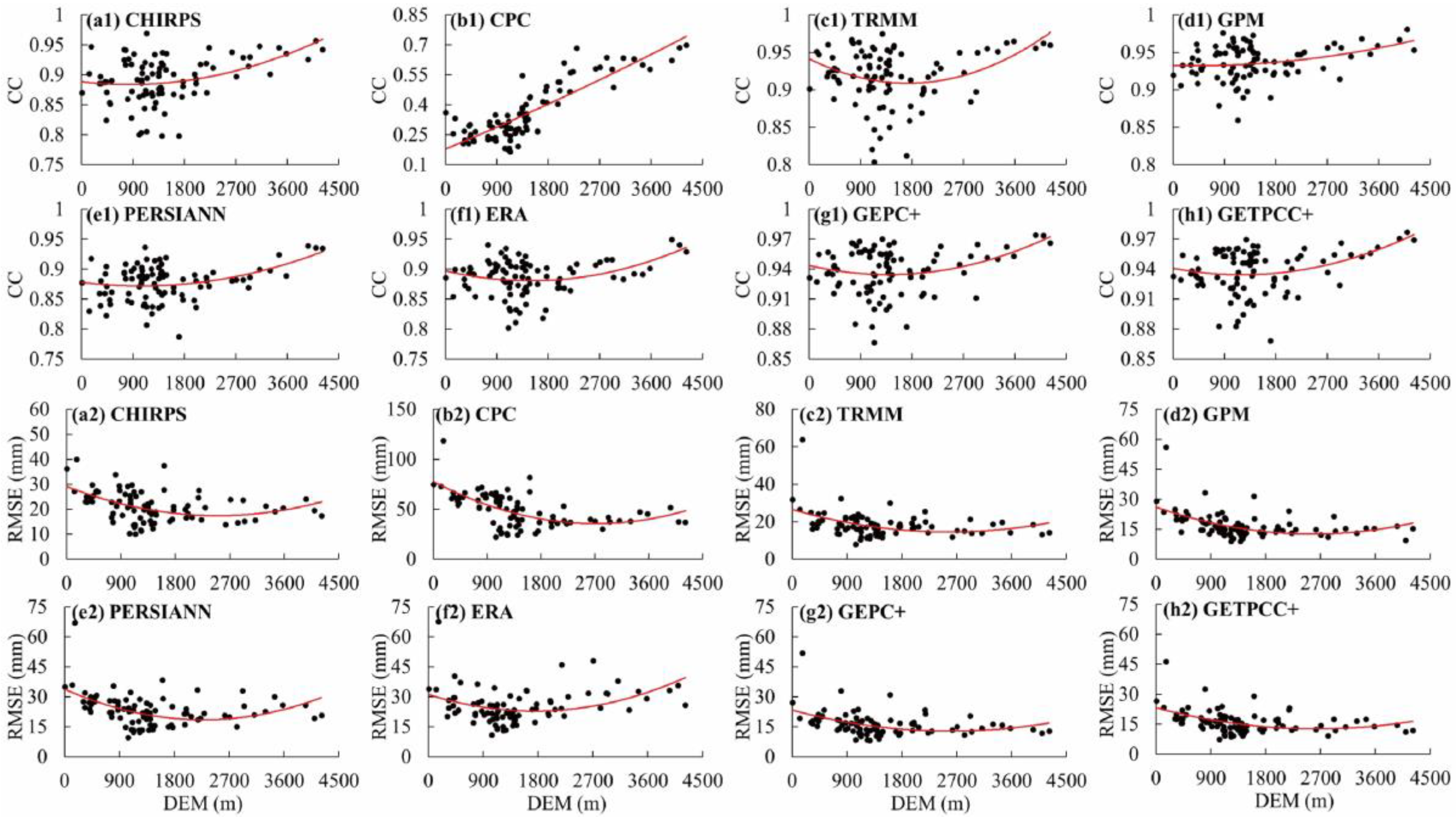
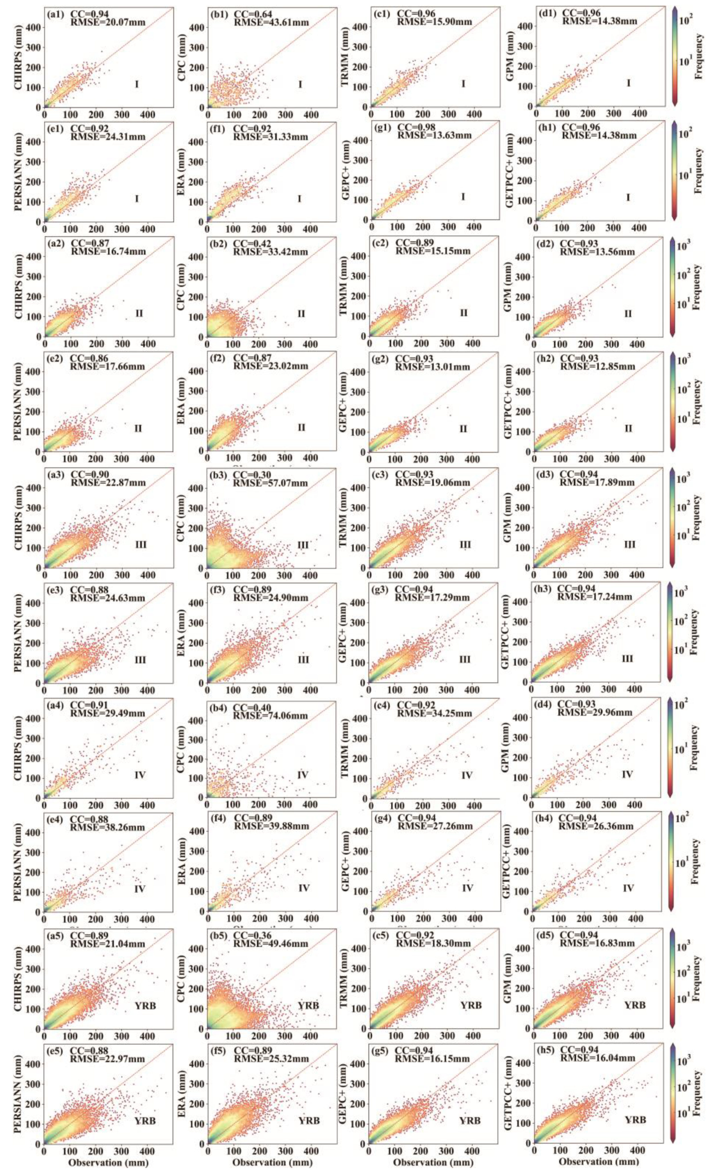
3.2.1. Daily Precipitation Accuracy Evaluation

On a daily scale, quantitative accuracy for precipitation was evaluated using the BIAS, CC, and RMSE at the verification stations. All eight products overestimate the actual precipitation across the YRB, especially the ERA in region IV (

Table 2. Comparison and evaluation of daily observations and simulations. BIAS, CC, RMSE, and DISO are the regional averages of all verification stations.

Statistical Indicators	Products	YRB	Ⅰ	Ⅱ	Ⅲ	Ⅳ
BIAS/%	CHIRPS	9.06	10.37	12.83	6.86	8.83
	CPC	1.81	0.59	6.39	−0.11	−4.9
	TRMM	5.44	1.56	7.56	5.7	−8.51
	GPM	7.38	−2.81	12.69	6.22	−3.24
	PERSIANN	5.82	21.47	6.72	4.5	−3.14
	ERA	25.25	39.19	42.04	15.99	6.47
	GEPC+	7.46	10.31	13.83	3.76	−3.89
	GETPCC+	6.96	9.9	13.03	4.08	−3.4
CC	CHIRPS	0.27	0.28	0.22	0.29	0.28
	CPC	0.05	0.14	0.05	0.03	0.07
	TRMM	0.33	0.33	0.25	0.37	0.3
	GPM	0.42	0.38	0.37	0.46	0.37
	PERSIANN	0.29	0.32	0.24	0.32	0.31
	ERA	0.49	0.49	0.46	0.52	0.46
	GEPC+	0.50	0.50	0.47	0.52	0.45
	GETPCC+	0.46	0.45	0.41	0.5	0.42
RMSE/(mm·d−1)	CHIRPS	6.7	6.14	5.15	7.4	9.54
	CPC	6.12	4.95	4.39	6.99	8.92
	TRMM	5.38	5.1	4.18	5.86	8.03
	GPM	4.99	5.01	3.79	5.46	7.59
	PERSIANN	5.05	5.23	3.78	5.55	7.45
	ERA	4.67	4.07	3.6	5.14	7.09
	GEPC+	4.05	3.55	2.99	4.5	6.5
	GETPCC+	4.39	3.9	3.31	4.84	6.85
DISO	CHIRPS	5.43	3.69	5.98	5.3	5.32
	CPC	5.03	3.02	5.35	5.05	4.96
	TRMM	4.42	3.05	5	4.22	4.53
	GPM	4.06	2.99	4.49	3.91	4.27
	PERSIANN	4.11	3.14	4.49	3.99	4.18
	ERA	3.85	2.48	4.34	3.7	3.97
	GEPC+	3.26	2.06	3.61	3.17	3.49
	GETPCC+	3.58	2.35	3.94	3.47	3.79

). ERA, GEPC+, and GETPCC+ are expected to reveal the highest linear correlation with ground-based observations. The RMSE of ERA, GEPC+, and GETPCC+ is the smallest, with mean values of 4.67 mm, 4.05 mm, and 4.39 mm, respectively. In contrast, CHIRPS and CPC show the highest RMSE with mean values of 6.70 mm and 6.12 mm, respectively. The simulations of multisource integrated precipitation products are closer to the ground-based observations across the YRB relative to SPPs. Meanwhile, the overall performance of GEPC+ (DISO = 3.26) is better than that of GETPCC+ (DISO = 3.58), which confirms that OBMA is very representative in the process of precipitation product integration across the YRB. On the whole, OBIPP (GEPC+) has an overall performance improvement of 9.82% and 18.10% across the YRB relative to BIPP (GETPCC+) and OSPP, respectively, especially in the SRYR by 14.08% and 20.39%. The results reveal that the simulations of GEPC+ across the SRYR are closer to the ground-based observations than other precipitation products.

3.2.2. Precipitation Events Accuracy Evaluation

On a daily scale, quantitative accuracy was evaluated for precipitation events using the POD, FAR, and ETS at the verification stations. It is observed that the POD of eight products across the YRB is enormous differences in the spatial pattern, as shown in Figure 6a. The SRYR shows the highest POD values, while the POD values of MYRB and UYRB are the lowest. Meanwhile, the POD values of different precipitation products are also significant differences. GEPC+ and GETPCC+ exhibit the highest POD values, which are more than 0.96 in most regions, while the POD values of ERA are more than 0.96 only across the SRYR, indicating that ERA and the IPPs have certain advantages in detecting precipitation events.

As shown in Figure 6b, the spatial distribution pattern of FAR across the YRB is similar to that of POD, and there are low FAR values across the SRYR. ERA exhibit the lowest FAR values, followed by GPM and TRMM, while CPC exhibits the highest FAR values. All eight products demonstrate that the FAR values are lowest across the SRYR, which range from 0.36 to 0.61. The results reveal that the IPPs across the YRB are prone to false alarms about precipitation events compared with SPPs.

The ETS of all eight products is lower than 0.35 (Figure 6c). GEPC+ exhibits the highest ETS with an average value of 0.26, followed by GETPCC+ and ERA. CHIRPS, CPC, and PERSIANN-CDR exhibit similar ETS. The average values are less than 0.13. Overall, the precipitation event capture capacity of OBIPP (GEPC+) across the YRB increased by 4.39% and 6.98% relative to BIPP (GETPCC+) and OSPP, respectively, especially in the SRYR by 7.50% and 37.93%. The results reveal that GEPC+ across the SRYR has tremendous advantages in detecting precipitation events.

3.2.3. Monthly Scale Accuracy Evaluation

Firstly, we evaluated the dependence of monthly precipitation products on altitude (Figure 7). It can be observed from Figure 7(a1–h1) that the CC values of the CPC show an obvious upward trend with the increase in altitude. In contrast, CC values of the other products offer a slight change trend, indicating that the agreement between simulations and observations of CPC is more dependent on altitude than other products. All eight products with an elevation between 900 and 1800 m have the lowest RMSE. The RMSE values of the TRMM, GPM, GEPC+, and GETPCC+ offer the slightest change, indicating that the error magnitude of these four products is less dependent on elevation (Figure 7(a2–h2)).

To further verify the performance of the OBIPP at the monthly scale, we exploited the monthly precipitation of the verification stations to quantify the associated algorithm uncertainties. Figure 8a–h, respectively, display the scatter plots of monthly precipitation estimates from the eight products versus the monthly precipitation of verification stations. GEPC+ across the SRYR exhibit excellent performance, while GETPCC+ across the other regions reveals good performance with the lowest RMSE and highest CC. CPC exhibits the highest RMSE and the lowest CC with mean values of 49.46 mm and 0.36, respectively, and in particular, the RMSE and CC of CPC are 57.07 mm and 0.30 across the MYRB. GEPC+ can represent the monthly precipitation features across the SRYR, GETPCC+ can reflect the monthly precipitation features for other regions, and CPC cannot reflect the monthly precipitation features of the YRB.

3.3. Hydrological Assessment of Multisource Integrated Precipitation Products

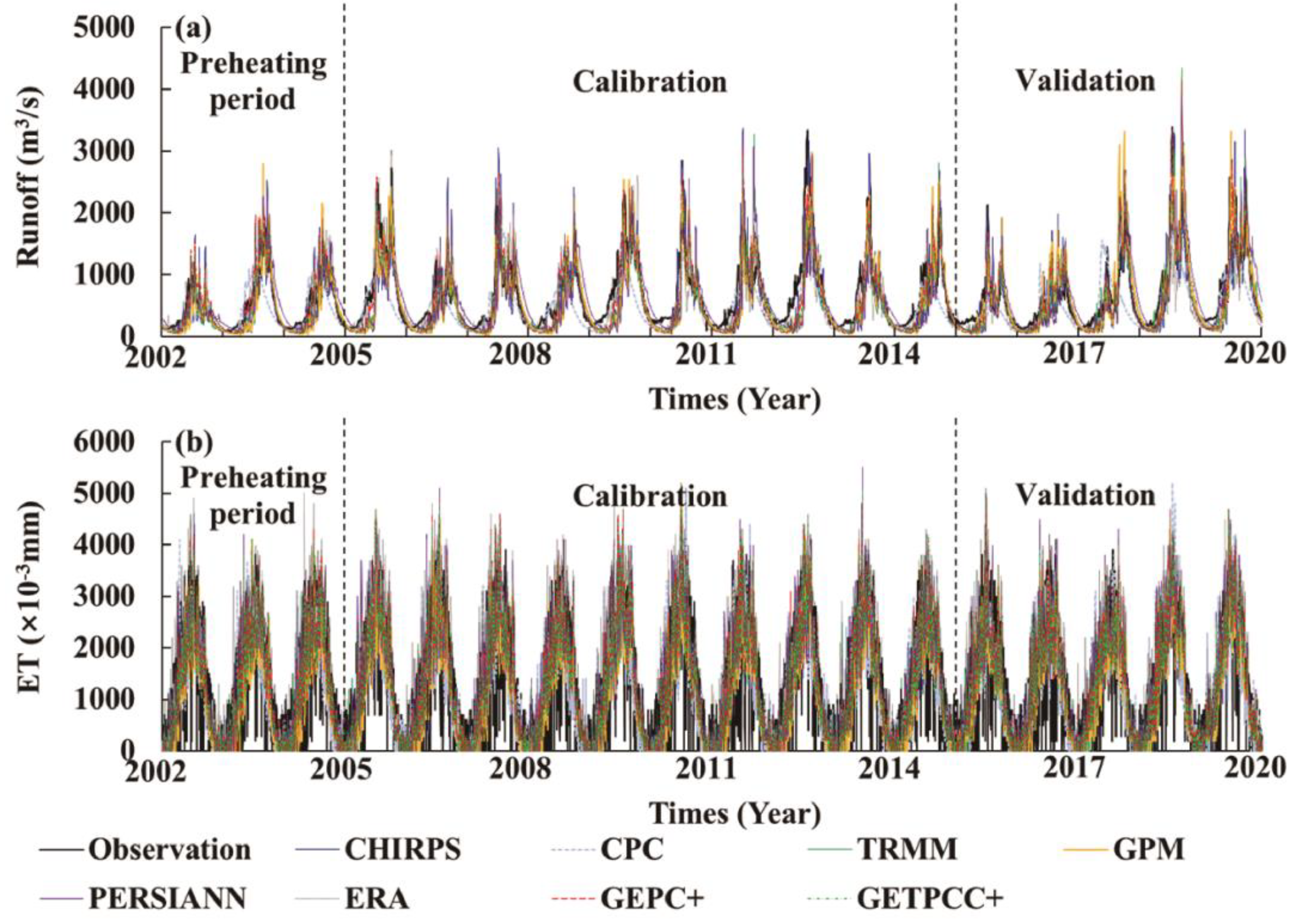
3.3.1. Simulation of Daily Runoff and Evapotranspiration

To further explore the simulation accuracy of the IPPs, our study reveals the simulation performance of eight products for runoff and evapotranspiration. The performance of the VIC model driven by eight products for the TNH station is shown in Figure 8 and

Table 3. Evaluation of VIC simulated runoff and evapotranspiration drove by eight precipitation products.

Station	Products	Preheating Period (2002–2005)			Calibration (2006–2015)			Validation (2016–2019)
		NSE	CC	BIAS (%)	NSE	CC	BIAS (%)	NSE	CC	BIAS (%)
TNH (Daily runoff)	CHIRPS	0.62	0.83	−15.86	0.60	0.83	−14.38	0.64	0.84	−13.77
	CPC	0.39	0.69	−26.31	0.44	0.78	−32.46	0.40	0.71	−27.48
	TRMM	0.71	0.87	−18.57	0.57	0.81	−21.94	0.70	0.86	−5.81
	GPM	0.69	0.87	−15.17	0.60	0.83	−19.55	0.69	0.88	−2.87
	PERSIANN	0.64	0.82	0.73	0.38	0.69	−14.24	0.63	0.83	0.04
	ERA5	0.80	0.94	11.84	0.68	0.85	−13.95	0.61	0.84	−25.20
	GEPC+	0.76	0.90	2.40	0.74	0.89	−11.10	0.81	0.92	−8.45
	GETPCC+	0.76	0.89	−6.53	0.69	0.87	−16.43	0.74	0.88	−14.05
TNH (Daily ET)	CHIRPS	0.59	0.78	−11.55	0.54	0.76	−9.28	0.53	0.76	−6.13
	CPC	0.48	0.73	−14.84	0.42	0.70	−12.22	0.42	0.70	−7.78
	TRMM	0.58	0.79	−16.68	0.58	0.78	−12.79	0.57	0.77	−8.70
	GPM	0.58	0.81	−23.08	0.57	0.79	−19.30	0.61	0.80	−12.56
	PERSIANN	0.57	0.78	1.56	0.53	0.76	3.43	0.52	0.77	11.37
	ERA5	0.42	0.82	34.43	0.37	0.79	33.64	0.35	0.79	30.27
	GEPC+	0.63	0.81	−4.82	0.61	0.80	−3.96	0.61	0.80	1.69
	GETPCC+	0.62	0.80	−7.17	0.60	0.79	−5.96	0.60	0.79	−0.47

. The simulated runoff of eight precipitation products agrees with the observations, and all products capture the dynamic changes and flood peak scenarios similar to the observations (Figure 9a). However, GEPC+ across the SRYR exhibit excellent performance for hydrological simulation. During calibration and verification periods of GEPC+, NSE is 0.74 and 0.81, CC is 0.89 and 0.92, and BIAS is −11.10% and −8.45%, respectively (Table 3). Meanwhile, our research confirms that the simulated runoff by all eight precipitation products overestimates the observations, especially in the non-rainy season. It can be seen from the NSE in the validation period that OBIPP (GEPC+) has the runoff simulation performance improvement of 9.46% and 15.71% across the SRYR relative to BIPP (GETPCC+) and OSPP, respectively.

The simulated evapotranspiration of eight precipitation products agrees with the observations, and all products capture the seasonal dynamic changes similar to the observations (Figure 9b). All eight products overestimate evapotranspiration in the rainy season across the SRYB, while GEPC+ still has the highest simulation performance for evapotranspiration (NSE > 0.6, CC > 0.8, BIAS < 5%). Based on the ERA5-LAND evapotranspiration product, our research verifies the reliability of simulated evapotranspiration using GEPC+ for the spatial pattern (Figure 10). The simulated results have consistent spatial distribution and temporal dynamics with the ERA5-LAND evapotranspiration product. Meanwhile, the multiyear average simulated results are overestimated relative to the ERA5-LAND evapotranspiration product (BIAS = 3.54%), and BIAS of the non-rainy season is more significant across the southeastern of the SRYR, with the BIAS higher than 20%. Considering the uncertainty of the ERA5-LAND evapotranspiration product, our research believes that the overall simulation results show high reliability.

3.3.2. Uncertainty Analysis

The uncertainty of spatial and temporal distribution of precipitation across the SRYR is crucial for runoff simulation. Figure 11a shows the annual mean precipitation values distribution from OBIPP. Annual mean precipitation shows a spatial pattern increasing from northwest to southeast. In the southeastern region, the mean precipitation is higher than 800 mm, while the mean precipitation in the northwestern region is lower than 400 mm. Figure 11b shows the precipitation uncertainty across the SRYR by the coefficient of variation. The coefficient of variation value is about 11%, and the precipitation variation is mainly concentrated in the northeast, where the coefficient of variation is above 13%. During 2001–2019 (Figure 11c,d), the average precipitation across the SRYR was about 621 mm, with fluctuation intervals (95% confidence intervals) ranging from 341 to 900 mm. It shows an overall trend of significant increase (5.15 mm/a). In addition, the precipitation across the SRYR has noticeable seasonal differences, with most of the precipitation concentrated in summer, and the average precipitation from May to September is higher than 100 mm/month, while the average precipitation from October to April is lower than 18 mm/month (Figure 11e).

Figure 12a shows the spatial distribution, uncertainty, and change trend of runoff simulated by OBIPP across the SRYR. The annual average runoff depth across the SRYR presents a spatial distribution similar to precipitation, showing an increasing spatial pattern from northwest to southeast, from more than 160 mm to less than 40 mm. The uncertainty of runoff depth is mainly concentrated in the northwest of the SRYR, with a variation coefficient of more than 20% (Figure 12b). During 2001–2019, the average runoff depth across the SRYR was 63.50 mm, with a fluctuation interval (95% confidence interval) of 42–84 mm; The runoff depth generally shows an increasing trend, about 0.71 mm/a, while the runoff depth in the southeast increases with a trend of more than 1.6 mm/a (Figure 12c,d). The runoff depth across the SRYR is similar to the precipitation, with noticeable seasonal differences. The high value of runoff depth is concentrated in summer. The average runoff depth from May to September is higher than 11 mm/month, while the average runoff depth from October to April is lower than 2 mm/month (Figure 12e).

4. Discussion

An enormous amount of research has achieved consensus that SPPs are likely to be insufficient for accurate precipitation monitoring [19,49]. However, previous research ignored that poor regional simulation of a particular forecast member can affect the overall forecast results [10,11]. In this research, the OBIPP was developed based on the OBMA to calculate the assigned weights for the inputs SPPs of different combinations and screen the optimal multisource integrated precipitation product on multitemporal scales to reflect the precipitation information. To test the sensitivity of OBIPP to precipitation monitoring, the ground-based observations of verification stations were utilized. The results show that the detecting accuracy of the same precipitation product in different subregions has obvious regional heterogeneity. However, CC is the largest in different sub-regions, which does not mean that RMSE is the smallest. The main reason is that CC can only reflect the consistency of the data of two groups and cannot reflect the difference in values between them. The RMSE values are related to the spatial distribution of precipitation across the YRB, and the greater the magnitude of precipitation, the greater the regional RMSE.

Meanwhile, our research reveals that all eight products overestimate actual precipitation relative to ground-based observations, especially ERA5. Previous works have confirmed that SSPs such as PERSIANN, GPM, and ERA5 overestimate actual precipitation in almost all cases [50,51,52], and some related studies have shown that ERA5 is reliable for precipitation information across the YRB but has some limitations in detecting precipitation events [49]. OBIPP improved by 18.10% and 9.82% in overall performance relative to BIPP and ERA across the YRB, respectively (Table 2). We also confirmed that ERA5 and integrated products are superior to other satellite precipitation products in correctly detecting precipitation events, which are prone to omit weak precipitation events, and ice and snow cover has a strong interference effect on reflected signals, leading to a weakening of the detection ability of snow events [53]. The IPPs still have some disadvantages. The FAR values of OBIPP are higher, but the precipitation event capture capacity is still improved by 37.93% relative to OSPP.

This study also found that the CC between the simulations and observations of all eight products decreased sharply as the time scale decreased from monthly to daily, with CC values of the OBIPP dropping from 0.94 to 0.50, indicating that OBIPP is inferior to the monthly precipitation in capturing the daily precipitation dynamics across the YRB. With the elevation increase, the RMSE values of TRMM, GPM, BIPP, and OBIPP are the most stable products, indicating that the error magnitude of these four precipitation products is less dependent on elevation. Based on the above analysis, BIPP can generally provide more accurate daily and monthly precipitation information across the YRB than other products. Our research structures the BMA based on the observations of 222 calibration stations and utilizes the observations of 90 verification stations as the evaluation benchmark to finally screen out OBIPP. However, the terrain of the YRB fluctuates wildly, and the meteorological conditions are complex. Using the precipitation records of the limited number of ground-based observation stations to structure the model will still produce errors. Therefore, the results of precipitation assessment across the YRB should be treated with caution.

Meanwhile, to obtain the spatial weight of BMA more directly, we mapped the spatial weight using inverse distance-weighted (IDW) interpolation. The advantage of IDW is that it is easy to understand and operate, while the disadvantage of IDW is it only considering the distance between the known sample point and the point to be interpolated without considering the influence of other factors and the change rule, such as landform parameters, atmospheric parameters, etc. However, several alternative interpolation methods can reduce the impact of terrain and atmosphere on interpolation, such as the Anuspline method and synchronous mapping system (SYMAP) algorithm [32,54]. Therefore, in future research, multiple interpolation methods should be considered to reduce the impact of terrain and atmospheric parameters on BMA weight.

In the SRYR, precipitation information of OBIPP is superior to other products, and the available ground-based stations are relatively sparse (Figure 1, 1 < /104 km²). Therefore, we choose SRYR to evaluate the applicability of OBIPP in hydrological simulation to prove that OBIPP can fill the gap in precipitation information. Previous studies have shown that GPM is superior to TRMM in daily and sub-daily runoff simulation, while APHRODITE and TRMM are more representative than CPC, CN05.1, PERSIANN-CDR, and Princeton Global Forcing in monthly runoff simulation [19,55]. In addition, numerous studies have evaluated the applicability of the VIC model driven by multisource precipitation products in different basins around the world [56,57,58]. The VIC model is a large-scale hydrological model with variable infiltration capacity that solves each grid cell’s hydrologic and energy balance [59]. Unlike previous studies, the VIC model driven by OBIPP can better simulate the daily runoff of the SRYR in a long time series relative to other precipitation products. This study confirms that OBIPP has more substantial hydrological application potential. For example, flood simulation and early warning are carried out in remote regions with sparse ground-based stations.

Moreover, LUCC has an essential impact on the regional hydrological cycle. Many studies have confirmed that the increase in grassland and forest land cause a decreasing trend in runoff, while the increase in cultivated land and impervious surfaces leads to an increase in runoff [60,61]. The runoff change in the SRYR is mainly affected by climate change but little by LUCC [62]. Therefore, the selection of LUCC has little impact on runoff simulation in the SRYR. However, selecting only LUCC from a single source for large-scale regional studies will increase the uncertainty of hydrological simulation. LUCC from multiple sources should be considered to reduce the uncertainty of runoff simulation, such as the MYRB.

5. Conclusions

In this work, six SPPs, BIPP, and OBIPP were evaluated at daily and monthly scales from 2001 to 2019 across the YRB. Based on the VIC model, the applicability of eight products in the hydrological simulation of the SRYR is discussed. The main findings are as follows.

(1)

OBIPP (GEPC+) is remarkably correlated with ground-based observations and displays the lowest RMSE and highest CC at the daily scales. OBIPP across the SRYR exhibited excellent performance at the monthly scales, while BIPP (GETPCC+) across the other regions revealed good performance.

(2)

OBIPP and BIPP exhibited the highest POD values for the detection accuracy of precipitation events. ERA and CPC exhibit the lowest and highest FAR values, respectively. OBIPP exhibited the highest ETS, followed by GETPCC+ and ERA.

(3)

The VIC model driven by daily OBIPP with a Nash coefficient (NSE) of runoff simulation for both calibration and validation periods exceeds 0.74 and 0.81, respectively. The simulated runoff and evapotranspiration of the VIC model driven by daily OBIPP exhibit the highest CC and NSE during the validation periods. Overall, the daily precipitation corrected by the OBMA can meet the application requirements of hydrological simulation.

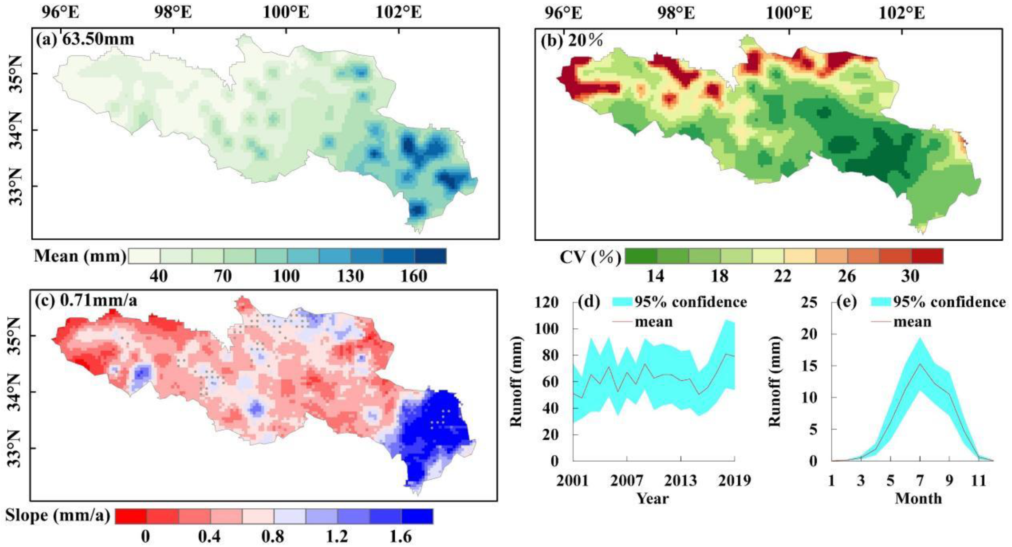
(4)

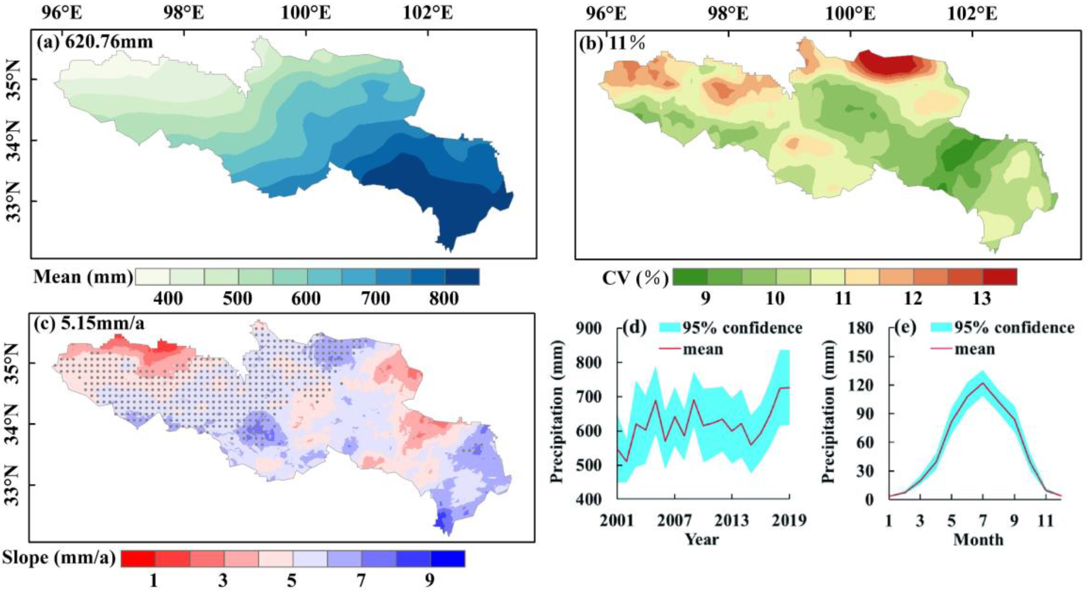
OBIPP simulation results show that the average annual precipitation and runoff depth across the SRYR was 621 mm and 63.50 mm from 2001 to 2019, respectively, showing the spatial pattern of increasing from northwest to southeast. The interannual variations of annual precipitation and runoff depth have a significantly increasing trend. They all show a more significant uncertainty in the northwest region.

The spatial and daily variations among the eight precipitation products impact the performance of hydrological simulations. Our work’s integrated product can provide a fundamental approach for the optimal selection of single precipitation products for driving hydrological models or other hydroclimatological-related tasks across the YRB. Further, this work aims to improve the accuracy of precipitation monitoring by developing a multisource integrated precipitation product that can be applied across the YRB and doesn’t depend on data from ground-based observations. The quantified precipitation variability for integrated products will help characterize sources of uncertainty for hydro-climatological analyses in similar regions or basins. Additionally, this study provides research insights for the development of multisource integrated precipitation products to improve runoff simulation and forecasting in areas with no or little precipitation data. Meanwhile, it should be noted that the snow cover across the SRYR still needs to be made available. The snow cover module is the default parameter, which may be the main reason for underestimating the non-rainy season runoff. Future work should involve obtaining snow module parameters for various spatial–temporal scales using remote sensing satellite products.

References

1. Li, Y.Y.; Cao, J.T.; Huang, H.J.; Xing, Z.Q. International progresses in integrated water resources management. Adv. Water Sci. 2018, 29, 127–137. [Google Scholar] [CrossRef]
2. Miller, J.D.; Kim, H.; Kjeldsen, T.R.; Packman, J.; Grebby, S.; Dearden, R. Assessing the impact of urbanization on storm runoff in a peri-urban catchment using historical change in impervious cover. J. Hydrol. 2014, 515, 59–70. [Google Scholar] [CrossRef] [Green Version]
3. Wang, X.; Chen, D.; Pang, G.; Gou, X.; Yang, M. Historical and future climates over the upper and middle reaches of the Yellow River Basin simulated by a regional climate model in CORDEX. Clim. Dyn. 2021, 56, 2749–2771. [Google Scholar] [CrossRef]
4. Fries, A.; Rollenbeck, R.; Bayer, F.; Gonzalez, V.; Oñate-Valivieso, F.; Peters, T.; Bendix, J. Catchment precipitation processes in the San Francisco valley in southern Ecuador: Combined approach using high-resolution radar images and in situ observations. Meteorol. Atmos. Phys. 2014, 126, 13–29. [Google Scholar] [CrossRef]
5. Hao, Z.C.; Tong, K.; Zhang, L.L.; Duan, X.L. Applicability Analysis of TRMM Precipitation Estimates in Tibetan Plateau. J. China Hydrol. 2011, 31, 18–23. (In Chinese) [Google Scholar]
6. Ma, Z.; Sun, P.; Zhang, Q.; Zou, Y.; Lv, Y.; Li, H.; Chen, D. The Characteristics and Evaluation of Future Droughts across China through the CMIP6 Multi-Model Ensemble. Remote Sens. 2022, 14, 1097. [Google Scholar] [CrossRef]
7. Shen, Y.; Xiong, A.; Hong, Y.; Yu, J.; Pan, Y.; Chen, Z.; Saharia, M. Uncertainty analysis of five satellite-based precipitation products and evaluation of three optimally merged multi-algorithm products over the Tibetan Plateau. Int. J. Remote Sens. 2014, 35, 6843–6858. [Google Scholar] [CrossRef]
8. Chao, L.; Zhang, K.; Li, Z.; Zhu, Y.; Wang, J.; Yu, Z. Geographically Weighted Regression Based Methods for Merging Satellite and Gauge Precipitation. J. Hydrol. 2018, 558, 275–289. [Google Scholar] [CrossRef]
9. Chen, F.; Gao, Y.; Wang, Y.; Li, X. A Downscaling-Merging Method for High-Resolution Daily Precipitation Estimation. J. Hydrol. 2020, 581, 124414. [Google Scholar] [CrossRef]
10. Sun, R.; Yuan, H.; Yang, Y. Using Multiple Satellite-gauge Merged Precipitation Products Ensemble for Hydrologic Uncertainty Analysis over the Huaihe River Basin. J. Hydrol. 2018, 566, 406–420. [Google Scholar] [CrossRef] [Green Version]
11. Rahman, K.U.; Shang, S.; Shahid, M.; Wen, Y.; Khan, Z. Application of Dynamic Clustered Bayesian Model Averaging (DCBA) Algorithm for Merging Multi-Satellite Precipitation Products over Pakistan. J. Hydrometeorol. 2020, 21, 17–37. [Google Scholar] [CrossRef]
12. Lu, X.; Wei, M.; Tang, G.; Zhang, Y. Evaluation and correction of the TRMM 3B43V7 and GPM 3IMERGM satellite precipitation products by use of ground-based data over Xinjiang, China. Environ. Earth Sci. 2018, 77, 209. [Google Scholar] [CrossRef]
13. Zhou, L.; Koike, T.; Takeuchi, K.; Rasmy, M.; Onuma, K.; Ito, H.; Selvarajah, H.; Liu, L.; Li, X.; Ao, T. A study on availability of ground observations and its impacts on bias correction of satellite precipitation products and hydrologic simulation efficiency. J. Hydrol. 2022, 610, 127595. [Google Scholar] [CrossRef]
14. Duan, Z.; Ren, Y.; Liu, X.; Lei, H.; Hua, X.; Shu, X.; Zhou, L. A comprehensive comparison of data fusion approaches to multi-source precipitation observations: A case study in Sichuan province, China. Environ. Monit. Assess. 2022, 194, 422. [Google Scholar] [CrossRef]
15. Pan, Y.; Yuan, Q.; Ma, J.; Wang, L. Improved Daily Spatial Precipitation Estimation by Merging Multi-Source Precipitation Data Based on the Geographically Weighted Regression Method: A Case Study of Taihu Lake Basin, China. Int. J. Environ. Res. Public Health 2022, 19, 13866. [Google Scholar] [CrossRef]
16. Lin, M.; Biswas, A.; Bennett, E.M. Spatio-temporal dynamics of groundwater storage changes in the Yellow River Basin. J. Environ. Manag. 2019, 235, 84–95. [Google Scholar] [CrossRef]
17. Zhou, D.; Zhang, B.; An, M.L.; Zhang, Y.; Li, J. Responses of drought with different time scales to the ENSO events in the Yellow River Basin. J. Desert Res. 2015, 35, 753–762. (In Chinese) [Google Scholar]
18. Peng, Y.; Zhao, X.; Wu, D.; Tang, B.; Xu, P.; Du, X.; Wang, H. Spatiotemporal Variability in Extreme Precipitation in China from Observations and Projections. Water 2018, 10, 1089. [Google Scholar] [CrossRef] [Green Version]
19. Guan, X.; Zhang, J.; Yang, Q.; Tang, X.; Liu, C.; Jin, J.; Liu, Y.; Bao, Z.; Wang, G. Evaluation of Precipitation Products by Using Multiple Hydrological Models over the Upper Yellow River Basin, China. Remote Sens. 2020, 12, 4023. [Google Scholar] [CrossRef]
20. Shi, J.; Yuan, F.; Shi, C.; Zhao, C.; Zhang, L.; Ren, L.; Zhu, Y.; Jiang, S.; Liu, Y. Statistical Evaluation of the Latest GPM-Era IMERG and GSMaP Satellite Precipitation Products in the Yellow River Source Region. Water 2020, 12, 1006. [Google Scholar] [CrossRef] [Green Version]
21. Gu, P.; Wang, G.; Liu, G.; Wu, Y.; Liu, H.; Jiang, X.; Liu, T. Evaluation of multisource precipitation input for hydrological modeling in an Alpine basin: A case study from the Yellow River Source Region. Hydrol. Res. 2022, 53, 314–335. [Google Scholar] [CrossRef]
22. Gao, T.; Wang, H. Trends in precipitation extremes over the Yellow River basin in North China: Changing properties and causes. Hydrolgical Process. 2017, 31, 2412–2428. [Google Scholar] [CrossRef]
23. Shen, Y.; Xiong, A. Validation and comparison of a new gauge-based precipitation analysis over mainland China. Int. J. Climatol. 2016, 36, 252–265. [Google Scholar] [CrossRef]
24. Funk, C.; Peterson, P.; Landsfeld, M.; Pedreros, D.; Verdin, J.; Shukla, S.; Husak, G.; Rowland, J.; Harrison, L.; Hoell, A.; et al. The climate hazards infrared precipitation with stations—A new environmental record for monitoring extremes. Sci. Data 2015, 2, 150066. [Google Scholar] [CrossRef] [PubMed] [Green Version]
25. Xie, P.; Yatagai, A.; Chen, M.; Yang, S.; Yatagai, A.; Hayasaka, T.; Fukushima, Y.; Liu, C. A gauge based analysis of daily precipitation over East Asia. J. Hydrometeorol. 2007, 8, 607–626. [Google Scholar] [CrossRef]
26. Huffman, G.J. Estimates of Root-Mean-Square Random Error for Finite Samples of Estimated Precipitation. J. Appl. Meteorol. Climatol. 1997, 36, 1191–1201. [Google Scholar] [CrossRef]
27. Huffman, G.J.; Bolvin, D.T.; Braithwaite, D.; Hsu, K.; Joyce, R.; Kidd, C.; Nelkin, E.J.; Sorooshian, S.; Jackson, T.; Xie, P. Algorithm Theoretical Basis Document (ATBD) Version 4.4 for the NASA Global Precipitation Measurement(GPM) Integrated Multi-satellite Retrievals for GPM (IMERG); NASA/GSFC Code: Greenbelt, MD, USA, 2014; Volume 612, pp. 1–26. [Google Scholar]
28. Ashouri, H.; Hsu, K.; Sorooshian, S.; Braithwaite, D.K.; Knapp, K.R.; Cecil, L.D.; Nelson, B.R.; Prat, O.P. PERSIANN CDR: Daily precipitation climate data record from multi-satellite observations for hydrological and climate studies. Bull. Am. Meteorol. Soc. 2015, 96, 69–83. [Google Scholar] [CrossRef] [Green Version]
29. Hersbach, H.; Bell, B.; Berrisford, P.; Hirahara, S.; Horányi, A.; Muñoz-Sabater, J.; Nicolas, J.; Peubey, C.; Radu, R.; Schepers, D.; et al. The ERA5 global reanalysis. Q. J. R. Meteorol. Soc. 2020, 146, 1999–2049. [Google Scholar] [CrossRef]
30. Nijssen, B.; Schnur, R.; Lettenmaier, D.P. Global retrospective estimation of soil moisture using the variable infiltration capacity land surface model,1980–93. J. Clim. 2001, 14, 1790–1808. [Google Scholar] [CrossRef]
31. Wei, S.; Dai, Y.; Liu, B.; Zhu, A.; Duan, Q.; Wu, L.; Ji, D.; Ye, A.; Yuan, H.; Zhang, Q.; et al. A China data set of soil properties for land surface modeling. J. Adv. Model. Earth Syst. 2013, 5, 212–224. [Google Scholar] [CrossRef]
32. Zhu, B.; Xie, X.; Lu, C.; Lei, T.; Wang, Y.; Jia, K.; Yao, Y. Extensive evaluation of a continental-scale high-resolution hydrological model using remote sensing and ground based observations. Remote Sens. 2021, 13, 1247. [Google Scholar] [CrossRef]
33. Liu, Y.; Yang, Z.; Lin, P.; Zheng, Z.; Xie, S. Comparison and evaluation of multiple land surface products for the water budget in the Yellow River Basin. J. Hydrol. 2019, 584, 124534. [Google Scholar] [CrossRef]
34. Raftery, A.E.; Gneiting, T.; Balabdaoui, F.; Polakowski, M. Using Bayesian Model Averaging to Calibrate Forecast Ensembles. Mon. Weather. Rev. 2005, 133, 1155–1174. [Google Scholar] [CrossRef] [Green Version]
35. Dong, L.H.; Xiong, L.H.; Wan, M. Uncertainty analysis of hydrological modeling using the Bayesian Model Averaging Method. J. Hydraul. Eng. 2001, 42, 1065–1074. (In Chinese) [Google Scholar]
36. Hu, Z.; Chen, X.; Zhou, Q.; Chen, D.; Li, J. DISO: A rethink of Taylor diagram. Int. J. Climatol. 2019, 39, 2825–2832. [Google Scholar] [CrossRef]
37. Cherkauer, K.A.; Lettenmaier, D.P. Hydrologic effects of frozen soils in the upper Mississippi River basin. J. Geophys. Res. Atmos. 1999, 104, 19599–19610. [Google Scholar] [CrossRef]
38. Liang, X.; Lettenmaie, D.P.; Wood, E.F.; Burges, S.J. A simple hydrologically based model of land-surface water and energy fluxes. J. Geophys. Res. Atmos. 1994, 99, 14415–14428. [Google Scholar] [CrossRef]
39. Liang, X.; Lettenmaie, D.P.; Wood, E.F. One-dimensional statistical dynamic representation of subgrid spatial variability of precipitation in the two-layer variable infiltration capacity model. J. Geophys. Res. Atmos. 1996, 101, 21403–21422. [Google Scholar] [CrossRef]
40. Wilks, D. Statistical Methods in the Atmospheric Sciences. Technom 2006, 102, 380. [Google Scholar]
41. Mashingia, F.; Mtalo, F.; Bruen, M. Validation of remotely sensed rainfall over major climatic regions in Northeast Tanzania. Phys. Chem. Earth Parts A/B/C 2014, 67, 55–63. [Google Scholar] [CrossRef]
42. Budyko, M.I. Climate and Life; Academic Press: New York, NY, USA, 1974; p. 508. [Google Scholar]
43. Penman, H.L. Natural evaporation from open water, hare soil and grass. Proc. R. Soc. A Math. Phys. Eng. Sci. 1948, 193, 120–145. [Google Scholar] [CrossRef] [Green Version]
44. Choudhury, B.J. Evaluation of an empirical equation for annual evaporation using field observations and results from a biophysical model. J. Hydrol. 1999, 216, 99–110. [Google Scholar] [CrossRef]
45. Yang, H.B.; Yang, D.W.; Lei, Z.D.; Sun, F.B. New analytical derivation of the mean annual water-energy balance equation. Water Resour. Res. 2008, 44, W03410. [Google Scholar] [CrossRef]
46. Xu, X.Y.; Yang, D.W.; Yang, H.B.; Lei, H.M. Attribution analysis based on the Budyko hypothesis for detecting the dominant cause of runoff decline in Haihe basin. J. Hydrol. 2014, 510, 530–540. [Google Scholar] [CrossRef]
47. Yang, H.B.; Qi, J.; Xu, X.Y.; Yang, D.W.; Lv, H.F. The regional variation in climate elasticity and climate contribution to runoff across China. J. Hydrol. 2014, 517, 607–616. [Google Scholar] [CrossRef]
48. Ning, T.T.; Li, Z.; Liu, W.Z. Separating the impacts of climate change and land surface alteration on runoff reduction in the Jing River catchment of China. Catena 2016, 147, 80–86. [Google Scholar] [CrossRef]
49. An, Y.; Zhao, W.; Li, C.; Liu, Y. Evaluation of Six Satellite and Reanalysis Precipitation Products Using Gauge Observations over the Yellow River Basin, China. Atmosphere 2020, 11, 1223. [Google Scholar] [CrossRef]
50. Yang, Y.; Luo, Y. Evaluating the performance of remote sensing precipitation products CMORPH, PERSIANN, and TMPA, in the arid region of northwest China. Theor. Appl. Climatol. 2014, 118, 429–445. [Google Scholar] [CrossRef]
51. Jiang, Q.; Li, W.; Fan, Z.; He, X.; Sun, W.; Chen, S.; Wen, J.; Gao, J.; Wang, J. Evaluation of the ERA5 reanalysis precipitation dataset over Chinese Mainland. J. Hydrol. 2021, 595, 125660. [Google Scholar] [CrossRef]
52. Zhu, H.; Chen, S.; Li, Z.; Gao, L.; Li, X. Comparison of Satellite Precipitation Products: IMERG and GSMaP with Rain Gauge Observations in Northern China. Remote Sens. 2022, 14, 4748. [Google Scholar] [CrossRef]
53. Scheel, M.; Rohrer, M.; Huggel, C.; Villar, D.S.; Silvestre, E.; Huffman, G.J. Evaluation of TRMM multi-satellite precipitation analysis (TMPA) performance in the Central Andes region and its dependency on spatial and temporal resolution. Hydrol. Earth Syst. Sci. 2011, 15, 2649–2663. [Google Scholar] [CrossRef] [Green Version]
54. Ren, Y.; Liu, J.; Liu, S.; Wang, Z.; Liu, T.; Shalamzari, M.J. Effects of Climate Change on Vegetation Growth in the YellowRiver Basin from 2000 to 2019. Remote Sens. 2022, 14, 687. [Google Scholar] [CrossRef]
55. Yuan, F.; Wang, B.; Shi, C.; Cui, W.; Zhao, C.; Liu, Y.; Ren, L.; Zhang, L.; Zhu, Y.; Chen, T.; et al. Evaluation of hydrological utility of IMERG Final run V05 and TMPA 3B42V7 satellite precipitation products in the Yellow River source region, China. J. Hydrol. 2018, 567, 696–711. [Google Scholar] [CrossRef]
56. Tong, K.; Su, F.; Yang, D.; Hao, Z. Evaluation of satellite precipitation retrievals and their potential utilities in hydrologic modeling over the Tibetan Plateau. J. Hydrol. 2014, 519, 423–437. [Google Scholar] [CrossRef]
57. Huang, Y.H.; Zhang, Z.X.; Fei, M.Z.; Jin, Q. Hydrological evaluation of the TMPA multisatellite precipitation estimates over the Gangjiang basin. Resour. Environ. Yangtze Basin 2016, 10, 1618–1625. (In Chinese) [Google Scholar]
58. Zhu, B.; Huang, Y.; Zhang, Z.; Kong, R.; Tian, J.; Zhou, Y.; Chen, S.; Duan, Z. Evaluation of TMPA Satellite Precipitation in Driving VIC Hydrological Model over the Upper Yangtze River Basin. Water 2020, 12, 3230. [Google Scholar] [CrossRef]
59. Xu, L. A Two-Layer Variable Infiltration Capacity Land Surface Representation for General Circulation Models. Ph.D. Thesis, University of Washington, Washington, DC, USA, 1 May 1994. [Google Scholar]
60. Gebremicael, T.G.; Mohamed, Y.A.; Betrie, G.D.; Zaag, P.; Teferi, E. Trend analysis of runoff and sediment fluxes in the Upper Blue Nile basin: A combined analysis of statistical tests, physically-based models and landuse maps. J. Hydrol. 2013, 482, 57–68. [Google Scholar] [CrossRef]
61. Nosetto, M.D.; Jobbágy, E.G.; Paruelo, J.M. Land-use change and water losses: The case of grassland afforestation across a soil textural gradient in central Argentina. Glob. Change Biol. 2010, 11, 1101–1117. [Google Scholar] [CrossRef]
62. Ni, Y.; Yu, Z.; Lv, X.; Qing, T.; Yan, D.; Zhang, Q.; Ma, L. Spatial difference analysis of the runoff evolution attribution in the Yellow River Basin. J. Hydrol. 2022, 612, 128149. [Google Scholar] [CrossRef]
Figure 1. (a) The geographical location of the Yellow River Basin in China; (b) digital elevation model, and distribution of hydrometeorological stations in the Yellow River basin. Region I is the source region of the YRB (SRYR), region II is the upstream of the YRB (UYRB), III is the midstream of the YRB (MYRB), IV is the downstream of YRB (DYRB).
Land 12 00636 g001
Figure 2. (a) Soil type and (b) LUCC across the Yellow River basin.
Land 12 00636 g002
Figure 3. The methodological framework of this study.
Land 12 00636 g003
Figure 4. Monthly BMA weights of daily precipitation for calibration stations across the Yellow River basin; 1 to 222 represents the calibration station number. (a) January; (b) February; (c) March; (d) April; (e) May; (f) June; (g) July; (h) August; (i) September; (j) October; (k) November (l) December.
Land 12 00636 g004
Figure 5. Difference between the observations and simulations of IPPs under the different combinations across the YRB. DISO is the average value of all calibration stations, and GPM, ERA, TRMM, PERSIANN-CDR, CHIRPS, and CPC are abbreviated as G, E, T, P, C, and C+. For example, GEPC+ is the integrated result of GPM, ERA, PERSIANN-CDR, and CPC. Among them, the red column represents the single precipitation products, and the blue column represent the integrated precipitation products.
Land 12 00636 g005
Figure 6. Spatial pattern of the probability of detection (POD, (a1a9)), the false alarm ratio (FAR, (b1b9)), and the equitable threat score (ETS, (c1c9)). (a9) POD, (b9) FAR, (c9) ETS box diagram for all station values.
Land 12 00636 g006
Figure 7. Monthly precipitation scatter density for observations and simulations of eight precipitation products for the YRB and subbasin. The legend color represents the probability density estimated using the Gaussian kernel. (a1h1) is the CC corresponding to different elevations of eight precipitation products. (a2h2) is the RMSE corresponding to different elevations of eight precipitation products.
Land 12 00636 g007
Figure 8. (a1h1) Monthly precipitation scatter density for observations and simulations of eight precipitation products for the SRYR; (a2h2) Monthly precipitation scatter density for observations and simulations of eight precipita-tion products for the UYRB; (a3h3) Monthly precipitation scatter density for observations and simulations of eight precipita-tion products for the MYRB; (a4h4) Monthly precipitation scatter density for observations and simulations of eight precipita-tion products for the DYRB; (a5h5) Monthly precipitation scatter density for observations and simulations of eight precipita-tion products for the YRB; The legend color represents the probability density estimated using the Gaussian kernel.
Land 12 00636 g008
Figure 9. (a) The changes in observed and simulated runoff of TNH station in the preheating period (2001–2005), calibration period (2006–2014), and verification period (2015–2019) using the VIC model. (b) The changes in observed and simulated evapotranspiration of TNH station in the preheating period (2001–2005), calibration period (2006–2014), and verification period (2015–2019) using the VIC model.
Land 12 00636 g009
Figure 10. Comparison between GEPC+ simulated evapotranspiration and ERA5 Land evapotranspiration products. This study is divided into three periods: the non-rainy season, the rainy season, and the year. Results of GEPC+-VIC simulation (a) and ERA5 Land (b) and their relative deviation (c).
Land 12 00636 g010
Figure 11. Annual average precipitation (a), coefficient of variation (b), the spatial distribution of annual variation trend (c), annual precipitation sequence (d), and monthly precipitation variation characteristics (e) across the SRYR simulated by OBIPP. The OBIPP of this study is GEPC+.
Land 12 00636 g011
Figure 12. Annual average runoff depth (a), coefficient of variation (b), the spatial distribution of annual variation trend (c), annual runoff depth sequence (d), and monthly runoff depth variation characteristics (e) across the SRYR simulated using OBIPP. The OBIPP of this study is GEPC+.
Land 12 00636 g012