Combining Digital Covariates and Machine Learning Models to Predict the Spatial Variation of Soil Cation Exchange Capacity

Abstract

Cation exchange capacity (CEC) is a soil property that significantly determines nutrient availability and effectiveness of fertilizer applied in lands under different managements. CEC’s accurate and high-resolution spatial information is needed for the sustainability of agricultural management on farms in the Nagaland state (northeast India) which are fragmented and intertwined with the forest ecosystem. The current study applied the digital soil mapping (DSM) methodology, based on the CEC values determined in soil samples obtained from 305 points in the region, which is mountainous and difficult to access. Firstly, digital auxiliary data were obtained from three open-access sources, including indices generated from the time series Landsat 8 OLI satellite, topographic variables derived from a digital elevation model (DEM), and the WorldClim dataset. Furthermore, the CEC values and the auxiliary were used data to model Lasso regression (LR), stochastic gradient boosting (GBM), support vector regression (SVR), random forest (RF), and K-nearest neighbors (KNN) machine learning (ML) algorithms were systematically compared in the R-Core Environment Program. Model performance were evaluated with the square root mean error (RMSE), determination coefficient (R²), and mean absolute error (MAE) of 10-fold cross-validation (CV). The lowest RMSE was obtained by the RF algorithm with 4.12 cmol_c kg⁻¹, while the others were in the following order: SVR (4.27 cmol_c kg⁻¹) <KNN (4.45 cmol_c kg⁻¹) <LR (4.67 cmol_c kg⁻¹) <GBM (5.07 cmol_c kg⁻¹). In particular, WorldClim-based climate covariates such as annual mean temperature (BIO-1), annual precipitation (BIO-12), elevation, and solar radiation were the most important variables in all algorithms. High uncertainty (SD) values have been found in areas with low soil sampling density and this finding is to be considered in future soil surveys.

1. Introduction

An accurate knowledge of the spatial distribution of soil physicochemical properties is crucial for effective agricultural management and informed decision-making in tropical regions, where topography can be highly variable and agricultural and forested areas are often intertwined [1,2]. In particular, soil cation exchange capacity (CEC) provides important information on the soil’s ability to adsorb cations, which has a significant impact on the frequency and amount of fertilizer application required for optimal plant growth and productivity [3,4]. However, in tropical regions, CEC has been reported to affect the natural growth and occurrence of plant species [5,6]. Therefore, spatially accurate knowledge of CEC can facilitate effective land management practices.

Soil CEC is influenced by various factors such as soil type, organic matter content, texture, pH, and mineral composition. These factors can vary widely across different soil types and geographic locations, leading to differences in soil CEC. The intensity of observations needed to spatially detect and map these differences cannot be effectively carried out using traditional methods, especially in hard-to-reach areas such as our study area where observations are limited [7]. However, since soils always exhibit a spatial variability, it is necessary to estimate the gaps between soil sampling points taken from a limited number of sites or points over time [8,9].

Rather than traditional soil mapping techniques, the increasing availability of digital data and computing power has accelerated the mapping of soil properties with pedometric methodologies [10]. In particular, when accompanied by an increase in digital data [11] in the spatial representation of soil formation factors [12,13] and the possibilities of using machine learning algorithms for data processing, “digital” [14] and of course, the production of “predictive” [15] maps are allowed.

Digital soil mapping (DSM) studies utilize various data sources, including open-access satellite images, climate data spanning decades, and digital elevation models, to correlate soil features at sample points and generate soil feature estimates for a study area [14,16,17]. Sorenson et al. [18] used the RF algorithm with Landsat-based digital covariates, climate-related temperature and precipitation, and digital elevation model derivatives to estimate CEC in surface soils in Saskatchewan, Canada, where vegetation is dense. They reported a R² value of 0.47 for the model performance. Reddy and Das [19] developed a CEC map for India using topographic variables derived from digital elevation models, vegetation indices from MODIS satellite data, and monthly temperature and precipitation data. They reported a performance of R² = 0.62 and RMSE = 9.21 cmol_c kg⁻¹ for the CEC map.

Soil mapping techniques have been applied to produce DSM products for soil CEC at a continental scale, such as for CEC in Europe by Ballabio et al. [20] and in Africa by Hengl et al. [21]. Digital maps for soil CEC have been created at national scales for Nigeria [22] and China [23]. At regional scales, DSMs have been developed for CEC in several areas, such as the northwest of Iran [24], the US state of Wisconsin [25], southwestern Burkina Faso, Africa [26], and New South Wales, Australia [27].

Although DSM studies should ideally provide a comprehensive description of the results and include the visual representations of uncertainty [28], DSM products often suffer from a lack of proper uncertainty measurement in the final maps.

The ML-based soil property maps are now widely used in Earth surface process modeling and agricultural science. However, maps created using different methods can look significantly different, and it is important to use methods that assess spatial patterns in addition to point estimates accuracy [29]. Evaluating maps beyond point prediction advances soil mapping as a science [30].

This study aimed to produce a state-scale digital CEC map using soil observations, ML algorithms used extensively in the literature, and related covariates describing the spatial distribution of CEC. To achieve this goal, the study had three specific objectives. First, to compare the predictive performance of five ML algorithms for mapping CEC. Second, to compare the uncertainty outputs of the spatial and digital products of the predictive models. Finally, to analyze the spatial model of CEC distribution across the different physiographic regions of Nagaland state.

2. Materials and Methods

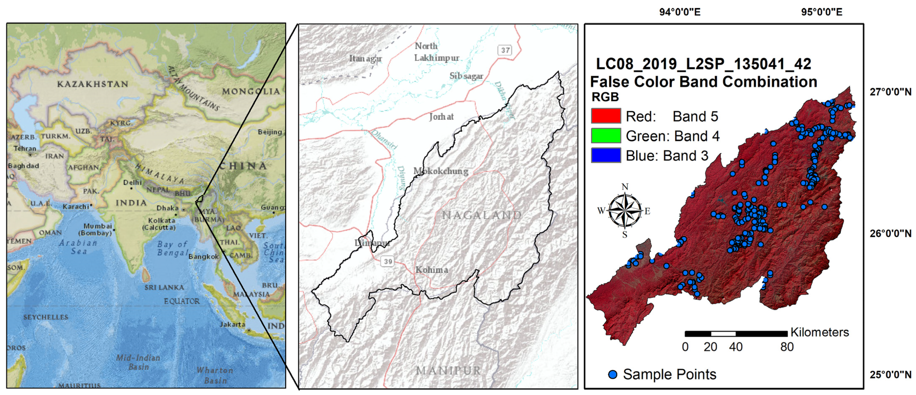
2.1. Study Area and Soil Data

The study was conducted in the state of Nagaland, located in the extreme eastern part of the Himalayan region of India (Figure 1). Nagaland is bounded by Myanmar to the east, Assam to the west and north, Arunachal Pradesh to the north, and Manipur to the south [31]. The study area (Figure 1) is approximately 17,000 km² and is located between 25°10′ N and 27°4′ N Latitude and 93°15′ E and 95°20′ E Longitude. The altitudinal range in Nagaland varies from 100 m to 3826 m a.s.l. [32]. The climate type of the region is mainly Cwa (monsoon-influenced humid subtropical climate) according to the Köppen–Geiger climate classification system [33]. Nagaland is primarily a hilly state, stretching in a narrow strip from northeast to southwest, and located in the northern extension of the Arakan Yoma Mountain ranges of Myanmar. The forest cover of Nagaland encompasses approximately 12,000 km², representing 73.91% of its total area [34]. ‘Shifting cultivation’, locally known as ‘jhum’, is the second major land use in the state, following forest cover [35]. The primary crop grown in the state is upland rice (Oryza sativa) using conventional practices, which serve as a staple food. Other significant crops include maize, cowpea, pulses, and vegetables [36]. The majority of soils in the region can be classified as Inceptisols according to the USDA Soil Taxonomy [37], with Ultisols being the second most common soil order.

From 2013 to 2017, soil surveys were conducted in various districts of Nagaland to gather soil samples from a depth of 0–30 cm. A total of 305 sites were randomly selected under different land uses, and the GPS was used to record the sampling positions of all the sites (Figure 1). At each site, a quadrat of 10 m × 10 m was laid, and five samples (four at the corners and one at the center) were collected to make a composite sample. The collected soil samples were air-dried at room temperature (22 °C), grinded, and passed through a 2-mm sieve to exclude litter, roots, and coarse particles. CEC was measured by 1 N ammonium acetate (pH 7.0) method [38].

2.2. Digital Covariates

This study utilized DEM-based terrain attributes, satellite image-based indexes, and climate data to represent environmental conditions and their influence on the distribution of soil CEC.

The System for Automated Geoscientific Analysis (SAGA) GIS [39] was employed to calculate the topographic digital covariates from the digital elevation model (DEM) [40], In addition, remote sensing-based indices were derived from Landsat 8 OLI surface reflectance (SR) [41] data by applying band operations [42]. Climate variables were obtained from the “WorldClim 2” dataset [43].

Table 1. Digital covariates used for estimating soil cation exchange capacity.

Covariate Name	Definition		Refs.
Elevation	Elevation, measured as height above sea level		[40]
Slope	Slope measures the elevation change and steepness of a line		[39]
Pl-cur	Rate of change of aspect along a contour		[39]
Pr-cur	Rate of change of slope down a slope line		[39]
Con-Ind	Calculated using flow direction and neighboring cell aspects		[39]
Flow-acc	Calculated accumulated flow		[39]
Val-depth	The vertical height below the summit accumulation		[39]
Flow-dir	Height differences between cells determine the flow direction.		[39]
MRVBF	The measure of flatness and lowness depicting depositional areas		[44]
MRRTF	The measure of flatness and upness depicting stable upland areas		[44]
TWI	The measure of the propensity of an area to accumulate water		[39,45]
TPI	Difference between a cell elevation value and the average elevation of the neighborhood around that cell		[39]
TRI	Degree of roughness or irregularity of the landscape		[39]
NDVI Stdv, Median, Mean	$\left(NIR Band-Red Band\right)/\left(NIR Band+Red Band\right)$	(1)	[46]
	Measures the amount and health of vegetation in a given area
RONR Stdv, Median, Mean	$\left(SWIR Band-Green Band\right)/\left(SWIR Band+Green Band\right)$	(2)
Landsat 8 OLI ProductIDs	LC08_L2SP_135041_20170204_20200905_02_T1, LC08_L2SP_135042_20170204_20200905_02_T1		[41]
	LC08_L2SP_135041_20190125_20200829_02_T1, LC08_L2SP_135042_20190125_20200830_02_T1
BIO-1	The annual mean temperature in degrees Celsius.		[43]
BIO-12	Annual precipitation in millimeters.
TSR	Thirty-year mean solar radiation in 12 months in kJ m−2 year−1

Note: NDVI: Normalized Difference Vegetation Index, RONR: Rock Outcrop Normalized Ratio, BIO-1: Mean Annual Temperature (MAT), BIO-12: Annual Precipitation, TSR: Total Solar Radiation, Pl-cur: Planform Curvature, Pr-Cur: Profile Curvature, Con-Ind: Convergence Index, Flow-acc: Flow Accumulation, Val-depth: Valley Depth, Flow-dir: Flow Direction, MRVBF: Multi-resolution valley bottom flatness index, MRRTF: Multi-resolution of ridge top flatness index, TWI: Topographic wetness index, TPI: Topographic position index, TRI: Topographic roughness index.

contains information on the digital covariates used in the study.

All the digital covariates were standardized through a disaggregation approach (based on the nearest neighbors’ technique) to the same pixel resolution of 30 m and the same extent and were reprojected onto the epsg:32646 projection system [42].

2.3. Modelling Cation Exchange Capacity

This study followed the DSM framework and was conducted in several steps (Figure 2): (1) Soil data enabling and data curation process, (2) acquisition of digital covariates from open-sources, (3) extraction of georeferenced sample points from the digital covariates data and preparation of geodatabases, (4) selection of the digital covariates using the “caretFuncs” functions for each algorithm, (5) iteratively employing ML models, and (6) producing predictive mean and standard deviation maps. Figure 2 shows the flowchart of the present study.

To reduce the redundancy among digital covariates and to produce a model with a parsimony approach [47], the recursive feature elimination (rfe) process in accordance with root mean square error (RMSE) minimization (Figure A1) was employed while taking into account the available digital covariates (Table 1). The digital covariates selection process was carried out for each machine learning algorithm using the “caretFuncs” [48] function.

Five ML models (Table 2) were systematically compared to identify the relationships between soil CEC and digital covariates for the study area. K Nearest neighbors (KNN) [49], gradient boosting machine (GBM) [50,51], Lasso regression (LR) [52], random forest (RF) [53,54], and support vector regression (SVR) [55,56] were executed. These ML algorithms were chosen because the mathematical differences on which they are based can be easily compared using the scientific literature [22,25], whether they are linear or not.

The K-nearest neighbor (KNN) algorithm is a supervised ML algorithm useful for solving regression problems [49]. As in this study, if the values of the target function are “continuous”, the process proceeds by calculating the mean. For solving a regression problem, Nearest-neighbor methods utilize the observations in the calibration set that is closest in input space to $x$ to form $Y$;

$$Y \left(x\right)=\frac{1}{k} {{\displaystyle \sum }}_{x_{i }\in N_k\left(x\right)}yi,$$

(3)

where $N_k\left(x\right)$ represents the neighborhood of $x$, defined as the k closest points $x_{i }$ in the training sample. The notion of closeness is based on a metric, which in this case is assumed to be the Euclidean distance. Thus, we find the k observations closest to $x$ in input space and take the average of their responses. The optimization of the model’s performance in the study involved the tuning parameter closest instances (k).

The random forest (RF) algorithm is an ensemble learning method for regression problems [54]. Introduced by Breiman [54], it is an improvement over the bootstrap aggregating (bagging) algorithm. The idea behind RF is to build multiple decision trees and use them to make predictions. The final prediction is made by aggregating the predictions of all the trees, and the average in a regression model. For a more detailed understanding of the RF method, see Biau and Scornet [57]. Out of Bag (OOB) errors were computed using 36.8% of the training dataset to evaluate variable importance. Mean square error (MSE) was employed as the prediction error in the OOB analysis for regression models, with the software generating two critical measures: %IncMSE and IncNodePurity. %IncMSE was computed for each tree with and without relevant predictors, and the mean differences were normalized to their standard deviation. IncNodePurity represents the average total reduction in node impurity from splitting among predictors in the tree-building process across all trees, with node impurity measured using residual sum of squares [58]. The optimization of the model’s performance in the study involved the tuning parameter of the number of possible directions for splitting at each node of each tree “mtry”.

Gradient Boosting Machine (GBM) is an ensemble learning method that combines the predictions from multiple weak models to produce a stronger final prediction [50]. GBM uses an ensemble learning method but uses boosting rather than bagging. Instead of focusing on the complete training data, boosting algorithms select only a fraction of the training data to improve prediction accuracy gradually. The optimization of the model’s performance in the study involved the tuning of parameters, including terminal node size (n.minobsinnode), number of trees (n.trees), number of splits (interaction.depth), and learning rate (shrinkage).

Lasso regression (LR) is a type of regularized or penalized regression model that is particularly useful for dealing with multicollinearity in datasets where the number of variables is high [59]. This helps to prevent overfitting and improves the interpretability of the model. In mathematical terms, the LR can be expressed as an optimization problem where the objective function is the sum of the mean squared error and the Lasso penalty term. The Lasso penalty term is defined as the sum of the absolute values of the regression coefficients, multiplied by a tuning parameter that controls the strength of the regularization. The optimization problem is solved using numerical methods, such as coordinate descent, to find the values of the regression coefficients that minimize the objective function [60]. The optimization of the model’s performance in the study involved the tuning of the penalty parameter (Lambda).

Support vector regression (SVR) is a type of supervised learning algorithm that can be used for regression tasks. SVR works by mapping the input data to a high-dimensional feature space and then finding a hyperplane that best fits the data in that space [55]. SVR aims to find a hyperplane that fits the data while allowing for some errors. The optimization problem involves finding the hyperplane that maximizes the margin between the support vectors and the hyperplane while minimizing the prediction error. This is done by solving a set of Lagrange multipliers that are used to define the support vectors and the hyperplane. Once the optimization problem is solved, the support vectors define the boundary of the hyperplane, and the model can be used to make predictions on new data points. The optimization of the model’s performance in the study involved the tuning of parameters regularization constant (C) and kernel width parameter (sigma).

Hyperparameters of each ML algorithm were tuned using their respective packages (Table 2).

Using R Core Environment software (Version 4.2.1) [61] and RStudio IDE [62], the CEC of the surface soil in the study area was estimated using a laboratory soil analysis dataset and selected digital covariates in Table 2. Iterative models were created by the process of a 10-fold CV. The average outcomes of these models were used to create the final soil CEC map based on each ML algorithm.

Table 2. Parameters of the machine learning algorithms used and final digital covariates included to model CEC.

Algorithm	Digital Covariates	R Package	Tuning Hyperparameter
KNN	BIO-1, BIO-12, Elevation, TSR, TRI, NDVI-Mean, TPI, Slope, Pr-cur, Val-depth, Con-Ind	caret [63]	k: 9
LR	BIO-1, BIO-12, Elevation	glmnet [52,64]	Lambda: 0.56
RF	BIO-1, BIO-12, Elevation, TSR	randomForest [65]	mtry: 2
GBM	BIO-1, BIO-12, Elevation	gbm [51]	shrinkage: 0.32, interaction.depth: 9, n.minobsinnode: 8, n.trees: 272
SVR	BIO-1, BIO-12, Elevation, TSR	e1071 [66]	Sigma: 0.74, cost: 1

Note: LR: Lasso regression, GBM: Stochastic gradient boosting, SVR: Support vector regression, RF: Random forest, KNN: K-nearest neighbors.

Table 2. Parameters of the machine learning algorithms used and final digital covariates included to model CEC.

Algorithm	Digital Covariates	R Package	Tuning Hyperparameter
KNN	BIO-1, BIO-12, Elevation, TSR, TRI, NDVI-Mean, TPI, Slope, Pr-cur, Val-depth, Con-Ind	caret [63]	k: 9
LR	BIO-1, BIO-12, Elevation	glmnet [52,64]	Lambda: 0.56
RF	BIO-1, BIO-12, Elevation, TSR	randomForest [65]	mtry: 2
GBM	BIO-1, BIO-12, Elevation	gbm [51]	shrinkage: 0.32, interaction.depth: 9, n.minobsinnode: 8, n.trees: 272
SVR	BIO-1, BIO-12, Elevation, TSR	e1071 [66]	Sigma: 0.74, cost: 1

Note: LR: Lasso regression, GBM: Stochastic gradient boosting, SVR: Support vector regression, RF: Random forest, KNN: K-nearest neighbors.

2.4. Model Performance Evaluation and Uncertainty Analysis

Model output and observations were compared with statistics from cross-validation [67]. A 10-fold cross-validation with 5 repetitions was used [68]. The determination coefficient (R²) was used to evaluate the model validation, along with mean absolute error (MAE) and root mean square error (RMSE) [68]. The formulas for these parameters are as follows:

$$\mathrm{MAE}=\frac{{{\displaystyle \sum }}_{i=1}^n\left|\mathrm{O}i-\mathrm{P}i\right|}{n}$$

(4)

$$\mathrm{RMSE}=\sqrt{\frac{{{\displaystyle \sum }}_{i=1}^n{\left(\mathrm{O}i-\mathrm{P}i\right)}^2}{n}}$$

(5)

$${\mathrm{R}}^2={\left[\frac{{{\displaystyle \sum }}_{i=1}^n\left(\mathrm{O}i-\mathrm{O}ave\right)\left(\mathrm{P}i-\mathrm{P}ave\right)}{\sqrt{{{\displaystyle \sum }}_{i=1}^n{\left(\mathrm{O}i-\mathrm{O}ave\right)}^2{\left(\mathrm{P}i-\mathrm{P}ave\right)}^2}}\right]}^2$$

(6)

where O_i and P_i are, respectively, the observed and predicted values, with their average values represented by O_ave and P_ave, respectively, and n is the sample size in the dataset.

The accuracy of a digital soil map can be evaluated at locations where soil samples were collected and analyzed. On the other hand, the uncertainty associated with a soil map can be estimated for each raster cell or pixel in the map [68]. In the current study, uncertainty was estimated by calculating the standard deviation of predictions for each pixel across the 10 model runs. This represents the degree of variation in the predicted values within each pixel around the mean value [69,70].

3. Results

3.1. Soil CEC Data Summary Statistics

Figure 3 depicts the statistical distribution of CEC characteristics in the study area, including a histogram and Q-Q plot of the soil samples. Mean CEC was 12.11 cmol_c kg⁻¹, with an amplitude ranging from 1.79 to 30.23 cmol_c kg⁻¹, a standard deviation of 5.26 cmol_c kg⁻¹, and a median of 11.31 cmol_c kg⁻¹, as shown in Figure 3. The determined coefficient of variation of 43.46% is relatively high (Figure 3). The skewness and kurtosis values of the CEC were close to 0. Based on the results of the Grubbs’ Test [71] with a 5% level of significance, no outliers were present in the dataset (G value is 3.44; p value is 0.156).

3.2. Performance of Different Machine Learning Algorithms

Figure 4 and

Table 3. Evaluation criteria for the machine learning algorithms included root mean square error (RMSE), mean absolute error (MAE), and R-squared (R²) values.

Criteria	Model	Mean	Standard Deviation	Median
RMSE	RF	4.12	0.56	4.13
	SVR	4.27	0.51	4.13
	KNN	4.45	0.66	4.46
	LR	4.67	0.75	4.55
	GBM	5.07	0.55	5.11
R2	RF	0.41	0.13	0.40
	SVR	0.36	0.11	0.34
	KNN	0.30	0.12	0.31
	LR	0.25	0.16	0.26
	GBM	0.25	0.12	0.26
MAE	RF	3.12	0.42	3.21
	SVR	3.29	0.38	3.29
	KNN	3.44	0.49	3.38
	LR	3.56	0.55	3.44
	GBM	4.01	0.42	4.00

Note: LR: Lasso regression, GBM: Stochastic gradient boosting, SVR: Support vector regression, RF: Random forest, KNN: K-nearest neighbors.

show 10-fold statistics from cross-validation for the soil CEC predictions of the study at soil surface.

The mean RMSE values for CEC according to cross-validation statistics of the models ranged from 4.12 to 5.07, while R² values ranged from 0.25 to 0.41 and MAE values ranged from 3.12 to 4.01, as shown in Table 3. Figure 4 displays the variation in R², MAE, and RMSE values during cross-validation of the models. The RF model outperformed the other models, demonstrating lower RMSE and MAE values, and higher R² values compared to the other models as shown in Table 3 and Figure 4. The standard deviations of these performance criteria were highest with LR (0.75, 0.16, and 0.55 for RMSE, R², and MAE, respectively) (Table 3).

3.3. Predictive Maps of CEC and Quantified Uncertainties

We used five ML models to generate maps of the spatial distribution of soil CEC in the study area. The average CEC estimate produced by each algorithm and the spatial distribution of uncertainty (standard deviation) based on 10 times bootstrapping are presented in separate subsections. By zooming to the different physiography compared, the five algorithms were found to have robust effects on soil CEC mapping.

3.3.1. Mapping CEC Content and Its Uncertainty via RF

The soil CEC digital map created using the RF algorithm and four climate digital covariates (Table 2) showed that extreme CEC values could not be represented spatially (Figure 5b). The RF model estimated the CEC values in the range of 5–15 cmol_c kg⁻¹ in the younger and older alluvial plain areas but was not able to capture the high variability in these areas (Figure 5a). However, in the highly/moderately dissected hills and valley physiography (Figure 5c), the RF model could separate the sample points in the range of 5–15 cmol_c kg⁻¹ and 15–25 cmol_c kg⁻¹ relatively well. The uncertainty of the CEC values was lower in the central and northeastern regions, where more soil samples were collected, and higher in the southwest and southeast regions with fewer soil observations.

3.3.2. Mapping CEC Content and Its Uncertainty via SVR

The mean CEC predict map generated by the SVR algorithm using four climate digital covariates (Table 2) produced similar results to RF, with both algorithms unable to represent extreme CEC values spatially. In younger and older alluvial plain area, both models estimated CEC values in the range of 5–15 cmol_c kg⁻¹ and failed to capture high variability. The SVR model performed relatively well in separating sample points between 5–15 cmol_c kg⁻¹ and 15–25 cmol_c kg⁻¹ in high/medium dissected hills and valley physiography. The uncertainty of CEC values was higher in the southwest and southeast regions with fewer soil observations, resulting in higher standard deviation values than with RF (Figure 6e).

3.3.3. Mapping CEC Content and Its Uncertainty via LR

The LR algorithm, using two climate and one topography digital covariates (Table 2), generated a mean CEC estimation map (Figure 7b) that produced similar results to RF and SVR, but could not represent spatial extreme CEC values. The LR model estimated CEC values in the range of 5–15 cmol_c kg⁻¹ in the younger and older alluvial plain area and failed to capture high variability. In addition, the LR model performed relatively worse than RF and SVR in separating values between 5–15 cmol_c kg⁻¹ and 15–25 cmol_c kg⁻¹ in high/medium dissected hills and valleys physiography (Figure 7c).

3.3.4. Mapping CEC Content and Its Uncertainty via GBM

As in LR, the mean CEC estimation map was created by the GBM algorithm of two climates and one topography digital covariates (Table 2) that produced different results from LR, RF, and SVR throughout the study area and represented the extreme CEC values on more digital maps than the others provided. In a younger and older alluvial plain area, the GBM model, like the others, estimated CEC values in the range of 5–15 cmol_c kg⁻¹ and could not achieve high variability. The GBM model performed relatively better than LR in separating between 5–15 cmol_c kg⁻¹ kg and 15–25 cmol_c kg⁻¹ in high/medium dissected hills and valley physiography and provided the limits with more details (Figure 8c).

3.3.5. Mapping CEC Content and Its Uncertainty via KNN

The KNN model was used to estimate the CEC using three climatic, one vegetation, and seven topographic covariates, thus it produced the CEC map with the highest number of digital covariates (Table 2). The mean CEC prediction map created with the KNN model showed different distributions throughout the study area compared to other models but was similar to SVR. However, the KNN model was relatively unsuccessful in representing extreme CEC values except for GBM, (Figure 9a). The KNN model, like the other models, estimated CEC values in the range of 5–15 cmol_c kg⁻¹ in a younger and older alluvial plain area and did not provide high variability. In the high/medium dissection hills and valley physiography, the KNN model performed relatively better than LR in distinguishing between 5–15 cmol_c kg⁻¹ and 15–25 cmol_c kg⁻¹, providing more detailed limits (Figure 9c).

3.4. Importance of Digital Covariates in Modelling Process

The relative importance graphs of the digital covariates used in the RF model, which provides the most ideal results, and the LR model with the highest SD value, are given in Figure 10. The BIO-1 annual mean temperature covariate was found to be the most important feature in all the models, regardless of whether they were linear or non-linear. According to the feature importance rankings of the two ML models, the three most important variables in descending order were the BIO-1 annual mean temperature, elevation, and total solar radiation.

4. Discussion

4.1. Systematic Evaluation of the Five Machine-Learning Models

We compared our 10-fold–five-repetition model performance statistics, which were made with five different ML algorithms, with published studies conducted in similar regions [19] and at different scales [72]. In the current study, the tree-based machine learning model RF achieved better performance statistical values than KNN, SVR, LR, and GBM (Table 3). More recently, Reddy and Das [19], using similar digital covariates in their CEC estimation and mapping study across India, reported R² around 0.60 and RMSE around 9.00 cmol_c kg⁻¹. In Burkina Faso, Forkuor et al. [26] compared the efficacy of similar set of digital covariates and RF, SVR, GBM, and multiple linear regression (MLR) algorithms to predict CEC, and achieved the highest performance with RMSE values of 4.69 cmol_c kg⁻¹ and R² 0.38. Chagas et al. [73] achieved a R² value of 0.47 with the RF model and RMSE of 7.89 cmol_c kg⁻¹, while Dharumarajan et al. [72] obtained R² 0.52 and RMSE 13:07 cmol_c kg⁻¹ in topsoil (0–30 cm). Nascimento et al. [74] achieved R² 0.19 and RMSE 3.26 cmol_c kg⁻¹ in their study in which they included satellite data for many years as a variable for CEC estimation in the Sao Paulo region of Brazil. Khanal et al. [25] compared the efficacy of multi-band aerial photographs and high spatial resolution DEM derivatives and Linear regression, RF, Neural networks (NN), SVR, GBM, and Cubist models to predict CEC at the field scale. They reported that the algorithm obtained R² 0.67 and RMSE 2.35 cmol_c kg⁻¹ performance statistical values via NN algorithm. The RF-based digital soil CEC map produced in the present study used topographic derivatives, the mean values of plant and soil-based indices produced from time-series satellite images (Landsat 8 OLI), and open access climate data, and the effectiveness of our model procedure was confirmed by comparing the performances of the models in the existing literature. We can recommend a high resolution (30 m) CEC map for Nagaland state as an informative starting point to guide future new sampling, considering model performance statistics.

4.2. Physiography and Soil Cation Exchange Capacity

It is well known that topsoil CEC is highly influenced by topography, which tends to be higher overall in areas of sedimentation or deposition [20]. In addition, the geochemistry of the parent material also significantly influences CEC values [19]. Considering the spatial resolution of the digital covariates that were used in the study, and that we did not have a quantitative geology map, we could not add this variable as a predictive raster covariate [31]. Thus, we considered that the evaluation of the predictive maps in two different physiographic areas that dominate the study region can provide important insights. The presence of 1:1 kaolinite clay in gneiss formations may explain the low clay values in these soils. However, the presence of smectite (2:1 type clays) of different parent material origin in alluvial areas partially explains the presence of high CECs. In terms of the qualitative evaluation of the predictive map, no algorithm was successful from the soil scientist point of view to represent the CEC values in alluvial areas (Figure 5a, Figure 6a, Figure 7a, Figure 8a and Figure 9a). Natural disturbances such as flooding in alluvial areas are the ultimate cause of this disagreement, as this affects the distribution of soil particle fractions over very short distances, significantly affecting the distribution of clay, which is one of the most important factors on which CEC depends. The current study area has a highly variable topography and is characterized by dissected deep valleys and hills, which determine soil property and landscape variability. In particular, dissected hills and valleys may have different CEC values as a result of mass movement, periodic flooding, and accumulation of multiple material resources. The digital maps produced in the study area by five different algorithms show a significant difference especially in relation LR and GBM. Thus, while these two algorithms are involved in CEC mapping with the same digital covariates (Table 2), they produce very different CEC digital maps. This is proof that no single algorithm is “best” in the field DSM [29]. In particular, the current study makes significant contributions to the literature by producing CEC prediction and uncertainty [10,67,75] maps in surface soils and evaluating them in detail through the eyes of soil scientists.

4.3. Factors Affecting Soil Cation Exchange Capacity

The variable importance is significant for interpreting the models obtained from the soil scientist perspective and providing useful information for future modeling approaches [76]. In the modeling, ML models were run in line with the covariates selected with “rfe” due to the tight approach, and the importance graphs of the variables used in the model of RF, which produced the most successful model performance statistics, and LR, which produced the most unsuccessful maps, were analyzed (Figure 10). Interestingly, the most important variable in both algorithms was BIO-12, followed by elevation. Considering the nature of the study area, the variables valued by the linear or nonlinear algorithm were the same. The effectiveness of climate variables in CEC mapping in India is particularly compatible with the findings of Reddy and Das [19]. Similarly, Akpa et al. [22], working in similar geographies in Nigeria, identified precipitation, temperature, and elevation digital covariates as the most important in the CEC estimation. Shaded hillsides typically exhibit lower light intensity, evaporation rates, and air and soil temperatures, with less frequent soil freezing and thawing compared to sunny slopes. Consequently, soils on shaded hillsides demonstrate increased water penetration at greater depths relative to those on predominantly sunny hillsides. However, the intensity of weathering is reduced on colder, shaded hillsides. These justifications may explain the relationship of solar total radiation and annual mean temperature with soil physicochemical properties in the present study area. Similar outcomes have been reported in other studies [77]. The vegetation of our current study area covers the soil throughout the year [78] and the spatial resolution (30 m) of the satellite image used may have had difficulty reflecting the heterogeneity in the area. Failure to reflect the heterogeneity of data on vegetation or organisms remotely sensed by satellite can present difficulties in CEC prediction models over large areas [79]. In the study area, transport of clay during the monsoonal season into deeper layers and the process of clay pedogenesis significantly drives the spatial distribution of CEC in the surface soil.

4.4. Limitations and Perspectives

Although the evaluation of the performance statistics of the models confirms the relative usefulness of soil CEC estimates and maps, particularly through the RF algorithm, uncertainties and limitations remain associated with this study. Specifically, Gray et al. [27] recommend using a detailed geology map for DSM-based mapping of soil properties whenever available. Accordingly, incorporating a detailed geological map into the model can improve performance statistics of models and reduce map uncertainty at smaller scale studies within the Nagaland state. The selection of a soil sampling method can significantly impact the quality of characterizing spatial variability in soil properties [80]. Considering technical advancements in cost-effective smart sampling techniques for assessing soil sampling density in heterogeneous areas, careful consideration of appropriate sampling strategies is imperative prior to undertaking DSM [81]. The methodology can be advanced by checking the digital covariate values (for example, temperature, solar radiation, elevation, and NDVI) in the soil sampling points provided as training data with the covariate values throughout the study area, especially in large areas (such as our study area), with techniques such as Multivariate Environmental Similarity Surfaces (MESS) [82,83,84] before modeling. In future research, it is recommended to use multispectral remote sensing data with higher spatial resolution [23] as well as various ancillary data such as synthetic aperture radar (SAR), especially to represent vegetation. The collection and analysis of such data is critical for future research to accurately characterize the spatio-temporal dynamics of the soil CEC. Many machine learning algorithms that have parallel computing power, such as Extreme Gradient Boosting (XGBoost) [85], can be evaluated in terms of efficiency, such as shortening the modeling time [86] which can help in studies with large datasets in large areas.

5. Conclusions

To address the lack of knowledge about the spatial distributions of cation exchange capacity (CEC) in the highly mountainous and all year-round vegetation-dominated Nagaland state of India, five machine learning (ML) model predictions and spatial uncertainties were derived and systematically evaluated from a soil scientist perspective. The RF model exhibited superior performance relative to the other models, as evidenced by lower RMSE (4.12 cmol_c kg⁻¹) and MAE (3.12 cmol_c kg⁻¹) values and higher R² (0.41) values. The results required the careful use of models to spatially detect CEC value ranges in young and old alluvial deposits, which are one of the dominant physiography of the area. Due to the tropical environmental conditions of the region, climatic variables were determined as indispensable CEC estimators. As flexible and stable models, tree learners—such as random forest models—provided strong performance and outperformed others in model performance statistics. In addition, the results confirm that there is no single ML that can be used to map soil features, especially in areas of dissected hills and valleys. Future sampling efforts should focus on areas where high standard deviations were found, to minimize current uncertainty in surface CEC modeling. This study is the first of its kind in the state and is deemed much needed by soil scientists and land planners in Nagaland. While this work will provide a national CEC content base map for Nagaland, it can serve as a good reference work to develop CEC content mapping in similar physiographic settings.

References

1. Hou, D.; Bolan, N.S.; Tsang, D.C.W.; Kirkham, M.B.; O’Connor, D. Sustainable Soil Use and Management: An Interdisciplinary and Systematic Approach. Sci. Total Environ. 2020, 729, 138961. [Google Scholar] [CrossRef] [PubMed]
2. Hou, D. Sustainable Soil Management for Food Security. Soil Use Manag. 2023, 39, 1–7. [Google Scholar] [CrossRef]
3. Zhao, X.; Arshad, M.; Li, N.; Zare, E.; Triantafilis, J. Determination of the Optimal Mathematical Model, Sample Size, Digital Data and Transect Spacing to Map CEC (Cation Exchange Capacity) in a Sugarcane Field. Comput. Electron. Agric. 2020, 173, 105436. [Google Scholar] [CrossRef]
4. Mishra, G.; Sulieman, M.M.; Kaya, F.; Francaviglia, R.; Keshavarzi, A.; Bakhshandeh, E.; Loum, M.; Jangir, A.; Ahmed, I.; Elmobarak, A.; et al. Machine Learning for Cation Exchange Capacity Prediction in Different Land Uses. Catena 2022, 216, 106404. [Google Scholar] [CrossRef]
5. Moulatlet, G.M.; Zuquim, G.; Figueiredo, F.O.G.; Lehtonen, S.; Emilio, T.; Ruokolainen, K.; Tuomisto, H. Using Digital Soil Maps to Infer Edaphic Affinities of Plant Species in Amazonia: Problems and Prospects. Ecol. Evol. 2017, 7, 8463–8477. [Google Scholar] [CrossRef]
6. Levis, C.; Costa, F.R.C.; Bongers, F.; Peña-Claros, M.; Clement, C.R.; Junqueira, A.B.; Neves, E.G.; Tamanaha, E.K.; Figueiredo, F.O.G.; Salomão, R.P.; et al. Persistent Effects of pre-Columbian Plant Domestication on Amazonian Forest Composition. Science 2017, 355, 925–931. [Google Scholar] [CrossRef]
7. Cambule, A.H.; Rossiter, D.G.; Stoorvogel, J.J. A Methodology for Digital Soil Mapping in Poorly-Accessible Areas. Geoderma 2013, 192, 341–353. [Google Scholar] [CrossRef]
8. Heuvelink, G.B.M.; Webster, R. Modelling Soil Variation: Past, Present, and Future. Geoderma 2001, 100, 269–301. [Google Scholar] [CrossRef]
9. Iticha, B.; Takele, C. Soil–Landscape Variability: Mapping and Building Detail Information for Soil Management. Soil Use Manag. 2018, 34, 111–123. [Google Scholar] [CrossRef]
10. Rossiter, D.G. Soil Mapping Today: Computer-Generated Predictive Soil Maps-Their Role in Soil Survey and Land Evaluation. Agric. Dev. 2021, 44, 5. [Google Scholar]
11. Burke, M.; Lobell, D.B. Satellite-Based Assessment of Yield Variation and Its Determinants in Smallholder African Systems. Proc. Natl. Acad. Sci. USA 2017, 114, 2189–2194. [Google Scholar] [CrossRef] [Green Version]
12. Huggett, R. Soil as Part of the Earth System. Prog. Phys. Geogr. 2023. [Google Scholar] [CrossRef]
13. Huggett, R.J. Soil as a System. In Hydrogeology, Chemical Weathering, and Soil Formation; American Geophysical Union (AGU): Washington, DC, USA, 2021; pp. 1–20. ISBN 9781119563952. [Google Scholar]
14. Minasny, B.; McBratney, A.B. Digital Soil Mapping: A Brief History and Some Lessons. Geoderma 2016, 264, 301–311. [Google Scholar] [CrossRef]
15. Scull, P.; Franklin, J.; Chadwick, O.A.; McArthur, D. Predictive Soil Mapping: A Review. Prog. Phys. Geogr. Earth Environ. 2003, 27, 171–197. [Google Scholar] [CrossRef] [Green Version]
16. Brevik, E.C.; Calzolari, C.; Miller, B.A.; Pereira, P.; Kabala, C.; Baumgarten, A.; Jordán, A. Soil Mapping, Classification, and Pedologic Modeling: History and Future Directions. Geoderma 2016, 264, 256–274. [Google Scholar] [CrossRef]
17. Grunwald, S.; Böhner, J. Geographical Information Systems (GIS) and Soils. Ref. Modul. Earth Syst. Environ. Sci. 2022. [Google Scholar] [CrossRef]
18. Sorenson, P.T.; Kiss, J.; Bedard-Haughn, A.K.; Shirtliffe, S. Multi-Horizon Predictive Soil Mapping of Historical Soil Properties Using Remote Sensing Imagery. Remote Sens. 2022, 14, 5803. [Google Scholar] [CrossRef]
19. Reddy, N.N.; Das, B.S. Digital Soil Mapping of Key Secondary Soil Properties Using Pedotransfer Functions and Indian Legacy Soil Data. Geoderma 2023, 429, 116265. [Google Scholar] [CrossRef]
20. Ballabio, C.; Lugato, E.; Fernández-Ugalde, O.; Orgiazzi, A.; Jones, A.; Borrelli, P.; Montanarella, L.; Panagos, P. Mapping LUCAS Topsoil Chemical Properties at European Scale Using Gaussian Process Regression. Geoderma 2019, 355, 113912. [Google Scholar] [CrossRef]
21. Hengl, T.; Heuvelink, G.B.M.; Kempen, B.; Leenaars, J.G.B.; Walsh, M.G.; Shepherd, K.D.; Sila, A.; MacMillan, R.A.; de Jesus, J.M.; Tamene, L.; et al. Mapping Soil Properties of Africa at 250 m Resolution: Random Forests Significantly Improve Current Predictions. PLoS ONE 2015, 10, e0125814. [Google Scholar] [CrossRef]
22. Akpa, S.I.C.; Ugbaje, S.U.; Bishop, T.F.A.; Odeh, I.O.A. Enhancing Pedotransfer Functions with Environmental Data for Estimating Bulk Density and Effective Cation Exchange Capacity in a Data-Sparse Situation. Soil Use Manag. 2016, 32, 644–658. [Google Scholar] [CrossRef]
23. Liu, F.; Wu, H.; Zhao, Y.; Li, D.; Yang, J.L.; Song, X.; Shi, Z.; Zhu, A.X.; Zhang, G.L. Mapping High Resolution National Soil Information Grids of China. Sci. Bull. 2022, 67, 328–340. [Google Scholar] [CrossRef] [PubMed]
24. Saidi, S.; Ayoubi, S.; Shirvani, M.; Azizi, K.; Zeraatpisheh, M. Comparison of Different Machine Learning Methods for Predicting Cation Exchange Capacity Using Environmental and Remote Sensing Data. Sensors 2022, 22, 6890. [Google Scholar] [CrossRef] [PubMed]
25. Khanal, S.; Fulton, J.; Klopfenstein, A.; Douridas, N.; Shearer, S. Integration of High Resolution Remotely Sensed Data and Machine Learning Techniques for Spatial Prediction of Soil Properties and Corn Yield. Comput. Electron. Agric. 2018, 153, 213–225. [Google Scholar] [CrossRef]
26. Forkuor, G.; Hounkpatin, O.K.L.; Welp, G.; Thiel, M. High Resolution Mapping of Soil Properties Using Remote Sensing Variables in South-Western Burkina Faso: A Comparison of Machine Learning and Multiple Linear Regression Models. PLoS ONE 2017, 12, e0170478. [Google Scholar] [CrossRef] [Green Version]
27. Gray, J.M.; Bishop, T.F.A.; Wilford, J.R. Lithology and Soil Relationships for Soil Modelling and Mapping. Catena 2016, 147, 429–440. [Google Scholar] [CrossRef]
28. Sawicka, K.; Heuvelink, G.B.M.; Walvoort, D.J.J. Spatial Uncertainty Propagation Analysis with the Spup R Package. R J. 2018, 10, 180–199. [Google Scholar] [CrossRef] [Green Version]
29. Rossiter, D.G.; Poggio, L.; Beaudette, D.; Libohova, Z. How Well Does Digital Soil Mapping Represent Soil Geography? An Investigation from the USA. SOIL 2022, 8, 559–586. [Google Scholar] [CrossRef]
30. Miller, B. Referee Comment on “How Well Does Digital Soil Mapping Represent Soil Geography? An Investigation from the USA” by David G. Rossiter et al. SOIL 2022, 8, 559–586. [Google Scholar] [CrossRef]
31. GON Government of Nagaland. Available online: https://nagaland.gov.in/ (accessed on 4 August 2022).
32. Mishra, G.; Francaviglia, R. Land Uses, Altitude and Texture Effects on Soil Parameters. A Comparative Study in Two Districts of Nagaland, Northeast India. Agriculture 2021, 11, 171. [Google Scholar] [CrossRef]
33. Beck, H.E.; Zimmermann, N.E.; McVicar, T.R.; Vergopolan, N.; Berg, A.; Wood, E.F. Present and Future Köppen-Geiger Climate Classification Maps at 1-Km Resolution. Sci. Data 2018, 5, 180214. [Google Scholar] [CrossRef] [Green Version]
34. STATE OF FOREST REPORT 2021. Forest Survey of India (Ministry of Environment Forest and Climate Change): Dehradun, IN. 2021. Available online: https://fsi.nic.in/forest-report-2021-details (accessed on 15 January 2023).
35. Singh, A.K.; Bordoloi, L.J.; Kumar, M.; Hazarika, S.; Parmar, B. Land Use Impact on Soil Quality in Eastern Himalayan Region of India. Environ. Monit. Assess. 2014, 186, 2013–2024. [Google Scholar] [CrossRef]
36. Mishra, G.; Das, J.; Sulieman, M. Modelling Soil Cation Exchange Capacity in Different Land-Use Systems Using Artificial Neural Networks and Multiple Regression Analysis. Curr. Sci. 2019, 116, 2020–2027. [Google Scholar] [CrossRef]
37. Soil Survey Staff. Keys to Soil Taxonomy, 12th ed.; USDA-Natural Resources Conservation Service: Washington, DC, USA, 2014. [Google Scholar]
38. Sumner, M.E.; Miller, W.P. Cation Exchange Capacity and Exchange Coefficients. In Methods of Soil Analysis, Part 3: Chemical Methods; Soil Science Society of America, Inc. and American Society of Agronomy, Inc.: Madison, WI, USA, 1996; pp. 1201–1229. ISBN 9780891188667. [Google Scholar]
39. Conrad, O.; Bechtel, B.; Bock, M.; Dietrich, H.; Fischer, E.; Gerlitz, L.; Wehberg, J.; Wichmann, V.; Böhner, J. System for Automated Geoscientific Analyses (SAGA) v. 2.1.4. Geosci. Model Dev. 2015, 8, 1991–2007. [Google Scholar] [CrossRef] [Green Version]
40. NASA Shuttle Radar Topography Mission (SRTM) Shuttle Radar Topography Mission (SRTM) Global. Distributed by OpenTopography; OpenTopography: La Jolla, CA, USA, 2013. [CrossRef]
41. Sayler, K.; Glynn, T. Landsat 8 Collection 2 (C2) Level 2 Science Product (L2SP) Guide LSDS-1619 Version 2.0; EROS Sioux Falls: South Dakota, SD, USA, 2021. [Google Scholar]
42. ESRI. ArcGIS User’s Guide. 2023. Available online: http://www.esri.com (accessed on 15 January 2023).
43. Fick, S.E.; Hijmans, R.J. WorldClim 2: New 1-Km Spatial Resolution Climate Surfaces for Global Land Areas. Int. J. Climatol. 2017, 37, 4302–4315. [Google Scholar] [CrossRef]
44. Gallant, J.C.; Dowling, T.I. A Multiresolution Index of Valley Bottom Flatness for Mapping Depositional Areas. Water Resour. Res. 2003, 39, 1347. [Google Scholar] [CrossRef]
45. Moore, I.D.; Gessler, P.E.; Nielsen, G.A.; Peterson, G.A. Soil Attribute Prediction Using Terrain Analysis. Soil Sci. Soc. Am. J. 1993, 57, 443–452. [Google Scholar] [CrossRef]
46. Brown, K.S.; Libohova, Z.; Boettinger, J. Digital Soil Mapping. In Soil Survey Manual; Ditzler, C., Scheffe, K., Monger, H.C., Eds.; USDA Handbook 18; Government Printing Office: Washington, DC, USA, 2017. [Google Scholar]
47. Poggio, L.; de Sousa, L.M.; Batjes, N.H.; Heuvelink, G.B.M.; Kempen, B.; Ribeiro, E.; Rossiter, D. SoilGrids 2.0: Producing Soil Information for the Globe with Quantified Spatial Uncertainty. SOIL 2021, 7, 217–240. [Google Scholar] [CrossRef]
48. Kuhn, M. caretFuncs: Backwards Feature Selection Helper Functions. In caret R Package Version 6.0-86. 2020. Available online: https://CRAN.R-project.org/package=caret (accessed on 15 January 2023).
49. Hastie, T.; Tibshirani, R.; Friedman, J. Overview of Supervised Learning. In The Elements of Statistical Learning: Data Mining, Inference, and Prediction; Springer: New York, NY, USA, 2009; pp. 9–41. [Google Scholar] [CrossRef]
50. Friedman, J.H. Stochastic Gradient Boosting. Comput. Stat. Data Anal. 2002, 38, 367–378. [Google Scholar] [CrossRef]
51. Greenwell, B.; Boehmke, B.; Cunningham, J. gbm: Generalized Boosted Regression Models. 2020. Available online: https://cran.r-project.org/web/packages/gbm/gbm.pdf (accessed on 15 January 2023).
52. Friedman, J.; Hastie, T.; Tibshirani, R. Regularization Paths for Generalized Linear Models via Coordinate Descent. J. Stat. Softw. 2010, 33, 1. [Google Scholar] [CrossRef] [Green Version]
53. Breiman, L. Statistical Modeling: The Two Cultures. Stat. Sci. 2001, 16, 199–321. [Google Scholar] [CrossRef]
54. Breiman, L. Random Forests. Mach. Learn. 2001, 45, 5–32. [Google Scholar] [CrossRef] [Green Version]
55. Drucker, H.; Burges, C.J.; Kaufman, L.; Smola, A.; Vapnik, V. Support Vector Regression Machines. Adv. Neural Inf. Process. Syst. 1996, 9, 155–161. [Google Scholar]
56. Chang, C.C.; Lin, C.J. LIBSVM: A library for support vector machines. ACM Trans. Intell. Syst. Technol. 2011, 2, 1–27. [Google Scholar] [CrossRef]
57. Biau, G.; Scornet, E. A Random Forest Guided Tour. Test 2016, 25, 197–227. [Google Scholar] [CrossRef] [Green Version]
58. Keshavarzi, A.; del Árbol, M.Á.S.; Kaya, F.; Gyasi-Agyei, Y.; Rodrigo-Comino, J. Digital Mapping of Soil Texture Classes for Efficient Land Management in the Piedmont Plain of Iran. Soil Use Manag. 2022, 38, 1705–1735. [Google Scholar] [CrossRef]
59. Ferhatoglu, C.; Miller, B.A. Choosing Feature Selection Methods for Spatial Modeling of Soil Fertility Properties at the Field Scale. Agronomy 2022, 12, 1786. [Google Scholar] [CrossRef]
60. Murphy, K.P. Sparse Linear Models. In Machine Learning: A Probabilistic Perspective; The MIT Press: London, UK, 2012; pp. 421–479. [Google Scholar]
61. R Core Team. R: A Language and Environment for Statistical Computing. R Foundation for Statistical Computing. Available online: https://www.r-project.org/ (accessed on 15 January 2023).
62. RStudio Team. RStudio: Integrated Development for R. RStudio, PBC, Boston, MA. Available online: http://www.rstudio.com/ (accessed on 15 January 2023).
63. Kuhn, M. Caret: Classification and Regression Training. R Package Version 6.0-86. 2020. Available online: https://CRAN.R-project.org/package=caret (accessed on 15 January 2023).
64. Simon, N.; Friedman, J.; Hastie, T.; Tibshirani, R. Regularization Paths for Cox’s Proportional Hazards Model via Coordinate Descent. J. Stat. Softw. 2011, 39, 1. [Google Scholar] [CrossRef]
65. Liaw, A.; Wiener, M. Classification and Regression by RandomForest. R News 2002, 2, 18–22. [Google Scholar]
66. Meyer, D.; Dimitriadou, E.; Hornik, K.; Weingessel, A.; Leisch, F. E1071: Misc Functions of the Department of Statistics, Probability Group (Formerly: E1071); TU Wien: Vienna, Austria, 2022. [Google Scholar]
67. Rossiter, D.G. Maps and Models Are Never Valid, but They Can Be Evaluated. Pedometron 2017, 41, 19–21. [Google Scholar]
68. Piikki, K.; Wetterlind, J.; Söderström, M.; Stenberg, B. Perspectives on Validation in Digital Soil Mapping of Continuous Attributes—A Review. Soil Use Manag. 2021, 37, 7–21. [Google Scholar] [CrossRef]
69. Bian, Z.; Guo, X.; Wang, S.; Zhuang, Q.; Jin, X.; Wang, Q.; Jia, S. Applying statistical methods to map soil organic carbon of agricultural lands in northeastern coastal areas of China. Arch. Agron. Soil Sci. 2020, 66, 532–544. [Google Scholar] [CrossRef]
70. Nalin, R.S.; Dalmolin, R.S.D.; de Araújo Pedron, F.; Moura-Bueno, J.M.; Horst, T.Z.; Schenato, R.B.; Soligo, M.F. Accounting for the Spatial Variation of Phosphorus Available Explained by Environmental Covariates. Geoderma Reg. 2023, 32, e00594. [Google Scholar] [CrossRef]
71. Komsta, L. Outliers: Tests for Outliers, Version 0.15. Available online: https://cran.r-project.org/web/packages/outliers/outliers.pdf (accessed on 5 January 2023).
72. Dharumarajan, S.; Kalaiselvi, B.; Suputhra, A.; Lalitha, M.; Hegde, R.; Singh, S.K.; Lagacherie, P. Digital Soil Mapping of Key GlobalSoilMap Properties in Northern Karnataka Plateau. Geoderma Reg. 2020, 20, e00250. [Google Scholar] [CrossRef]
73. Chagas, C.D.S.; de Carvalho Júnior, W.; Pinheiro, H.S.K.; Xavier, P.A.M.; Bhering, S.B.; Pereira, N.R.; Filho, B.C. Mapping Soil Cation Exchange Capacity in a Semiarid Region through Predictive Models and Covariates from Remote Sensing Data. Rev. Bras. Ciênc. Solo 2018, 42, 170183. [Google Scholar] [CrossRef]
74. Nascimento, C.M.; Demattê, J.A.M.; Mello, F.A.O.; Rosas, J.T.F.; Tayebi, M.; Bellinaso, H.; Greschuk, L.T.; Albarracín, H.S.R.; Ostovari, Y. Soil Degradation Detected by Temporal Satellite Image in São Paulo State, Brazil. J. S. Am. Earth Sci. 2022, 120, 104036. [Google Scholar] [CrossRef]
75. Liu, Y.; Heuvelink, G.B.M.; Bai, Z.; He, P. Uncertainty quantification of nitrogen use efficiency prediction in China using Monte Carlo simulation and quantile regression forests. Comput. Electron. Agric. 2023, 204, 107533. [Google Scholar] [CrossRef]
76. Fiorentini, M.; Schillaci, C.; Denora, M.; Zenobi, S.; Deligios, P.; Orsini, R.; Santilocchi, R.; Perniola, M.; Montanarella, L.; Ledda, L. A Machine Learning Modelling Framework for Triticum Turgidum Subsp. Durum Desf Yield Forecasting in Italy. Agron. J. 2022. [Google Scholar] [CrossRef]
77. Blume, H.-P.; Brümmer, G.W.; Fleige, H.; Horn, R.; Kandeler, E.; Kögel-Knabner, I.; Kretzschmar, R.; Stahr, K.; Wilke, B.-M. (Eds.) Soil Development and Soil Classification. In Scheffer/Schachtschabel Soil Science; Springer: Berlin/Heidelberg, Germany, 2016; pp. 285–389. [Google Scholar]
78. Mishra, G.; Marzaioli, R.; Giri, K.; Borah, R.; Dutta, A.; Jayaraj, R.S.C. Soil Quality Assessment under Shifting Cultivation and Forests in Northeastern Himalaya of India. Arch. Agron. Soil Sci. 2017, 63, 1355–1368. [Google Scholar] [CrossRef]
79. Zarnetske, P.L.; Read, Q.D.; Record, S.; Gaddis, K.D.; Pau, S.; Hobi, M.L.; Malone, S.L.; Costanza, J.; Dahlin, K.M.; Latimer, A.M.; et al. Towards Connecting Biodiversity and Geodiversity across Scales with Satellite Remote Sensing. Glob. Ecol. Biogeogr. 2019, 28, 548–556. [Google Scholar] [CrossRef] [Green Version]
80. Malone, B.; Arrouays, D.; Poggio, L.; Minasny, B.; McBratney, A. Digital Soil Mapping: Evolution, Current State and Future Directions of the Science. Ref. Modul. Earth Syst. Environ. Sci. 2022. [Google Scholar] [CrossRef]
81. Brus, D.J. Spatial Sampling with R; Chapman and Hall/CRC: Boca Raton, FL, USA, 2022; ISBN 9781003258940. [Google Scholar]
82. Broeg, T.; Blaschek, M.; Seitz, S.; Taghizadeh-Mehrjardi, R.; Zepp, S.; Scholten, T. Transferability of Covariates to Predict Soil Organic Carbon in Cropland Soils. Remote Sens. 2023, 15, 876. [Google Scholar] [CrossRef]
83. Silva, B.P.C.; Silva, M.L.N.; Avalos, F.A.P.; de Menezes, M.D.; Curi, N. Digital Soil Mapping Including Additional Point Sampling in Posses Ecosystem Services Pilot Watershed, Southeastern Brazil. Sci. Rep. 2019, 9, 13763. [Google Scholar] [CrossRef] [PubMed] [Green Version]
84. Camera, C.; Zomeni, Z.; Noller, J.S.; Zissimos, A.M.; Christoforou, I.C.; Bruggeman, A. A High Resolution Map of Soil Types and Physical Properties for Cyprus: A Digital Soil Mapping Optimization. Geoderma 2017, 285, 35–49. [Google Scholar] [CrossRef]
85. Zhang, M.; Shi, W.; Xu, Z. Systematic Comparison of Five Machine-Learning Models in Classification and Interpolation of Soil Particle Size Fractions Using Different Transformed Data. Hydrol. Earth Syst. Sci. 2020, 24, 2505–2526. [Google Scholar] [CrossRef]
86. Radočaj, D.; Jurišić, M.; Antonić, O.; Šiljeg, A.; Cukrov, N.; Rapčan, I.; Plaščak, I.; Gašparović, M. A Multiscale Cost-Benefit Analysis of Digital Soil Mapping Methods for Sustainable Land Management. Sustainability 2022, 14, 12170. [Google Scholar] [CrossRef]
Figure 1. The study site location and sampling points shown on a Landsat 8 OLI satellite image.
Land 12 00819 g001
Figure 2. A simplified flowchart outlining the research conducted in this study.
Land 12 00819 g002
Figure 3. Histogram and Q-Q plot of measured CEC in the dataset.
Land 12 00819 g003
Figure 4. Comparison of model evaluation parameters: (a) root mean square error (RMSE), (b) coefficient of determination (R2), (c) mean absolute error (MAE). Calculations were performed over 10 iterations.
Land 12 00819 g004
Figure 5. Digital maps of CEC (0–30 cm) were generated by applying a random forest (RF) model: Zoomed to a young and older alluvial plain area as mean CEC map (a) and as uncertainty CEC map (d); mean CEC map over Nagaland (b) resulting from the prediction among 10 iterations; zoomed to a highly/moderately dissected hills and valleys as mean CEC map (c) and as uncertainty CEC map (f); uncertainty CEC map over Nagaland (e) resulting from the standard deviation of 10 iterations.
Land 12 00819 g005
Figure 6. Digital maps of CEC (0–30 cm) were generated by applying a Support Vector Regression (SVR) model: Zoomed to a young and older alluvial plain area as mean CEC map (a) and as uncertainty CEC map (d); mean CEC map over Nagaland (b) resulting from the prediction among 10 iterations; zoomed to a highly/moderately dissected hills and valleys as mean CEC map (c) and as uncertainty CEC map (f); uncertainty CEC map over Nagaland (e) resulting from the standard deviation of 10 iterations.
Land 12 00819 g006
Figure 7. Digital maps of CEC (0–30 cm) were generated by applying a Lasso Regression (LR) model: Zoomed to a young and older alluvial plain area as mean CEC map (a) and as uncertainty CEC map (d); mean CEC map over Nagaland (b) resulting from the prediction among 10 iterations; zoomed to a highly/moderately dissected hills and valleys as mean CEC map (c) and as uncertainty CEC map (f); uncertainty CEC map over Nagaland (e) resulting from the standard deviation of 10 iterations.
Land 12 00819 g007
Figure 8. Digital maps of CEC (0–30 cm) were generated by applying a Stochastic Gradient Boosting (GBM) model: Zoomed to a young and older alluvial plain area as mean CEC map (a) and as uncertainty CEC map (d); mean CEC map over Nagaland (b) resulting from the prediction among 10 iterations; zoomed to a highly/moderately dissected hills and valleys as mean CEC map (c) and as uncertainty CEC map (f); uncertainty CEC map over Nagaland (e) resulting from the standard deviation of 10 iterations.
Land 12 00819 g008
Figure 9. Digital maps of CEC (0–30 cm) were generated by applying a K-nearest neighbors (KNN) model: Zoomed to a young and older alluvial plain area as mean CEC map (a) and as uncertainty CEC map (d); mean CEC map over Nagaland (b) resulting from the prediction among 10 iterations; zoomed to a highly/moderately dissected hills and valleys as mean CEC map (c) and as uncertainty CEC map (f); uncertainty CEC map over Nagaland (e) resulting from the standard deviation of 10 iterations.
Land 12 00819 g009
Figure 10. Variable importance for RF (a,b) and LR (c).
Land 12 00819 g010