Abstract
Food is increasingly seen as a vehicle to address complex sustainability challenges, where the quantitative driving role in balancing the complex urban system of socio-economy and environment is still a gap. To fill this gap, taking Shanghai city as an example, this paper utilizes system dynamics to innovatively set three policy scenarios that aim at adjusting food security and cultivated land resources. The results confirm their positive role in socioeconomic and environmental improvement and coordinated development. In the high-rate grain yield growth scenario, the labor force ratio of the primary industry increases back to the size of 2012 (4.1%), the proportion of the primary industrial investment grows at twice the rate of the current trend, the grain yield per unit area increases back to the capacity of 1997 (798.154 t/km2), and simultaneously, the occupation of cultivated land resources by the secondary industry and the negative impact of environmental pollution on productivity are mitigated. In that case, the coordination level between the socio-economy and the environment can keep increasing. The results indicate that future urban planning should increase the input of labor force and assets in the primary industry, improve food productivity per unit area through technical means or person training, alleviate the occupation of cultivated land resources by the secondary industry, and mitigate the negative impact of environmental pollution on cultivated land productivity.
1. Introduction
Humans have entered the urban century [1]. The scale of the urban population worldwide reached 4.22 billion in 2018 and will keep growing to 6.68 billion in 2050 [2]. Urban development simultaneously creates more than 75% of the global GDP and contributes to 75% of energy-based carbon emissions [3]. Therefore, the urban population is the protagonist in the challenge for achieving sustainable development, as it carries most human activities connected with environmental crises and resource depletion. The New Urban Agenda at the Habitat III conference emphasized the role of cities as engines for sustainable development [4]. The knowledge about a sustainable future from an urban perspective should be central, and building a global urban science is essential [5]. Therefore, research on urban-scale development is of great significance for sustainable goals and science.
Further, realizing sustainable goals is not only the independent progress of each goal but, more importantly, to combat undesirable interactions, conflicts, and impacts, which can exactly be reflected in system analysis [6]. The urban system is a complex system and seeks systematic thinking [7]. System approaches can reduce negative surprises and promote integrated planning, management, and governance [8]. Therefore, it has been a research priority for some scholars to fully connect the urban socioeconomic and environmental systems and understand their dynamic interplay and feedback [9].
Among elements in different subsystems of complex urban system models, the resource mainly covers water resources [10,11], energy resources [12], nonrenewable and renewable resources [13], land use [14,15], and land development [16]. However, rapid urban development and sprawl are also threatening agricultural sustainability [17]. Although making cities sustainable is a global determination, little attention has been paid by the government to agriculture due to the belief that the highest benefit use of land is not on agriculture; this may result from a lack of the literature on the precise role of urban agriculture in building sustainable cities [18]. Therefore, considering the cultivated land elements in the complex urban system is of great theoretical significance.
A few studies on urban development take cultivated land resources and grain output into account [19]. Tapia et al. evaluated urban sustainability in Arhus based on an indicator framework that includes urban agriculture and food security [20]. Nigussie et al. analyzed the capacity and suitability of urban farmland in Ethiopia to contribute to sustainable development [21]. Tong et al. explored the manner to optimize urban food production in Tucson, a semi-arid region [22]. Xia et al. quantified the dynamics of green infrastructure in agriculture in Zhengzhou from the perspective of ecological security and food security [23]. Clerino et al. examined the practices for the sustainability assessment of professional urban agriculture [24]. Gozdziewicz-Biechonska et al. analyzed theoretical frameworks and practices for protecting agricultural land use [25]. These studies consider the element role of cultivated land and grain in sustainability. However, there is still a gap in their driving role in the coordinated development of complex urban systems.
Indeed, food is increasingly being regarded as a vehicle to simultaneously address economic, social, and environmental dilemmas [26]. Urban agriculture is recognized as a potential contributor to more sustainable development at the city level as it promotes food security and food sovereignty [27]. It is also lauded for its potential positive impacts on all three pillars of sustainability [18]. However, the effect of agriculture on the urban scale can be conflicting as good or bad [28]. The positive impacts include enhancing dietary diversity and improving ecosystem services and social quality [18,29,30], while the negative impacts are also stressed by some critics [27,31]. These arguments make it urgent to identify the role of food and cultivated land resources in the coordinated development of complex urban systems. In addition, although food resources for a metropolis can basically be supplied through trade with neighboring regions, the risk of public health events and natural disasters should be considered, and urban farming should be emphasized to increase food safety [32].
To sum up, this paper aims to fill the gap of the quantitative driving role of food and cultivated land resource in balancing the complex urban system of the socio-economy and the environment. Taking Shanghai city as an example, the system dynamics model is applied to simulate complex urban system development. Different scenarios are set to adjust the conditions of food and cultivated land resource and forecast the coordination level. According to the simulation results, suggestions for more sustainable and coordinated development are proposed from the perspectives of food security and cultivated land protection.
2. Methods and Study Area
2.1. System Dynamics Model
This paper applies system dynamics, which is an effective method for developing an understanding of complex systems [33]. This method can incorporate various elements of different subsystems in an integrated model, and the feedback loop can quickly seize the complex interactions [13]. In addition, scenario simulation is a good tool for policy or scheme analysis [10,34]. Due to these advantages, system dynamics has been applied in broad fields, including the urban system analysis, such as urban water–energy–food system [32], urban economy–resource–environment system [19], green urban system [35], urban social economy–water environment system [11], urban economy–society–resource–environment system [36], etc. Accordingly, this paper takes advantage of system dynamics to analyze the food role of urban agriculture in the urban system for coordination development between the socio-economy and the environment.
2.1.1. Model Conceptualization
This paper establishes an urban system, as shown in Figure 1. Firstly, this paper focuses on the food role in the coordination development of the urban system, reflected in 77 loops. For example:
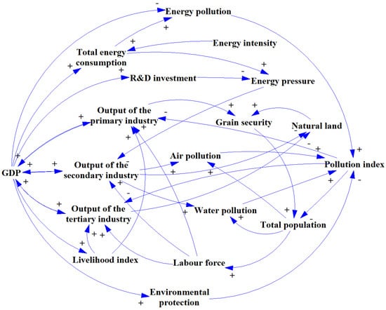
Figure 1.
Causal loop diagram of the urban system.
- Grain security→Total population→Labor force→Output of the primary industry→Grain security (a positive loop);
- Grain security→Total population→Labor force→Output of tertiary/secondary industry→natural land→Grain security (a negative loop);
- Grain security→Total population→Air/Water pollution→Pollution index→Output of the primary industry→Grain security (a negative loop);
- Grain security→Total population→Labor force→Output of the tertiary/secondary industry→GDP→Output of the primary industry (a positive loop);
- Grain security→Total population→Air/Water pollution→Pollution index→Output of the tertiary/secondary industry→GDP→Output of the primary industry (a negative loop).
Secondly, this paper hopes to provide a reference for promoting coordination development, considering the subsystems of the socio-economy and the environment. The socio-economy mainly covers the population, livelihood, three industries, and technology investment. The environmental subsystem investigates air and water pollution, energy consumption, and investment in protection.
2.1.2. Model Formulation
Based on the causal loop diagram, this paper further defines the urban system with various elements and interacting formulations (Appendix A). Then, the stock and flow chart of the system model is formulated, as shown in Figure 2. The model builds an urban system and aims to examine how the evolution of grain security (grain yield per capita) will influence the system coordination level. The determination methods of parameters in the interactions are shown in Appendix B.
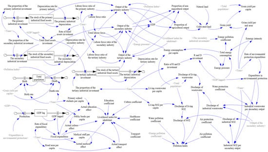
Figure 2.
Stock and flow chart of the urban system.
To confirm the model’s accuracy, this paper compares the simulated results with the actual data through the following formulas [19].
MARE represents Mean Absolute Relative Error, and a smaller value inflects a higher matching degree and a better simulation validation. is the actual value of indicator at time t, and is the simulated one.
2.1.3. Scenario Settings
After establishing the urban system, the food role of urban agriculture is examined. To this end, three scenarios have been designed, as shown in Table 1. The first is the current scenario, with all variables evolving as the current trend. The second is the scenario of high protection in urban agriculture, with related parameters being adjusted to promote the growth of grain yield at a higher rate than the current value. The third scenario is low protection in urban agriculture, where the grain yield grows at a lower rate or decreases.

Table 1.
Parameter setting of three scenarios to examine food role.
2.2. Coupling Coordination Degree Model
To evaluate the coordination level between the urban socio-economy and the environment, this paper applies the coupling coordination degree model, a widely use method for complex systems with various interactions [37,38,39].
2.2.1. Indicator System and Data Source
Firstly, the indicator system of the urban system is established in consideration of data accessibility and previous studies [35,36,40,41], as shown in Table 2. This paper mainly collects data from Shanghai Statistical Yearbooks, and the simulation span is 1995–2030. To ensure the results are reasonable, this paper applies indicators of per capita value and converts the ones related to currency into values with 2000 as the base year.
Table 2.
Indicator system of the urban system.
2.2.2. Performance Evaluation of Subsystems
Then, the performance of the socio-economy and environment is evaluated in the following three steps.
Step 1: The indicator values are standardized with the two formulas to eliminate the possible impacts of dimensions.
where and represent data before and after standardization, and and represent the maximum and minimum data of indicator .
Step 2: The weights of indicators are obtained with the entropy method.
Step 3: The performance levels are obtained.
2.2.3. Coordination Evaluation of the Urban System
Finally, the coordination level of the urban system is evaluated with the coupling coordination model.
where and are the performance level of the socio-economy and the environment, and and represent their contributions, respectively. The values of and are both 0.5 [37].
Based on previous studies [19,37], the coordination degree can be divided into five levels, i.e., seriously unbalanced (0 ≤ D < 0.25), slightly unbalanced (0.25 ≤ D < 0.5), barely balanced (0.5 ≤ D < 0.75), and superior balanced (0.75 ≤ D ≤ 1).
2.3. Study Area
Shanghai, a cosmopolitan megacity, is located at 120°52′~122°12′ E and 30°40′~31°53′ N. It has absorbed about 25 million people with a total area of 6340.5 km2. It plays a central role in multi-aspects of national development, such as the economy, technology, finance, etc. Therefore, it is significant for China and the world to study sustainable and coordinated development in Shanghai city. Since 2010, the Shanghai Municipal Government has made many efforts in farmland supplement and reclamation of inefficient construction land. However, there are still problems, such as insufficient reserve resources of agricultural land and contradiction of land use. Thus, agricultural land protection and food security are still severe.
3. Results
3.1. Model Accuracy
This paper compares the simulated results with the actual data to confirm the model’s accuracy. The average relative errors of these representative indicators are all within 5%, as shown in Figure 3; these results mean that the simulation values have good agreement with the actual values [34]. Therefore, the model’s behavior is reliable for simulating the development of Shanghai.
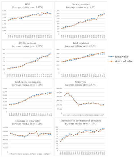
Figure 3.
Average relative error of some key indicators in the model.
3.2. Model Results of Three Scenarios
3.2.1. Development of Food in Urban Agriculture
Under different scenarios, cultivated land will perform differently, as shown in Figure 4. If Shanghai follows the current development trend, agricultural land resources will be increasingly severe, and the lower-rate grain yield growth scenario will see a more serious situation. In contrast, the higher-rate grain yield growth scenario can somewhat protect cultivated land and promote resource increase at a gentle rate.
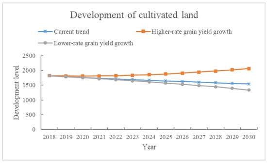
Figure 4.
Development of cultivated land under three scenarios.
Similarly, the development of grain yield per capita sees the same development trends, as shown in Figure 5. Therefore, the higher-rate grain yield growth scenario that is set by this paper can protect cultivated land resources and ensure food security.
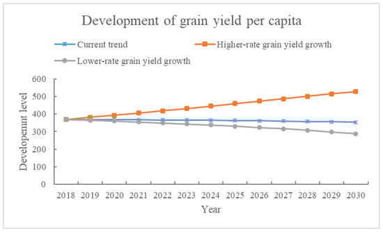
Figure 5.
Development of grain yield per capita under three scenarios.
3.2.2. Socioeconomic and Environmental Performance
Under different scenarios, the performance of the socio-economy and the environment in Shanghai differs. As shown in Figure 6, the socio-economy shows an upward trend under all three scenarios during 2018–2030. The lower-rate grain yield growth scenario shows a minimum rise from 0.32 to 0.55. In contrast, the performance under higher-rate grain yield increases significantly from 0.32 to 0.67. The results imply that ensuring food security benefits socioeconomic development, which can be explained through the indicators’ weights, as shown in Table 2. The top three important indicators are birth (32.47%), R & D expenditure per capita (23.55%), and the proportion of agriculture in GDP (15.93%), contributing to over 70% of the socioeconomic growth in total. High grain yield brings high growth in agriculture and promotes population growth, resulting in a high socio-economy. Therefore, the socioeconomic performances ranks are shown below: scenario under higher-rate grain yield growth > current scenario > scenario under lower-rate grain yield growth.
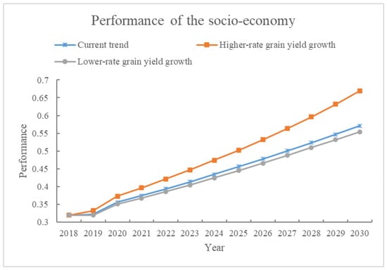
Figure 6.
Performance of the socio-economy under three scenarios.
For the environment, the performance shows an opposite trend during 2018–2030, as shown in Figure 7. It will decrease sharply from 0.66 to 0.32 on the current development trend, and the situation under lower-rate grain yield growth will be even more serious. By comparison, the environmental performance can almost maintain the present level under higher-rate grain yield growth. The results imply that ensuring food security can also benefit environmental development, which can be explained through the indicators’ weights in Table 2. Grain yield per capita and cultivated land per capita contribute to 23.32% and 11.95% of environmental performance, respectively; this is one-third in total. Therefore, the environmental performance ranks are shown below: scenario under higher-rate grain yield growth > current scenario > scenario under lower-rate grain yield growth.
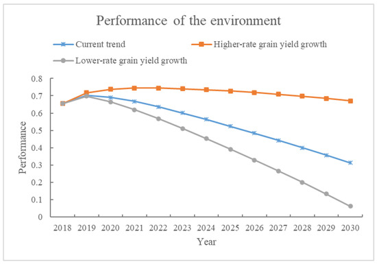
Figure 7.
Performance of the environment under three scenarios.
3.2.3. Coupling Coordination Level
The coupling degrees under three scenarios are shown in Figure 8, reflecting the interacting intensity between the socio-economy and the environment. The trends under the current and higher-rate yield growth scenarios are similar, increasing from 0.2 to almost 1. In contrast, the coupling degree under lower-rate grain yield scenario growth sharply declines after 2027 to the original level.
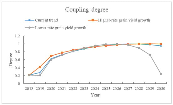
Figure 8.
Coupling degree under three scenarios.
The coordination degrees under three scenarios are shown in Figure 9. In general, the coordination levels under current and higher-rate grain yield growth scenarios show an upward trend, while that of the under lower-rate grain yield growth scenario begins to decrease after 2025. Specifically, the coordination level of the current scenario increases gently from 0.3 (slightly unbalanced) to 0.7 (barely balanced). Coordination of higher-rate grain yield growth scenario is the highest and increases significantly to 0.967 (superior balanced). In contrast, that of the lower-rate grain yield growth is the lowest and first increases slowly to slightly unbalanced by 2025, and then, falls back to slightly unbalanced by 2030. These results indicate that neglecting the food role of urban agriculture will lead to uncoordinated development.
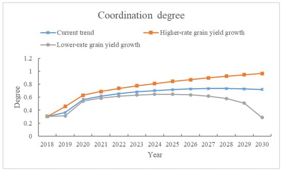
Figure 9.
Coordination degree under three scenarios.
4. Discussion
Firstly, we can confirm the food role of urban agriculture in promoting the socio-economy by comparing the prediction results of different scenarios (Figure 6). The high-rate grain yield growth scenario promotes investment in the labor force and assets of the primary industry as well as improves the efficiency of food production. In addition, it alleviates the secondary industry’s occupation of cultivated land resources and the negative impact of environmental damage on cultivated productivity. All these adjustments can promote the proportion of agriculture in GDP and have a positive effect on population development, which are essential aspects of the socioeconomic subsystem. These discoveries are in line with previous studies. Strengthening the development of food resources has been proven to be an optimized scenario to improve food security and GDP per capita [34]. Urban agriculture significantly benefits economic stability and physical health [42].
Secondly, we can also confirm the food role of urban agriculture in promoting the environment by comparing the prediction results of different scenarios (Figure 7). The high-rate grain yield growth scenario reduces the investment in the labor force and assets of the secondary industry as well as improves environmental protection, which can reduce pollution emissions and energy consumption. In addition, it protects the cultivated land resources and enhances food security, which has already been recognized as feasible in rich regions [27]. All these adjustments can promote the environmental subsystem. These findings align with other studies that show that more sustainable urban food systems allow energy conservation and emission reduction [42]. The results also provide quantitative evidence for previous views that urban agriculture is essential to deal with environmental deterioration [43]. Agriculture presents the potential for meeting sustainable goals in reducing adverse environmental impacts [44].
Finally, the food role of urban agriculture in promoting coordinated development is confirmed by comparing the prediction results of different scenarios (Figure 8 and Figure 9). The high-rate grain yield growth scenario improves the performance of the socioeconomic subsystem, mitigates the decline in environmental performance, and ensures a high coupling degree, which promotes coordinated development. These discoveries further expand the previous research results, further identifying that improving food security can benefit the development of the socioeconomic and the environmental subsystems and their coordination level.
5. Policy Implications
Based on the simulation results, this paper attaches importance to agriculture and proposes the following suggestions for Shanghai city and other metropolises worldwide with tense cultivated land resources and food security capacity to improve sustainability. Food-focused urban planning has already been recommended in some countries [45].
Firstly, increase the input of the labor force and assets in the primary industry to promote its development and improve food security. In the high-rate grain yield growth scenario, the labor force ratio of the primary industry is set to increase back to the size of 2012, rather than fall to less than half of the current level; and the proportion of the primary industrial investment will grow at twice the rate of the current growth trend. Comprehensive means, including these measures, can significantly improve the performance of socioeconomic and environmental subsystems and promote their coordinated development.
Secondly, improve food production efficiency through technical means or manual training to promote the development of the primary industry and improve food security. In the high-rate grain yield growth scenario, the grain yield per unit area is set to increase back to the capacity of 1997, much faster than the current trend, which has been proven by simulation as an effective way to improve food security.
Thirdly, mitigate the occupation of cultivated land resources by the secondary industry. In the high-rate grain yield growth scenario, the labor force ratio of the secondary industry is set to decrease at a faster rate than the actual trend; the same is true for the proportion of the secondary industrial investment. Comprehensive means, including these measures, can also significantly improve the performance of socioeconomic and environmental subsystems and promote their coordinated development.
Last but not least, strengthen environmental protection and mitigate the negative impact of environmental damage on cultivated land production. In the high-rate grain yield growth scenario, the rate of environmental protection expenditure is set to increase faster than the current trend, which has been proven by simulation as an effective way to improve food security.
6. Conclusions
This paper applies system dynamics to innovatively analyze the quantitative role of food and cultivated land resources in complex urban systems of the socio-economy and the environment. Three scenarios, the current trend scenario, low-rate grain yield growth scenario, and high-rate grain yield growth scenario, are set to adjust food and cultivated land resources to analyze their roles. The coupling coordinated degree model is applied to evaluate the coordination level.
The results confirm the positive role of food and cultivated land resources in promoting the performance of socioeconomic and environmental subsystems in Shanghai city and coordinated development. The results indicate that future urban planning should increase the input of labor force and assets in the primary industry, improve food productivity per unit area through technical means or person training, alleviate the occupation of cultivated land resources by the secondary industry, and mitigate the negative impact of environmental pollution on cultivated land productivity.
It must be admitted that this study also has some limitations. The first limitation comes from data availability. For example, urban agriculture can also produce water pollution and play a role in promoting metabolism. However, due to the unavailability of data, these factors are not considered in the urban system. In addition to improving data quality, future research can continuously improve the representativeness of complex urban systems, such as incorporating the interactions between other elements as well as between different cities into the comprehensive system, making it more reflective of the actual development pattern.
Funding
This research was funded by the Fundamental Research Funds for the Central Universities (XJ2022003001).
Data Availability Statement
Not applicable.
Conflicts of Interest
The authors declare no conflict of interest.
Appendix A. Model Formulations
- [1]
- Air pollution coefficient = 0.81
- [2]
- Air protection coefficient = 0.2553
- [3]
- Birth = Birth rate × Total population × Grain yield per capita^0.3384
- [4]
- Birth rate ([(1995, 0)–(2030, 0.01)], (1995, 0.0055), (1996, 0.0056), (1997, 0.0055), (1998, 0.0052), (1999, 0.0054), (2000, 0.0053), (2001, 0.0043), (2002, 0.0047), (2003, 0.0043), (2004, 0.006), (2005, 0.0061), (2006, 0.006), (2007, 0.0073), (2008, 0.007), (2009, 0.0066), (2010, 0.0071), (2011, 0.0072), (2012, 0.0096), (2013, 0.0076), (2014, 0.0086), (2015, 0.0074), (2016, 0.009), (2017, 0.0081), (2018, 0.0067), (2030, 0.0085))
- [5]
- Cultivated land = Natural land × Proportion of agricultural output^0.2342/Proportion of nonagricultural outputt^8.975
- [6]
- Culture coefficient = 0.3105
- [7]
- Death = Death rate × Total population × (1 + Pollution index × 6.3084)/Grain yield per capita^0.3384
- [8]
- Death rate ([(1995, 0)–(2030, 0.01)], (1995, 0.0075), (1996, 0.007), (1997, 0.0068), (1998, 0.007), (1999, 0.0065), (2000, 0.0072), (2001, 0.0071), (2002, 0.0073), (2003, 0.0075), (2004, 0.0072), (2005, 0.0075), (2006, 0.0072), (2007, 0.0074), (2008, 0.0077), (2009, 0.0076), (2010, 0.0077), (2011, 0.0079), (2012, 0.0054), (2013, 0.0082), (2014, 0.0083), (2015, 0.0086), (2016, 0.0085), (2017, 0.0087), (2018, 0.0086), (2030, 0.0095))
- [9]
- Depreciation rate for primary industry = 0.045
- [10]
- Depreciation rate for secondary industry = 0.0698
- [11]
- Depreciation rate for tertiary industry = 0.045
- [12]
- Discharge of industrial SO2 = Output of the secondary industry × Industrial SO2 per secondary output/1000
- [13]
- Discharge of industrial wastewater = Output of the secondary industry × Industrial wastewater per secondary output
- [14]
- Discharge of living SO2 = Total population × Living SO2 per capita/1000
- [15]
- Discharge of living wastewater = Total population × Living wastewater per capita
- [16]
- Discharge OF SO2 = Discharge of industrial SO2 + Discharge of living SO2
- [17]
- Discharge of wastewater = Discharge of industrial wastewater + Discharge of living wastewater
- [18]
- Education coefficient = 0.1915
- [19]
- Energy intensity ([(1995, 0.8)–(2030, 2.2)], (1995, 1.0581), (1996, 1.0172), (1997, 0.9991), (1998, 1.0156), (1999, 1.0713), (2000, 1.125), (2001, 1.2388), (2002, 1.3188), (2003, 1.359), (2004, 1.3919), (2005, 1.4852), (2006, 1.5712), (2007, 1.6117), (2008, 1.6427), (2009, 1.6948), (2010, 1.7256), (2011, 1.7102), (2012, 1.8409), (2013, 1.9079), (2014, 1.7114), (2015, 1.7664), (2016, 1.7471), (2017, 1.8431), (2018, 1.855), (2019, 1.7215), (2030, 2.1033))
- [20]
- Energy pollution coefficient = Total energy consumption × 0.63/LN (The secondary industrial investment)
- [21]
- Energy consumption per capita = Total energy consumption/Total population
- [22]
- Energy pressure = Total energy consumption × 0.01/LN (R and D investment)
- [23]
- Expenditure in environmental protection = GDP lagged × Rate of environmental protection expenditure
- [24]
- FINAL TIME = 2030
- [25]
- Fiscal expenditure = GDP lagged × Rate of fiscal expenditure
- [26]
- GDP = Output of the primary industry + Output of the secondary industry + Output of the tertiary industry
- [27]
- GDP lag = INTEG (Production-GDP lagged,4151.4)
- [28]
- GDP lagged = GDP lag
- [29]
- Grain yield = Cultivated land × Grain yield per unit area
- [30]
- Grain yield per capita = Grain yield/Total population
- [31]
- Grain yield per unit area ([(1995, 370)–(2030, 800)], (1995, 725.517), (1996, 781.171), (1997, 798.154), (1998, 723.485), (1999, 715.366), (2000, 608.604), (2001, 539.629), (2002, 482.47), (2003, 383.793), (2004, 432.641), (2005, 443.995), (2006, 535.096), (2007, 530.097), (2008, 564.244), (2009, 601.483), (2010, 589.055), (2011, 610.972), (2012, 615.025), (2013, 607.181), (2014, 597.981), (2015, 590.516), (2016, 519.979), (2017, 520.772), (2018, 539.329), (2030, 762.012))
- [32]
- Healthcare coefficient = 0.129
- [33]
- Industrial SO2 per secondary output = 53.29 × EXP (−((Time − 1995)/19.46)^5)/(Expenditure in environmental protection^Air protection coefficient)
- [34]
- Industrial wastewater per secondary output = 1411 × EXP(−0.02637 × (Time − 1995))/(Expenditure in environmental protection^Water protection coefficient)
- [35]
- INITIAL TIME = 1995
- [36]
- Labor force ratio([(1995, 0.45)–(2030, 0.6)], (1995, 0.5617), (1996, 0.5838), (1997, 0.5639), (1998, 0.5416), (1999, 0.5113), (2000, 0.5082), (2001, 0.4763), (2002, 0.4886), (2003, 0.4946), (2004, 0.5521), (2005, 0.5333), (2006, 0.5396), (2007, 0.5334), (2008, 0.5328), (2009, 0.5239), (2010, 0.5213), (2011, 0.5126), (2012, 0.4976), (2013, 0.5923), (2014, 0.5709), (2015, 0.5527), (2016, 0.5353), (2017, 0.5217), (2018, 0.5095), (2030, 0.5316))
- [37]
- Labor force ratio of the primary industry ([(1995, 0.01)–(2030, 0.14)], (1995, 0.0985), (1996, 0.1204), (1997, 0.1271), (1998, 0.1244), (1999, 0.1141), (2000, 0.1077), (2001, 0.11), (2002, 0.1015), (2003, 0.0863), (2004, 0.0688), (2005, 0.063), (2006, 0.055), (2007, 0.0524), (2008, 0.0469), (2009, 0.0456), (2010, 0.034), (2011, 0.0338), (2012, 0.041), (2013, 0.037), (2014, 0.0328), (2015, 0.0338), (2016, 0.0333), (2017, 0.0309), (2018, 0.0297), (2030, 0.012))
- [38]
- Labor force ratio of the secondary industry ([(1995, 0.25)–(2030, 0.56)], (1995, 0.5447), (1996, 0.5226), (1997, 0.491), (1998, 0.4603), (1999, 0.4646), (2000, 0.4431), (2001, 0.3987), (2002, 0.3967), (2003, 0.4076), (2004, 0.4535), (2005, 0.4243), (2006, 0.4168), (2007, 0.4125), (2008, 0.4027), (2009, 0.3974), (2010, 0.4068), (2011, 0.403), (2012, 0.3944), (2013, 0.3501), (2014, 0.3492), (2015, 0.3377), (2016, 0.3285), (2017, 0.3136), (2018, 0.3074), (2030, 0.2782))
- [39]
- Labor force ratio of the tertiary industry ([(1995, 0.35)–(2030, 0.75)], (1995, 0.3568), (1996, 0.357), (1997, 0.3819), (1998, 0.4153), (1999, 0.4213), (2000, 0.4492), (2001, 0.4912), (2002, 0.5017), (2003, 0.5061), (2004, 0.4777), (2005, 0.5128), (2006, 0.5282), (2007, 0.5351), (2008, 0.5504), (2009, 0.557), (2010, 0.5592), (2011, 0.5632), (2012, 0.5646), (2013, 0.6129), (2014, 0.618), (2015, 0.6285), (2016, 0.6382), (2017, 0.6554), (2018, 0.663), (2030, 0.7098))
- [40]
- Livelihood index for inhabitant = LN (Fiscal expenditure × (Culture coefficient × Public books per capita + Education coefficient*Primary school students per capita + Healthcare coefficient × Medical staff per capita + Transport coefficient × Road area per capita))
- [41]
- Living SO2 per capita ([(1994, 0)–(2030, 12)], (1994, 6.402), (1995, 10.792), (1996, 5.307), (1997, 4.856), (1998, 6.417), (1999, 5.888), (2000, 8.585), (2001, 10.348), (2002, 7.105), (2003, 7.627), (2004, 6.736), (2005, 7.28), (2006, 6.808), (2007, 6.463), (2008, 6.917), (2009, 6.317), (2010, 4.121), (2011, 1.272), (2012, 1.46), (2013, 1.778), (2014, 1.351), (2015, 2.733), (2016, 0.283), (2017, 0.241), (2018, 0.033), (2019, 0.041), (2030, 0.131))
- [42]
- Living wastewater per capita ([(1994, 60)–(2030, 95)], (1994, 61.2117), (1995, 76.662), (1996, 78.8422), (1997, 74.6138), (1998, 77.3412), (1999, 75.0479), (2000, 75.345), (2001, 76.124), (2002, 74.257), (2003, 68.5793), (2004, 74.66), (2005, 78.6243), (2006, 89.3075), (2007, 86.7248), (2008, 84.9603), (2009, 85.6561), (2010, 91.8367), (2011, 65.6157), (2012, 72.0773), (2013, 73.5404), (2014, 73.0833), (2015, 73.3747), (2016, 76.1157), (2017, 74.6071), (2018, 74.5462), (2019, 74.1606), (2030, 77.1461))
- [43]
- Medical staff per capita([(1995, 0.005)–(2030, 0.011)], (1995, 0.0078), (1996, 0.0075), (1997, 0.0073), (1998, 0.0071), (1999, 0.0069), (2000, 0.0067), (2001, 0.0063), (2002, 0.0059), (2003, 0.0058), (2004, 0.0055), (2005, 0.0055), (2006, 0.0056), (2007, 0.0059), (2008, 0.006), (2009, 0.0059), (2010, 0.0059), (2011, 0.0059), (2012, 0.0062), (2013, 0.0065), (2014, 0.0068), (2015, 0.007), (2016, 0.0074), (2017, 0.0078), (2018, 0.0085), (2019, 0.0084), (2030, 0.0107))
- [44]
- Natural land = 6341
- [45]
- Output of the primary industry = 0.086/Pollution index^0.8284 × Livelihood index for inhabitant^0.1163 × The stock of the primary industrial fixed assets^0.91 × (Labor force ratio of the primary industry × Total labor force)^0.5272
- [46]
- Output of the secondary industry = 0.3843/Energy pressure^0.4549 × Energy consumption per capita^0.6016 × The stock of the secondary industrial fixed assets^0.8047 × (Total labor force*Labor force ratio of the secondary industry) ^0.3084
- [47]
- Output of the tertiary industry = 23.0808/Pollution index^0.8284 × Livelihood index for inhabitant^0.1163 × The stock of the tertiary industrial fixed assets^0.162 × (Total labor force × Labor force ratio of the tertiary industry) ^0.7136
- [48]
- Pollution index = LN (Energy pollution coefficient × (Air pollution coefficient × Discharge of SO2+Water pollution coefficient × Discharge of wastewater)/(Discharge of SO2+Discharge of wastewater))
- [49]
- Primary school students per capita([(1995, 0.02)–(2030, 0.08)], (1995, 0.0776), (1996, 0.0734), (1997, 0.0688), (1998, 0.063), (1999, 0.0556), (2000, 0.049), (2001, 0.0433), (2002, 0.0393), (2003, 0.0367), (2004, 0.0293), (2005, 0.0283), (2006, 0.0272), (2007, 0.0258), (2008, 0.0276), (2009, 0.0304), (2010, 0.0305), (2011, 0.0312), (2012, 0.032), (2013, 0.0328), (2014, 0.0331), (2015, 0.0331), (2016, 0.0326), (2017, 0.0325), (2018, 0.0342), (2019, 0.034), (2030, 0.0415))
- [50]
- Production = GDP-Expenditure in environmental protection
- [51]
- Proportion of agricultural output = Output of the primary industry/GDP
- [52]
- Proportion of nonagricultural output = (Output of the secondary industry + Output of the tertiary industry)/GDP
- [53]
- Public books per capita([(1995, 1)–(2030, 4)], (1995, 1.1216), (1996, 1.1392), (1997, 3.2102), (1998, 3.1493), (1999, 3.0989), (2000, 3.4191), (2001, 3.3974), (2002, 3.3959), (2003, 3.3378), (2004, 3.1891), (2005, 3.2005), (2006, 3.0866), (2007, 3.03), (2008, 2.9865), (2009, 2.9833), (2010, 2.9566), (2011, 2.9369), (2012, 3.0261), (2013, 2.9975), (2014, 3.035), (2015, 3.1337), (2016, 3.1719), (2017, 3.2146), (2018, 3.2567), (2019, 3.3208), (2030, 3.8485))
- [54]
- R and D investment = GDP lagged × Ratio of R and D investment
- [55]
- Rate of environmental protection expenditure ([(1995, 0)–(2030, 0.1)], (1995, 0.01846), (1996, 0.02309), (1997, 0.02376), (1998, 0.02666), (1999, 0.02642), (2000, 0.02949), (2001, 0.02909), (2002, 0.02802), (2003, 0.02815), (2004, 0.02782), (2005, 0.03057), (2006, 0.02933), (2007, 0.02843), (2008, 0.02906), (2009, 0.02925), (2010, 0.02833), (2011, 0.02788), (2012, 0.02827), (2013, 0.02814), (2014, 0.0277), (2015, 0.02636), (2016, 0.02756), (2017, 0.03015), (2018, 0.03027), (2019, 0.02829), (2030, 0.035))
- [56]
- Rate of fiscal expenditure ([(1995, 0.1)–(2030, 0.35)], (1995, 0.1064), (1996, 0.115), (1997, 0.1238), (1998, 0.1255), (1999, 0.1294), (2000, 0.1294), (2001, 0.1382), (2002, 0.1515), (2003, 0.1621), (2004, 0.1723), (2005, 0.1805), (2006, 0.1711), (2007, 0.1709), (2008, 0.1801), (2009, 0.1899), (2010, 0.1844), (2011, 0.1956), (2012, 0.2073), (2013, 0.2096), (2014, 0.1815), (2015, 0.2303), (2016, 0.2315), (2017, 0.2464), (2018, 0.2556), (2030, 0.3096))
- [57]
- Rate of fixed assets investment ([(1995, 0.1)–(2030, 0.7)], (1995, 0.6361), (1996, 0.6549), (1997, 0.5707), (1998, 0.5129), (1999, 0.4397), (2000, 0.3885), (2001, 0.3794), (2002, 0.3774), (2003, 0.3604), (2004, 0.3807), (2005, 0.3852), (2006, 0.3703), (2007, 0.3462), (2008, 0.3322), (2009, 0.335), (2010, 0.2968), (2011, 0.2532), (2012, 0.2604), (2013, 0.2614), (2014, 0.2381), (2015, 0.2363), (2016, 0.226), (2017, 0.2366), (2018, 0.2334), (2030, 0.1108))
- [58]
- Ratio of R and D investment ([(1995, 0.01)–(2030, 0.06)], (1995, 0.0129), (1996, 0.0137), (1997, 0.0144), (1998, 0.0145), (1999, 0.0151), (2000, 0.0159), (2001, 0.0168), (2002, 0.0177), (2003, 0.0189), (2004, 0.021), (2005, 0.0232), (2006, 0.0244), (2007, 0.0239), (2008, 0.0249), (2009, 0.0269), (2010, 0.0269), (2011, 0.0299), (2012, 0.0337), (2013, 0.036), (2014, 0.0341), (2015, 0.0348), (2016, 0.0351), (2017, 0.0393), (2018, 0.0416), (2030, 0.054))
- [59]
- Road area per capita ([(1995, 4)–(2030, 18)], (1995, 4.01), (1996, 4.46), (1997, 4.91), (1998, 6.04), (1999, 8.52), (2000, 8.68), (2001, 13.6), (2002, 11.6), (2003, 12.46), (2004, 15.36), (2005, 11.78), (2006, 11.84), (2007, 15.4), (2008, 15.7), (2009, 17.54), (2010, 11.12), (2011, 11.18), (2012, 11.24), (2013, 11.3), (2014, 11.51), (2015, 11.83), (2016, 12.09), (2017, 12.34), (2018, 12.49), (2019, 12.7), (2030, 14.63))
- [60]
- SAVEPER = TIME STEP
- [61]
- The primary industrial depreciation = The stock of the primary industrial fixed assets × Depreciation rate for primary industry
- [62]
- The primary industrial investment = Total fixed assets investment × The proportion of the primary industrial investment
- [63]
- The proportion of the primary industrial investment ([(1995, 0)–(2030, 0.012)], (1995, 0.0061), (1996, 0.0107), (1997, 0.004), (1998, 0.0033), (1999, 0.0044), (2000, 0.0044), (2001, 0.0035), (2002, 0.0025), (2003, 0.0018), (2004, 0.0018), (2005, 0.0017), (2006, 0.0037), (2007, 0.002), (2008, 0.0018), (2009, 0.0022), (2010, 0.0032), (2011, 0.0038), (2012, 0.0023), (2013, 0.0034), (2014, 0.0021), (2015, 0.0007), (2016, 0.0006), (2017, 0.0003), (2018, 0.0007), (2030, 0.0003))
- [64]
- The proportion of the secondary industrial investment ([(1995, 0)–(2030, 0.4)], (1995, 0.3226), (1996, 0.3314), (1997, 0.3354), (1998, 0.3333), (1999, 0.3323), (2000, 0.3294), (2001, 0.3427), (2002, 0.332), (2003, 0.3291), (2004, 0.3275), (2005, 0.3055), (2006, 0.309), (2007, 0.3135), (2008, 0.2942), (2009, 0.2707), (2010, 0.2699), (2011, 0.2557), (2012, 0.2463), (2013, 0.2199), (2014, 0.1924), (2015, 0.1509), (2016, 0.1455), (2017, 0.1426), (2018, 0.1588), (2030, 0.075))
- [65]
- The proportion of the tertiary industrial investment ([(1995, 0.6)–(2030, 1)], (1995, 0.6713), (1996, 0.6582), (1997, 0.6611), (1998, 0.6636), (1999, 0.6635), (2000, 0.6664), (2001, 0.654), (2002, 0.6656), (2003, 0.6692), (2004, 0.6708), (2005, 0.693), (2006, 0.6874), (2007, 0.6847), (2008, 0.7041), (2009, 0.7271), (2010, 0.727), (2011, 0.7406), (2012, 0.7516), (2013, 0.7768), (2014, 0.8057), (2015, 0.8484), (2016, 0.8539), (2017, 0.8572), (2018, 0.8405), (2030, 0.922))
- [66]
- The secondary industrial depreciation = The stock of the secondary industrial fixed assets × Depreciation rate for secondary industry
- [67]
- The secondary industrial investment = Total fixed assets investment × The proportion of the secondary industrial investment
- [68]
- The stock of the primary industrial fixed assets = INTEG (The primary industrial investment-The primary industrial depreciation,464.362)
- [69]
- The stock of the secondary industrial fixed assets = INTEG (The secondary industrial investment-The secondary industrial depreciation,8072)
- [70]
- The stock of the tertiary industrial fixed assets = INTEG (The tertiary industrial investment-The tertiary industrial depreciation,5501.27)
- [71]
- The tertiary industrial depreciation = The stock of the tertiary industrial fixed assets*Depreciation rate for tertiary industry
- [72]
- The tertiary industrial investment = Total fixed assets investment × The proportion of the tertiary industrial investment
- [73]
- TIME STEP = 1
- [74]
- Total energy consumption = Energy intensity × GDP lagged
- [75]
- Total fixed assets investment = GDP lagged × Rate of fixed assets investment
- [76]
- Total labor force =Total population × Labor force ratio
- [77]
- Total population = INTEG (Birth-Death,1414)
- [78]
- Transport coefficient = 0.2399
- [79]
- Water pollution coefficient = 0.35
- [80]
- Water protection coefficient = 0.7555
Appendix B
Table A1.
The Determination Methods of Parameters.
Table A1.
The Determination Methods of Parameters.
| No. | Parameters | Values | Methods |
|---|---|---|---|
| 1 | Air pollution coefficient | Appendix A | [19] |
| 2 | Air protection coefficient | Appendix A | Regression analysis |
| 3 | Elastic coefficient of Grain yield per capita for Birth | 0.3384 | Regression analysis |
| 4 | Birth rate | Appendix A | Table function |
| 5 | Elastic coefficient of Proportion of agricultural output for Cultivated land | 0.2342 | Regression analysis |
| 6 | Elastic coefficient of Proportion of nonagricultural output for Cultivated land | 8.975 | Regression analysis |
| 7 | Culture coefficient | Appendix A | Regression analysis |
| 8 | Elastic coefficient of Pollution index for Death | 6.3084 | Regression analysis |
| 9 | Elastic coefficient of Gain yield per capita for Birth | 0.3384 | Regression analysis |
| 10 | Death rate | Appendix A | Table function |
| 11 | Depreciation rate for primary industry | Appendix A | [19] |
| 12 | Depreciation rate for secondary industry | Appendix A | Regression analysis |
| 13 | Depreciation rate for tertiary industry | Appendix A | [19] |
| 14 | Education coefficient | Appendix A | Regression analysis |
| 15 | Energy intensity | Appendix A | Table function |
| 16 | Elastic coefficient of Total energy consumption for energy pollution coefficient | 0.63 | Regression analysis |
| 17 | Elastic coefficient of Total energy consumption for Energy pressure | 0.01 | Regression analysis |
| 18 | Grain yield per unit area | Appendix A | Table function |
| 19 | Healthcare coefficient | Appendix A | Regression analysis |
| 20 | Industrial wastewater per secondary output | Appendix A | Regression analysis |
| 21 | Labor force ratio | Appendix A | Table function |
| 22 | Labor force ratio of the primary industry | Appendix A | Table function |
| 23 | Labor force ratio of the secondary industry | Appendix A | Table function |
| 24 | Labor force ratio of the tertiary industry | Appendix A | Table function |
| 25 | Living SO2 per capita | Appendix A | Table function |
| 26 | Living wastewater per capita | Appendix A | Table function |
| 27 | Medical staff per capita | Appendix A | Table function |
| 28 | Natural land | Appendix A | Constant |
| 29 | Output of the primary industry | Appendix A | Regression analysis |
| 30 | Elastic coefficient of Pollution index for Output of the primary industry | 0.8284 | Regression analysis |
| 31 | Elastic coefficient of Livelihood index for inhabitant for Output of the primary industry | 0.1163 | Regression analysis |
| 32 | Elastic coefficient of the stock of the primary industrial fixed assets for Output of the primary industry | 0.91 | Regression analysis |
| 33 | Elastic coefficient of the labor force for Output of the primary industry | 0.5272 | Regression analysis |
| 34 | Output of the secondary industry | Appendix A | Regression analysis |
| 35 | Elastic coefficient of Energy pressure for Output of secondary industry | 0.4549 | Regression analysis |
| 36 | Elastic coefficient of Energy consumption per capita for Output of secondary industry | 0.6061 | Regression analysis |
| 37 | Elastic coefficient of the stock of the secondary industrial fixed assets for Output of the secondary industry | 0.8047 | Regression analysis |
| 38 | Elastic coefficient of the labor force for Output of the secondary industry | 0.3084 | Regression analysis |
| 39 | Output of the tertiary industry | Appendix A | Regression analysis |
| 40 | Elastic coefficient of Pollution index for Output of the tertiary industry | 0.8284 | Regression analysis |
| 41 | Elastic coefficient of Livelihood index for inhabitant for Output of the secondary industry | 0.1163 | Regression analysis |
| 42 | Elastic coefficient of the stock of the tertiary industrial fixed assets for Output of the tertiary industry | 0.162 | Regression analysis |
| 43 | Elastic coefficient of the labor force for Output of the tertiary industry | 0.7136 | Regression analysis |
| 44 | Primary school students per capita | Appendix A | Table function |
| 45 | Public books per capita | Appendix A | Table function |
| 46 | Rate of environmental protection expenditure | Appendix A | Table function |
| 47 | Rate of fiscal expenditure | Appendix A | Table function |
| 48 | Rate of fixed assets investment | Appendix A | Table function |
| 49 | Ratio of R and D investment | Appendix A | Table function |
| 50 | Road area per capita | Appendix A | Table function |
| 51 | The proportion of the primary industrial investment | Appendix A | Table function |
| 52 | The proportion of the secondary industrial investment | Appendix A | Table function |
| 53 | The proportion of the tertiary industrial investment | Appendix A | Table function |
| 54 | Transport coefficient | Appendix A | Regression analysis |
| 55 | Water pollution coefficient | Appendix A | (Xing et al., 2019) |
| 56 | Water protection coefficient | Appendix A | Regression analysis |
References
- Elmqvist, T.; Andersson, E.; Frantzeskaki, N.; McPhearson, T.; Olsson, P.; Gaffney, O.; Takeuchi, K.; Folke, C. Sustainability and resilience for transformation in the urban century. Nat. Sustain. 2019, 2, 267–273. [Google Scholar] [CrossRef]
- United Nations. World Urbanization Prospects: The 2018 Revision; Department of Economic and Social Affairs Affairs, Ed.; United Nations: New York, NY, USA, 2019. [Google Scholar]
- Ruan, F.-L.; Yan, L. Interactions among electricity consumption, disposable income, wastewater discharge, and economic growth: Evidence from megacities in China from 1995 to 2018. Energy 2022, 260, 124910. [Google Scholar] [CrossRef]
- United Nations. The New Urban Agenda. In Proceedings of the Housing and Sustainable Urban Development (Habitat III), Quito, Ecuador, 17–20 October 2016. [Google Scholar]
- Acuto, M.; Parnell, S.; Seto, K.C. Building a global urban science. Nat. Sustain. 2018, 1, 2–4. [Google Scholar] [CrossRef]
- Liu, J.; Mooney, H.; Hull, V.; Davis, S.J.; Gaskell, J.; Hertel, T.; Lubchenco, J.; Seto, K.C.; Gleick, P.; Kremen, C.; et al. Systems integration for global sustainability. Science 2015, 347, 1258832. [Google Scholar] [CrossRef]
- Kutty, A.A.; Abdella, G.M.; Kucukvar, M.; Onat, N.C.; Bulu, M. A system thinking approach for harmonizing smart and sustainable city initiatives with United Nations sustainable development goals. Sustain. Dev. 2020, 28, 1347–1365. [Google Scholar] [CrossRef]
- Liu, J.; Hull, V.; Godfray, H.C.J.; Tilman, D.; Gleick, P.; Hoff, H.; Pahl-Wostl, C.; Xu, Z.; Chung, M.G.; Sun, J.; et al. Nexus approaches to global sustainable development. Nat. Sustain. 2018, 1, 466–476. [Google Scholar] [CrossRef]
- Seto, K.C.; Golden, J.S.; Alberti, M.; Turner, B.L. Sustainability in an urbanizing planet. Proc. Natl. Acad. Sci. USA 2017, 114, 8935–8938. [Google Scholar] [CrossRef] [PubMed]
- Mou, Y.; Luo, Y.; Su, Z.; Wang, J.; Liu, T. Evaluating the dynamic sustainability and resilience of a hybrid urban system: Case of Chengdu, China. J. Clean. Prod. 2021, 291, 125719. [Google Scholar] [CrossRef]
- Cui, D.; Chen, X.; Xue, Y.; Li, R.; Zeng, W. An integrated approach to investigate the relationship of coupling coordination between social economy and water environment on urban scale—A case study of Kunming. J. Environ. Manag. 2019, 234, 189–199. [Google Scholar] [CrossRef]
- Feng, Y.Y.; Chen, S.Q.; Zhang, L.X. System dynamics modeling for urban energy consumption and CO2 emissions: A case study of Beijing, China. Ecol. Model. 2013, 252, 44–52. [Google Scholar] [CrossRef]
- Guan, D.; Gao, W.; Su, W.; Li, H.; Hokao, K. Modeling and dynamic assessment of urban economy–resource–environment system with a coupled system dynamics–geographic information system model. Ecol. Indic. 2011, 11, 1333–1344. [Google Scholar] [CrossRef]
- Lu, X.-H.; Ke, S.-G. Evaluating the effectiveness of sustainable urban land use in China from the perspective of sustainable urbanization. Habitat Int. 2018, 77, 90–98. [Google Scholar] [CrossRef]
- Everest, T.; Koparan, H.; Sungur, A.; Özcan, H. An important tool against combat climate change: Land suitability assessment for canola (a case study: Çanakkale, NW Turkey). Environ. Dev. Sustain. 2022, 24, 13137–13172. [Google Scholar] [CrossRef]
- Tan, S.; Liu, Q.; Han, S. Spatial-temporal evolution of coupling relationship between land development intensity and resources environment carrying capacity in China. J. Environ. Manag. 2022, 301, 113778. [Google Scholar] [CrossRef] [PubMed]
- Liu, Y.; Yang, Y.; Li, Y.; Li, J. Conversion from rural settlements and arable land under rapid urbanization in Beijing during 1985–2010. J. Rural. Stud. 2017, 51, 141–150. [Google Scholar] [CrossRef]
- Azunre, G.A.; Amponsah, O.; Peprah, C.; Takyi, S.A.; Braimah, I. A review of the role of urban agriculture in the sustainable city discourse. Cities 2019, 93, 104–119. [Google Scholar] [CrossRef]
- Xing, L.; Xue, M.; Hu, M. Dynamic simulation and assessment of the coupling coordination degree of the economy-resource-environment system: Case of Wuhan City in China. J. Environ. Manag. 2019, 230, 474–487. [Google Scholar] [CrossRef] [PubMed]
- Tapia, C.; Randall, L.; Wang, S.; Borges, L.A. Monitoring the contribution of urban agriculture to urban sustainability: An indicator-based framework. Sustain. Cities Soc. 2021, 74, 103130. [Google Scholar] [CrossRef]
- Nigussie, S.; Liu, L.; Yeshitela, K. Towards improving food security in urban and peri-urban areas in Ethiopia through map analysis for planning. Urban For. Urban Green. 2021, 58, 126967. [Google Scholar] [CrossRef]
- Tong, D.; Crosson, C.; Zhong, Q.; Zhang, Y. Optimize urban food production to address food deserts in regions with restricted water access. Landsc. Urban Plan. 2020, 202, 103859. [Google Scholar] [CrossRef]
- Xia, H.; Ge, S.; Zhang, X.; Kim, G.; Lei, Y.; Liu, Y. Spatiotemporal Dynamics of Green Infrastructure in an Agricultural Peri-Urban Area: A Case Study of Baisha District in Zhengzhou, China. Land 2021, 10, 801. [Google Scholar] [CrossRef]
- Clerino, P.; Fargue-Lelièvre, A.; Meynard, J.-M. Stakeholder’s practices for the sustainability assessment of professional urban agriculture reveal numerous original criteria and indicators. Agron. Sustain. Dev. 2023, 43, 3. [Google Scholar] [CrossRef]
- Goździewicz-Biechońska, J.; Brzezińska-Rawa, A. Protecting ecosystem services of urban agriculture against land-use change using market-based instruments. A Polish perspective. Land Use Policy 2022, 120, 106296. [Google Scholar] [CrossRef]
- Moragues-Faus, A.; Marsden, T.; Adlerová, B.; Hausmanová, T. Building Diverse, Distributive, and Territorialized Agrifood Economies to Deliver Sustainability and Food Security. Econ. Geogr. 2020, 96, 219–243. [Google Scholar] [CrossRef]
- Badami, M.G.; Ramankutty, N. Urban agriculture and food security: A critique based on an assessment of urban land constraints. Glob. Food Secur. 2015, 4, 8–15. [Google Scholar] [CrossRef]
- Nitya, R.A.O.; Patil, S.; Singh, C.; Roy, P.; Pryor, C.; Poonacha, P.; Genes, M. Cultivating sustainable and healthy cities: A systematic literature review of the outcomes of urban and peri-urban agriculture. Sustain. Cities Soc. 2022, 85, 104063. [Google Scholar] [CrossRef]
- Fanfani, D.; Duží, B.; Mancino, M.; Rovai, M. Multiple evaluation of urban and peri-urban agriculture and its relation to spatial planning: The case of Prato territory (Italy). Sustain. Cities Soc. 2022, 79, 103636. [Google Scholar] [CrossRef]
- Walters, S.A.; Stoelzle Midden, K. Sustainability of Urban Agriculture: Vegetable Production on Green Roofs. Agriculture 2018, 8, 168. [Google Scholar] [CrossRef]
- Horst, M.; McClintock, N.; Hoey, L. The Intersection of Planning, Urban Agriculture, and Food Justice A Review of the Literature. J. Am. Plan. Assoc. 2017, 83, 277–295. [Google Scholar] [CrossRef]
- Li, X.; Zhang, L.; Hao, Y.; Zhang, P.; Xiong, X.; Shi, Z. System dynamics modeling of food-energy-water resource security in a megacity of China: Insights from the case of Beijing. J. Clean. Prod. 2022, 355, 131773. [Google Scholar] [CrossRef]
- Forrester, J.W. Industrial Dynamics; MIT Press: Cambridge, MA, USA, 1961. [Google Scholar]
- Wen, C.; Dong, W.; Zhang, Q.; He, N.; Li, T. A system dynamics model to simulate the water-energy-food nexus of resource-based regions: A case study in Daqing City, China. Sci. Total. Environ. 2022, 806, 150497. [Google Scholar] [CrossRef] [PubMed]
- Liu, H.; Liu, Y.; Wang, H.; Yang, J.; Zhou, X. Research on the coordinated development of greenization and urbanization based on system dynamics and data envelopment analysis—A case study of Tianjin. J. Clean. Prod. 2019, 214, 195–208. [Google Scholar] [CrossRef]
- Tan, Y.; Jiao, L.; Shuai, C.; Shen, L. A system dynamics model for simulating urban sustainability performance: A China case study. J. Clean. Prod. 2018, 199, 1107–1115. [Google Scholar] [CrossRef]
- Zhang, Y.; Zhao, F.; Zhang, J.; Wang, Z. Fluctuation in the transformation of economic development and the coupling mechanism with the environmental quality of resource-based cities–A case study of Northeast China. Resour. Policy 2021, 72, 102128. [Google Scholar] [CrossRef]
- Tomal, M. Evaluation of coupling coordination degree and convergence behaviour of local development: A spatiotemporal analysis of all Polish municipalities over the period 2003–2019. Sustain. Cities Soc. 2021, 71, 102992. [Google Scholar] [CrossRef]
- Chen, Y.; Zhang, D. Multiscale assessment of the coupling coordination between innovation and economic development in resource-based cities: A case study of Northeast China. J. Clean. Prod. 2021, 318, 128597. [Google Scholar] [CrossRef]
- Fan, Y.; Fang, C.; Zhang, Q. Coupling coordinated development between social economy and ecological environment in Chinese provincial capital cities-assessment and policy implications. J. Clean. Prod. 2019, 229, 289–298. [Google Scholar] [CrossRef]
- Ruan, F.; Yan, L. Challenges facing indicators to become a universal language for sustainable urban development. Sustain. Dev. 2022, 30, 41–57. [Google Scholar] [CrossRef]
- Fantini, A. Urban and peri-urban agriculture as a strategy for creating more sustainable and resilient urban food systems and facing socio-environmental emergencies. Agroecol. Sustain. Food Syst. 2023, 47, 47–71. [Google Scholar] [CrossRef]
- Yan, D.; Liu, L.; Liu, X.; Zhang, M. Global Trends in Urban Agriculture Research: A Pathway toward Urban Resilience and Sustainability. Land 2022, 11, 117. [Google Scholar] [CrossRef]
- Ayambire, R.A.; Amponsah, O.; Peprah, C.; Takyi, S.A. A review of practices for sustaining urban and peri-urban agriculture: Implications for land use planning in rapidly urbanising Ghanaian cities. Land Use Policy 2019, 84, 260–277. [Google Scholar] [CrossRef]
- Cohen, N. Roles of Cities in Creating Healthful Food Systems. Annu. Rev. Public Health 2022, 43, 419–437. [Google Scholar] [CrossRef] [PubMed]


Disclaimer/Publisher’s Note: The statements, opinions and data contained in all publications are solely those of the individual author(s) and contributor(s) and not of MDPI and/or the editor(s). MDPI and/or the editor(s) disclaim responsibility for any injury to people or property resulting from any ideas, methods, instructions or products referred to in the content. |
© 2023 by the author. Licensee MDPI, Basel, Switzerland. This article is an open access article distributed under the terms and conditions of the Creative Commons Attribution (CC BY) license (https://creativecommons.org/licenses/by/4.0/).