
Examining the Influence of Landscape Patch Shapes on River Water Quality
 , , ,
, , ,
Abstract
:1. Introduction
2. Materials and Methods
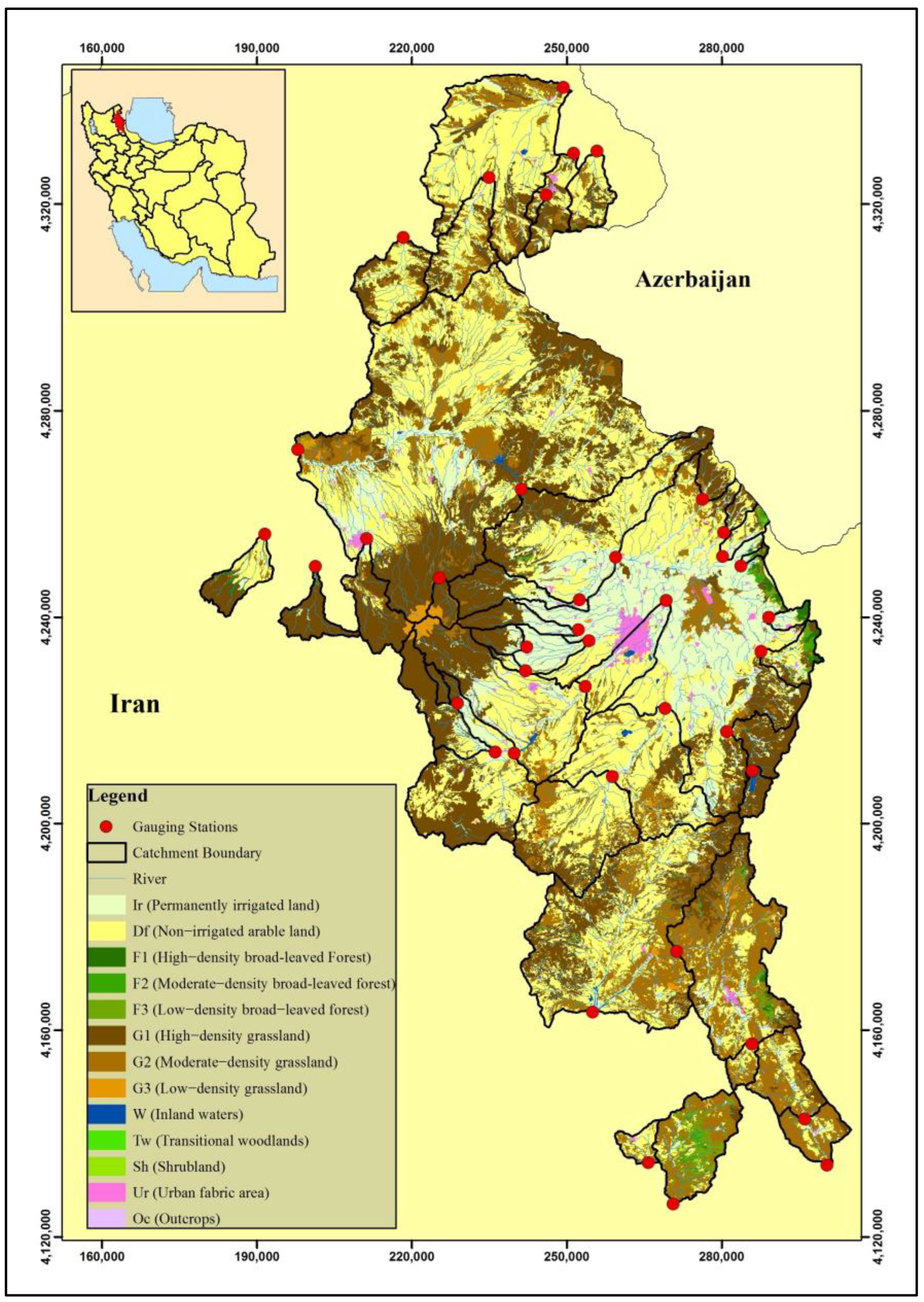
2.1. Study Area
2.2. Data Acquisition
2.3. Research Methodology
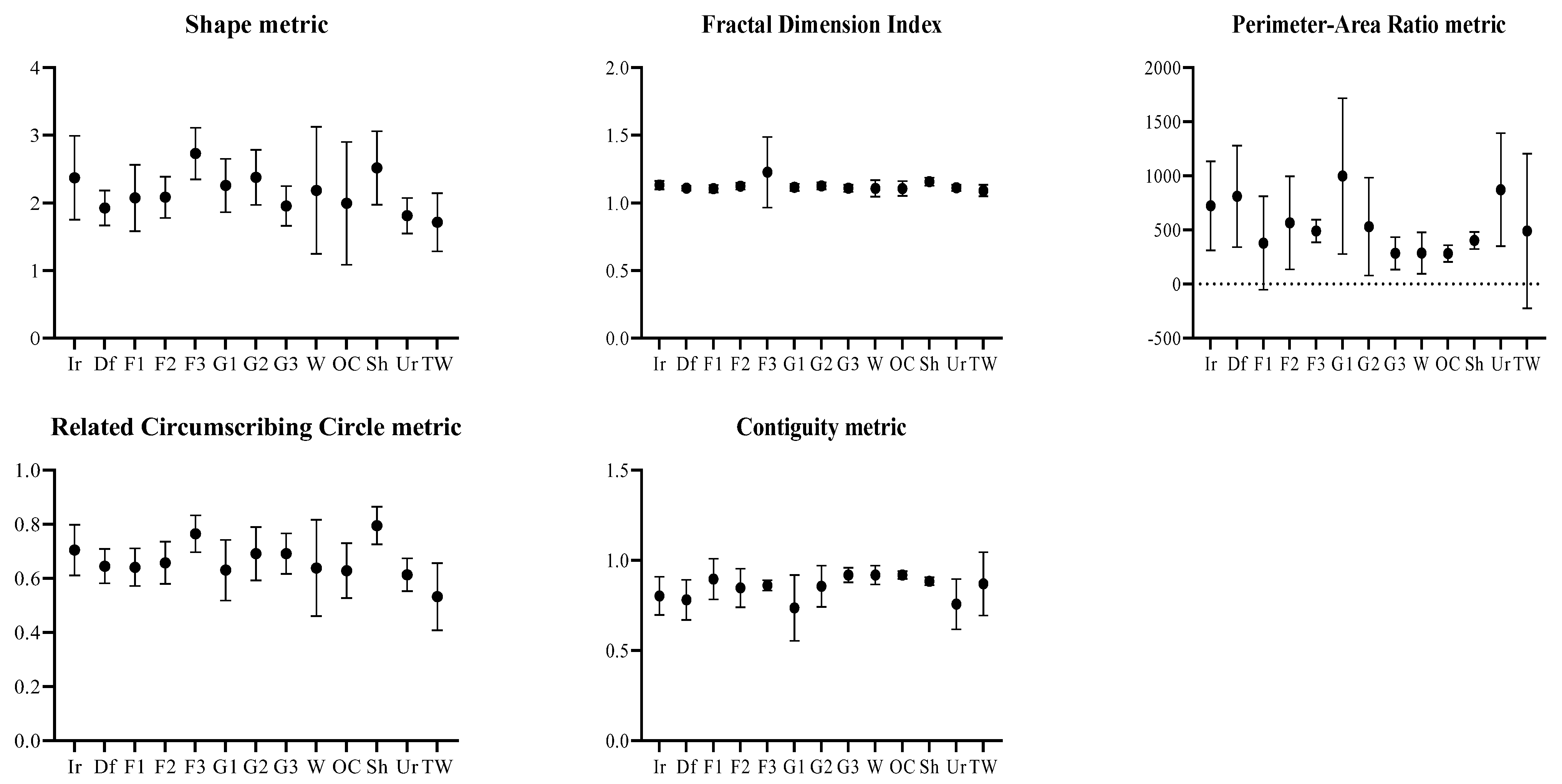
2.4. Calculation of Landscape Metrics
2.5. Statistical Calculations
2.6. Uncertainty Analysis
3. Results
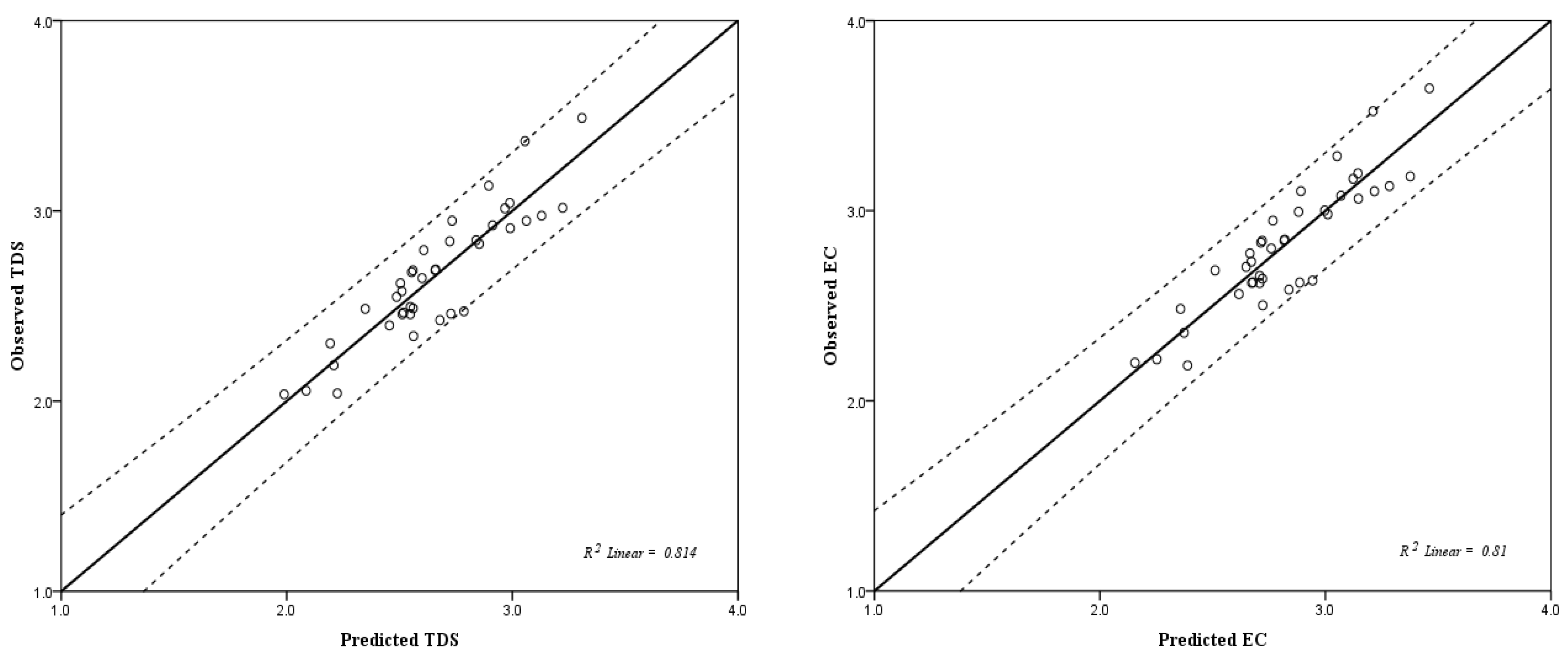
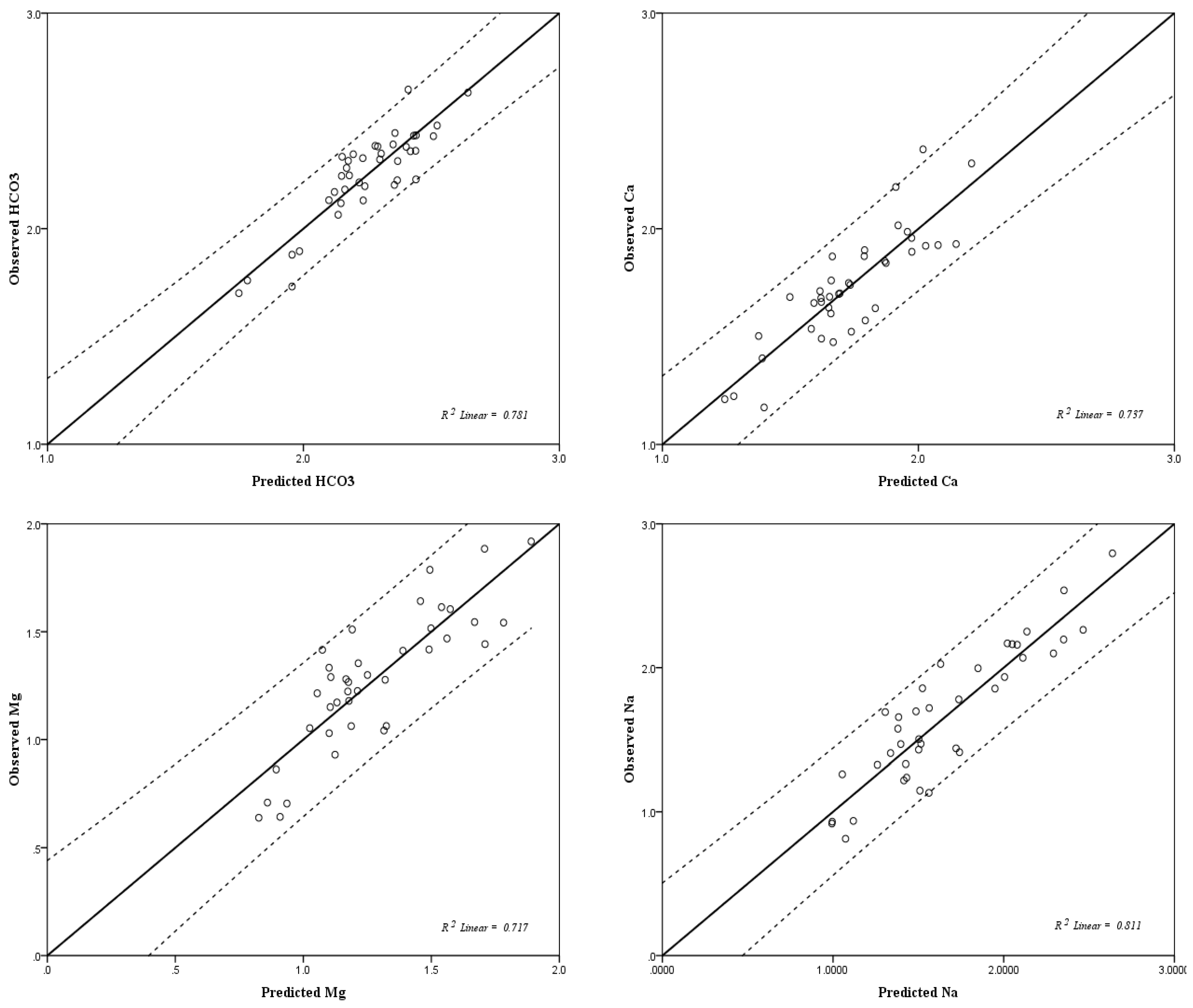
Modeling Results
- Q the discharge in m3·yr−1·ha−1,
- the shape index of the non-irrigated arable land,
- the fractal dimension index of the permanently irrigated land,
- the fractal dimension index of the high-density grassland,
- the fractal dimension index of the transitional woodlands, and
- stands for the contiguity index of the moderate-density grassland.
4. Discussion
5. Conclusions
Author Contributions
Funding
Institutional Review Board Statement
Informed Consent Statement
Data Availability Statement
Acknowledgments
Conflicts of Interest
References
- Lin, Y.-P.; Verburg, P.H.; Chang, C.-R.; Chen, H.-Y.; Chen, M.-H. Developing and comparing optimal and empirical land-use models for the development of an urbanized watershed forest in Taiwan. Landsc. Urban Plan. 2009, 92, 242–254. [Google Scholar] [CrossRef]
- Haidary, A.; Amiri, B.J.; Adamowski, J.; Fohrer, N.; Nakane, K. Assessing the impacts of four land use types on the water quality of wetlands in Japan. Water Resour. Manag. 2013, 27, 2217–2229. [Google Scholar] [CrossRef]
- Xie, Y.; Yu, X.; Ng, N.C.; Li, K.; Fang, L. Exploring the dynamic correlation of landscape composition and habitat fragmentation with surface water quality in the Shenzhen river and deep bay cross-border watershed, China. Ecol. Indic. 2018, 90, 231–246. [Google Scholar] [CrossRef]
- Oliveira, J.; Becegato, V.R.; Barcarolli, I.F.; Paulino, A.; Becegato, V. Environmental Characteristics and Water Quality of a Drainage Basin Impacted by Human Activities. Environ. Manag. Sustain. Dev. 2017, 6, 373. [Google Scholar] [CrossRef]
- Aronson, R.B.; Hilbun, N.L.; Bianchi, T.S.; Filley, T.R.; Mckee, B.A. Land use, water quality, and the history of coral assemblages at Bocas del Toro, Panamá. Mar. Ecol. Prog. Ser. 2014, 504, 159–170. [Google Scholar] [CrossRef]
- Tanaka, M.O.; de Souza, A.L.T.; Moschini, L.E.; de Oliveira, A.K. Influence of watershed land use and riparian characteristics on biological indicators of stream water quality in southeastern Brazil. Agric. Ecosyst. Environ. 2016, 216, 333–339. [Google Scholar] [CrossRef]
- Zhang, X.; Liu, Y.; Zhou, L. Correlation analysis between landscape metrics and water quality under multiple scales. Int. J. Environ. Res. Public Health 2018, 15, 1606. [Google Scholar] [CrossRef]
- Liu, Z.; Yang, H. The impacts of spatiotemporal landscape changes on Water quality in Shenzhen, China. Int. J. Environ. Res. Public Health 2018, 15, 1038. [Google Scholar] [CrossRef]
- Ongley, E.D.; Xiaolan, Z.; Tao, Y. Current status of agricultural and rural non-point source pollution assessment in China. Environ. Pollut. 2010, 158, 1159–1168. [Google Scholar] [CrossRef]
- Shi, P.; Zhang, Y.; Li, Z.; Li, P.; Xu, G. Influence of land use and land cover patterns on seasonal water quality at multi-spatial scales. Catena 2017, 151, 182–190. [Google Scholar] [CrossRef]
- Chen, J.; Lu, J. Effects of land use, topography and socio-economic factors on river water quality in a mountainous watershed with intensive agricultural production in East China. PLoS ONE 2014, 9, e102714. [Google Scholar] [CrossRef] [PubMed]
- Barrosl, M.; Rosman, P.; Telles, J. Water quality modelling in tidal wetlands considering flooding and drying processes. River Basin Manag. VII 2012, 172, 421. [Google Scholar]
- Liu, J.; Zhang, C.; Kou, L.; Zhou, Q. Effects of climate and land use changes on water resources in the Taoer river. Adv. Meteorol. 2017, 2017, 1031854. [Google Scholar] [CrossRef]
- Wan, R.; Cai, S.; Li, H.; Yang, G.; Li, Z.; Nie, X. Inferring land use and land cover impact on stream water quality using a Bayesian hierarchical modeling approach in the Xitiaoxi River Watershed, China. J. Environ. Manag. 2014, 133, 1–11. [Google Scholar] [CrossRef] [PubMed]
- Cuo, L. Land use/cover change impacts on hydrology in large river basins: A review. Terr. Water Cycle Clim. Chang. Nat. Hum.-Induc. Impacts 2016, 221, 103. [Google Scholar]
- Gikas, G.D.; Yiannakopoulou, T.; Tsihrintzis, V.A. Water quality trends in a coastal lagoon impacted by non-point source pollution after implementation of protective measures. Hydrobiologia 2006, 563, 385–406. [Google Scholar] [CrossRef]
- Boskidis, I.; Gikas, G.D.; Pisinaras, V.; Tsihrintzis, V.A. Spatial and temporal changes of water quality, and SWAT modeling of Vosvozis river basin, North Greece. J. Environ. Sci. Health Part A 2010, 45, 1421–1440. [Google Scholar] [CrossRef]
- Amiri, B.J.; Nakane, K. Modeling the relationship between land cover and river water quality in the Yamaguchi prefecture of Japan. J. Ecol. Environ. 2006, 29, 343–352. [Google Scholar] [CrossRef]
- Sun, R.; Chen, L.; Chen, W.; Ji, Y. Effect of land-use patterns on total nitrogen concentration in the upstream regions of the Haihe River Basin, China. Environ. Manag. 2013, 51, 45–58. [Google Scholar] [CrossRef]
- Gorgoglione, A.; Gregorio, J.; Rios, A.; Alonso, J.; Chreties, C.; Fossati, M. Influence of land use/land cover on surface-water quality of Santa Lucìa river, Uruguay. Sustainability 2020, 12, 4692. [Google Scholar] [CrossRef]
- Kang, J.-H.; Lee, S.W.; Cho, K.H.; Ki, S.J.; Cha, S.M.; Kim, J.H. Linking land-use type and stream water quality using spatial data of fecal indicator bacteria and heavy metals in the Yeongsan river basin. Water Res. 2010, 44, 4143–4157. [Google Scholar] [CrossRef] [PubMed]
- Lee, S.-W.; Hwang, S.-J.; Lee, S.-B.; Hwang, H.-S.; Sung, H.-C. Landscape ecological approach to the relationships of land use patterns in watersheds to water quality characteristics. Landsc. Urban Plan. 2009, 92, 80–89. [Google Scholar] [CrossRef]
- Seeboonruang, U. A statistical assessment of the impact of land uses on surface water quality indexes. J. Environ. Manag. 2012, 101, 134–142. [Google Scholar] [CrossRef] [PubMed]
- Mehaffey, M.H.; Nash, M.; Wade, T.; Ebert, D.; Jones, K.; Rager, A. Linking land cover and water quality in New York City’s water supply watersheds. Environ. Monit. Assess. 2005, 107, 29–44. [Google Scholar] [CrossRef] [PubMed]
- Ouyang, W.; Hao, F.-H.; Wang, X.-L. Regional non point source organic pollution modeling and critical area identification for watershed best environmental management. Water Air Soil Pollut. 2008, 187, 251–261. [Google Scholar] [CrossRef]
- Nakane, K.; Heydari, A. Sensitivity analysis of stream water quality and land cover linkage models using Monte Carlo method. Int. J. Environ. Res. 2010, 4, 121–130. [Google Scholar]
- Mishra, A.; Singh, R.; Singh, V.P. Evaluation of non-point source N and P loads in a small mixed land use land cover watershed. J. Water Resour. Prot. 2010, 2, 362. [Google Scholar] [CrossRef]
- Uriarte, M.; Yackulic, C.B.; Lim, Y.; Arce-Nazario, J.A. Influence of land use on water quality in a tropical landscape: A multi-scale analysis. Landsc. Ecol. 2011, 26, 1151. [Google Scholar] [CrossRef]
- Liu, Z.; Wang, Y.; Li, Z.; Peng, J. Impervious surface impact on water quality in the process of rapid urbanization in Shenzhen, China. Environ. Earth Sci. 2013, 68, 2365–2373. [Google Scholar] [CrossRef]
- Teixeira, Z.; Teixeira, H.; Marques, J.C. Systematic processes of land use/land cover change to identify relevant driving forces: Implications on water quality. Sci. Total Environ. 2014, 470, 1320–1335. [Google Scholar] [CrossRef]
- Basnyat, P.; Teeter, L.D.; Flynn, K.M.; Lockaby, B.G. Relationships between landscape characteristics and nonpoint source pollution inputs to coastal estuaries. Environ. Manag. 1999, 23, 539–549. [Google Scholar] [CrossRef] [PubMed]
- Bhaduri, B.; Harbor, J.; Engel, B.; Grove, M. Assessing watershed-scale, long-term hydrologic impacts of land-use change using a GIS-NPS model. Environ. Manag. 2000, 26, 643–658. [Google Scholar] [CrossRef] [PubMed]
- Uuemaa, E.; Roosaare, J.; Mander, Ü. Landscape metrics as indicators of river water quality at catchment scale. Hydrol. Res. 2007, 38, 125–138. [Google Scholar] [CrossRef]
- Wickham, J.; Riitters, K.; Wade, T.; Coulston, J. Temporal change in forest fragmentation at multiple scales. Landsc. Ecol. 2007, 22, 481–489. [Google Scholar] [CrossRef]
- Turner, R.E.; Rabalais, N.N. Linking landscape and water quality in the Mississippi River basin for 200 years. Bioscience 2003, 53, 563–572. [Google Scholar] [CrossRef]
- Amiri, B.J.; Nakane, K. Modeling the linkage between river water quality and landscape metrics in the Chugoku district of Japan. Water Resour. Manag. 2009, 23, 931–956. [Google Scholar] [CrossRef]
- Liu, W.; Zhang, Q.; Liu, G. Influences of watershed landscape composition and configuration on lake-water quality in the Yangtze River basin of China. Hydrol. Process. 2012, 26, 570–578. [Google Scholar] [CrossRef]
- Zhou, T.; Wu, J.; Peng, S. Assessing the effects of landscape pattern on river water quality at multiple scales: A case study of the Dongjiang River watershed, China. Ecol. Indic. 2012, 23, 166–175. [Google Scholar] [CrossRef]
- Shen, Z.; Hou, X.; Li, W.; Aini, G.; Chen, L.; Gong, Y. Impact of landscape pattern at multiple spatial scales on water quality: A case study in a typical urbanised watershed in China. Ecol. Indic. 2015, 48, 417–427. [Google Scholar] [CrossRef]
- Clément, F.; Ruiz, J.; Rodríguez, M.A.; Blais, D.; Campeau, S. Landscape diversity and forest edge density regulate stream water quality in agricultural catchments. Ecol. Indic. 2017, 72, 627–639. [Google Scholar] [CrossRef]
- Afed Ullah, K.; Jiang, J.; Wang, P. Land use impacts on surface water quality by statistical approaches. Glob. J. Environ. Sci. Manag. 2018, 4, 231–250. [Google Scholar]
- Li, S.; Yang, H.; Lacayo, M.; Liu, J.; Lei, G. Impacts of land-use and land-cover changes on water yield: A case study in Jing-Jin-Ji, China. Sustainability 2018, 10, 960. [Google Scholar] [CrossRef]
- Caja, C.; Ibunes, N.; Paril, J.; Reyes, A.; Nazareno, J.; Monjardin, C.; Uy, F. Effects of land cover changes to the quantity of water supply and hydrologic cycle using water balance models. In Proceedings of the Malaysian Technical University Conference on Engineering and Technology (MUCET 2017), Penang, Malaysia, 6–7 December 2017; p. 06004. [Google Scholar]
- Guzha, A.; Rufino, M.C.; Okoth, S.; Jacobs, S.; Nóbrega, R. Impacts of land use and land cover change on surface runoff, discharge and low flows: Evidence from East Africa. J. Hydrol. Reg. Stud. 2018, 15, 49–67. [Google Scholar] [CrossRef]
- Mpo, A. Ardabil Province Landuse Planning Manage Report; Management and Planning Organization: Ardabil, Iran, 2012. [Google Scholar]
- European Environment Agency. CORINE Land Cover Product User Manual (Version 1.0); European Environment Agency: Copenhagen, Denmark, 2021. [Google Scholar]
- Forman, R.; Gordon, M. Landscape Ecology; John Wiley: New York, NY, USA, 1986; Volume 619. [Google Scholar]
- Rutledge, D.T. Landscape indices as measures of the effects of fragmentation: Can pattern reflect process? DOC Sci. Intern. Ser. 2003, 98, 5–27. [Google Scholar]
- Turner, M.G.; Gardner, R.H.; O’neill, R.V.; O’Neill, R.V. Landscape Ecology in Theory and Practice; Springer: Amsterdam, The Netherlands, 2001; Volume 401. [Google Scholar]
- Mcgarigal, K.; Marks, B.J. Spatial Pattern Analysis Program for Quantifying Landscape Structure; Gen. Tech. Rep. PNW-GTR-351; US Department of Agriculture, Forest Service, Pacific Northwest Research Station: La Grande, OR, USA, 1995; pp. 1–122. [Google Scholar]
- Neter, J.; Kutner, M.H.; Nachtsheim, C.J.; Wasserman, W. Applied Linear Statistical Models; Irwin: Chicago, IL, USA, 1996; Volume 4. [Google Scholar]
- Chatterjee, S.; Hadi, A.S. Regression Analysis by Example; John Wiley & Sons: Hoboken, NJ, USA, 2015. [Google Scholar]
- Amiri, B.J.; Fohrer, N.; Cullmann, J.; Hörmann, G.; Müller, F.; Adamowski, J. Regionalization of tank model using landscape metrics of catchments. Water Resour. Manag. 2016, 30, 5065–5085. [Google Scholar] [CrossRef]
- Dawson, C.W.; Abrahart, R.J.; See, L.M. HydroTest: A web-based toolbox of evaluation metrics for the standardised assessment of hydrological forecasts. Environ. Model. Softw. 2007, 22, 1034–1052. [Google Scholar] [CrossRef]
- Wagener, T.; Montanari, A. Convergence of approaches toward reducing uncertainty in predictions in ungauged basins. Water Resour. Res. 2011, 47. [Google Scholar] [CrossRef]
- Convertino, M.; Muñoz-Carpena, R.; Chu-Agor, M.L.; Kiker, G.A.; Linkov, I. Untangling drivers of species distributions: Global sensitivity and uncertainty analyses of MaxEnt. Environ. Model. Softw. 2014, 51, 296–309. [Google Scholar] [CrossRef]
- Amiri, B.; Sudheer, K.; Fohrer, N. Linkage between in-stream total phosphorus and land cover in Chugoku district, Japan: An ANN approach. J. Hydrol. Hydromech. 2012, 60, 33–44. [Google Scholar] [CrossRef]
- Amiri, B.J.; Gao, J.; Fohrer, N.; Adamowski, J.; Huang, J. Examining lag time using the landscape, pedoscape and lithoscape metrics of catchments. Ecol. Indic. 2019, 105, 36–46. [Google Scholar] [CrossRef]
- Rykiel, E.J., Jr. Testing ecological models: The meaning of validation. Ecol. Model. 1996, 90, 229–244. [Google Scholar] [CrossRef]
- Arora, J. Introduction to Optimum Design; Elsevier: Amsterdam, The Netherlands, 2004. [Google Scholar]
- Bu, H.; Meng, W.; Zhang, Y.; Wan, J. Relationships between land use patterns and water quality in the Taizi River basin, China. Ecol. Indic. 2014, 41, 187–197. [Google Scholar] [CrossRef]
- Xiao, H.; Ji, W. Relating landscape characteristics to non-point source pollution in mine waste-located watersheds using geospatial techniques. J. Environ. Manag. 2007, 82, 111–119. [Google Scholar] [CrossRef] [PubMed]
- Johnson, L.; Richards, C.; Host, G.; Arthur, J. Landscape influences on water chemistry in Midwestern stream ecosystems. Freshw. Biol. 1997, 37, 193–208. [Google Scholar] [CrossRef]
- Scown, M.W.; Flotemersch, J.E.; Spanbauer, T.L.; Eason, T.; Garmestani, A.; Chaffin, B.C. People and water: Exploring the social-ecological condition of watersheds of the United States. Elem. Sci. Anthr. 2017, 5, 64. [Google Scholar] [CrossRef]
- Hazbavi, Z.; Baartman, J.E.; Nunes, J.P.; Keesstra, S.D.; Sadeghi, S.H. Changeability of reliability, resilience and vulnerability indicators with respect to drought patterns. Ecol. Indic. 2018, 87, 196–208. [Google Scholar] [CrossRef]
- McGarigal, K. Landscape Pattern Metrics; Wiley StatsRef: Hoboken, NJ, USA, 2014. [Google Scholar]
- Tong, S.T.; Chen, W. Modeling the relationship between land use and surface water quality. J. Environ. Manag. 2002, 66, 377–393. [Google Scholar] [CrossRef]
- Uuemaa, E.; Roosaare, J.; Oja, T.; Mander, Ü. Analysing the spatial structure of the Estonian landscapes: Which landscape metrics are the most suitable for comparing different landscapes? Est. J. Ecol. 2011, 60, 70. [Google Scholar] [CrossRef]
- Amiri, B.J.; Gao, J.; Fohrer, N.; Adamowski, J. Regionalizing time of concentration using landscape structural patterns of catchments. J. Hydrol. Hydromech. 2019, 67, 135–142. [Google Scholar] [CrossRef]
- Sullivan, A.; Ternan, J.; Williams, A. Land use change and hydrological response in the Camel catchment, Cornwall. Appl. Geogr. 2004, 24, 119–137. [Google Scholar] [CrossRef]
- Kakehmami, A.; Ghorbani, A.; Moameri, M.; Ghafari, S. Evaluation of land use changes in Ardabil province using satellite image processing. Iran. J. Range Desert Res. 2021, 28, 537–550. [Google Scholar]
- Gyenizse, P.; Bognár, Z.; Czigány, S.; Elekes, T. Landscape shape index, as a potencial indicator of urban development in Hungary. Acta Geogr. Debrecina Landsc. Environ. 2014, 8, 78–88. [Google Scholar]
- Leitao, A.B.; Ahern, J. Applying landscape ecological concepts and metrics in sustainable landscape planning. Landsc. Urban Plan. 2002, 59, 65–93. [Google Scholar] [CrossRef]

| Name | Description | Formula |
|---|---|---|
| Shape Index | For a square-shaped patch, the value of the index is equal to 0, but for an irregular shape-patch, it is ∞ [47]. | |
| Fractal Dimension Index | The index ranges between 1 for a regular (square) patch and 2 for an irregular (convoluted) patch [48,49]. | |
| Perimeter–Area Ratio | The farther the ratio is from 1, the more the patch deviates from the isodiametric shape [48,50]. | |
| Related Circumscribing Circle | It varies from 0 for a convoluted patch to 1 for an elongated patch [49]. | |
| Contiguity Index | The value of metric varies between 0 for a one-pixel patch and 1 for a connected patch [50]. |
| Type | Metric | Equation | Range |
|---|---|---|---|
| Relative Error Models | Mean Relative Error (MRE) | 0–∞ | |
| Mean Absolute Relative Error (MARE) | 0–∞ | ||
| Relative Absolute Error (RAE) | 0–∞ | ||
| Model Efficiency | Coefficient of Determination (r2) | 0–1 | |
| Consistency Index (IA) | 0–∞ | ||
| Coefficient of Efficiency (CE) | 0–∞ | ||
| Absolute Error Models | Root Mean Square Error (RMSE) | 0–∞ | |
| Mean Error (ME) | 0–∞ | ||
| Mean Absolute Error (MAE) | 0–∞ |
| Model | Coefficients | Collinearity Statistics | |||||||
|---|---|---|---|---|---|---|---|---|---|
| Model | Variable | B | Std. Error | Beta | r2 | t | Sig. | Tolerance | VIF |
| TDS | Constant | 3.849 | 0.177 | 0. 81 | 21.730 | 0.000 | |||
| Discharge | −0.499 | 0.044 | −0.829 | −11.226 | 0.000 | 0.947 | 1.056 | ||
| Shape Df | 0.975 | 0.337 | 0.214 | 2.895 | 0.006 | 0.947 | 1.056 | ||
| EC | Constant | 3.996 | 0.178 | 0.81 | 22.494 | 0.000 | |||
| Discharge | −0.493 | 0.045 | −0.827 | −11.069 | 0.000 | 0.947 | 1.056 | ||
| Shape Df | 0.962 | 0.338 | 0.213 | 2.846 | 0.007 | 0.947 | 1.056 | ||
| HCO3 | Constant | 2.921 | 0.146 | 0.78 | 20.074 | 0.000 | |||
| Discharge | −0.252 | 0.033 | −0.651 | −7.707 | 0.000 | 0.904 | 1.106 | ||
| FRAC Ir | 7.101 | 1.314 | 0.467 | 5.402 | 0.000 | 0.863 | 1.158 | ||
| FRAC G1 | −7.171 | 1.513 | −0.420 | −4.740 | 0.000 | 0.822 | 1.217 | ||
| FRAC TW | 2.874 | 1.080 | 0.225 | 2.662 | 0.012 | 0.903 | 1.108 | ||
| Ca | Constant | 2.572 | 0.165 | 0.74 | 15.553 | 0.000 | |||
| Discharge | −0.366 | 0.041 | −0.775 | −8.818 | 0.000 | 0.947 | 1.056 | ||
| Shape Df | 0.829 | 0.315 | 0.232 | 2.636 | 0.012 | 0.947 | 1.056 | ||
| Mg | Constant | 2.630 | 0.149 | 0.71 | 17.648 | 0.000 | |||
| Discharge | −0.485 | 0.051 | −0.857 | −9.535 | 0.000 | 0.973 | 1.027 | ||
| CONTIG G2 | −0.877 | 0.409 | −0.193 | −2.144 | 0.039 | 0.973 | 1.027 | ||
| Na | Constant | 3.801 | 0.182 | 0.81 | 20.907 | 0.000 | |||
| Discharge | −0.768 | 0.062 | −0.909 | −12.390 | 0.000 | 0.973 | 1.027 | ||
| CONTIG G2 | −1.540 | 0.499 | −0.227 | −3.086 | 0.004 | 0.973 | 1.027 | ||
| Model | Relative Error Model | Model Efficiency | Absolute Error Model | ||||||
|---|---|---|---|---|---|---|---|---|---|
| MRE | MARE | RAE | IA | CE | r2 | RMSE | ME | MAE | |
| TDS | −0.02 | 0.04 | 0.54 | 0.93 | 0.78 | 0.82 | 0.15 | −0.04 | 0.1 |
| EC | −0.02 | 0.03 | 0.54 | 0.93 | 0.78 | 0.82 | 0.14 | −0.04 | 0.1 |
| HCO3 | 0.01 | 0.03 | 0.7 | 0.91 | 0.68 | 0.71 | 0.09 | 0.01 | 0.07 |
| Ca | −0.03 | 0.05 | 0.59 | 0.93 | 0.76 | 0.81 | 0.11 | −0.04 | 0.08 |
| Mg | −0.03 | 0.08 | 0.62 | 0.92 | 0.71 | 0.74 | 0.14 | −0.03 | 0.1 |
| Na | −0.01 | 0.12 | 0.71 | 0.91 | 0.7 | 0.7 | 0.24 | 0.01 | 0.18 |
| Variable | Model Variable | Statistical | Kolmogorov Smirnov | Statistical | ||
|---|---|---|---|---|---|---|
| Distribution | Statistics | p-Value | Variables | |||
| TDS | A prior statistics | Discharge | Wakeby | 0.08914 | 0.88883 | α = 1531 β = 0.19338 γ = 40.077 δ = 0.93225 ζ = −46.396 |
| Shape Df | Weibull | 0.0936 | 0.85262 | α = 8.3969 β = 2.0382 γ = 0 | ||
| Posterior statistics | Yobs. | Lognormal (3P) | 0.08334 | 0.92856 | α = 0.88486 μ = 5.9758 γ = 45.878 | |
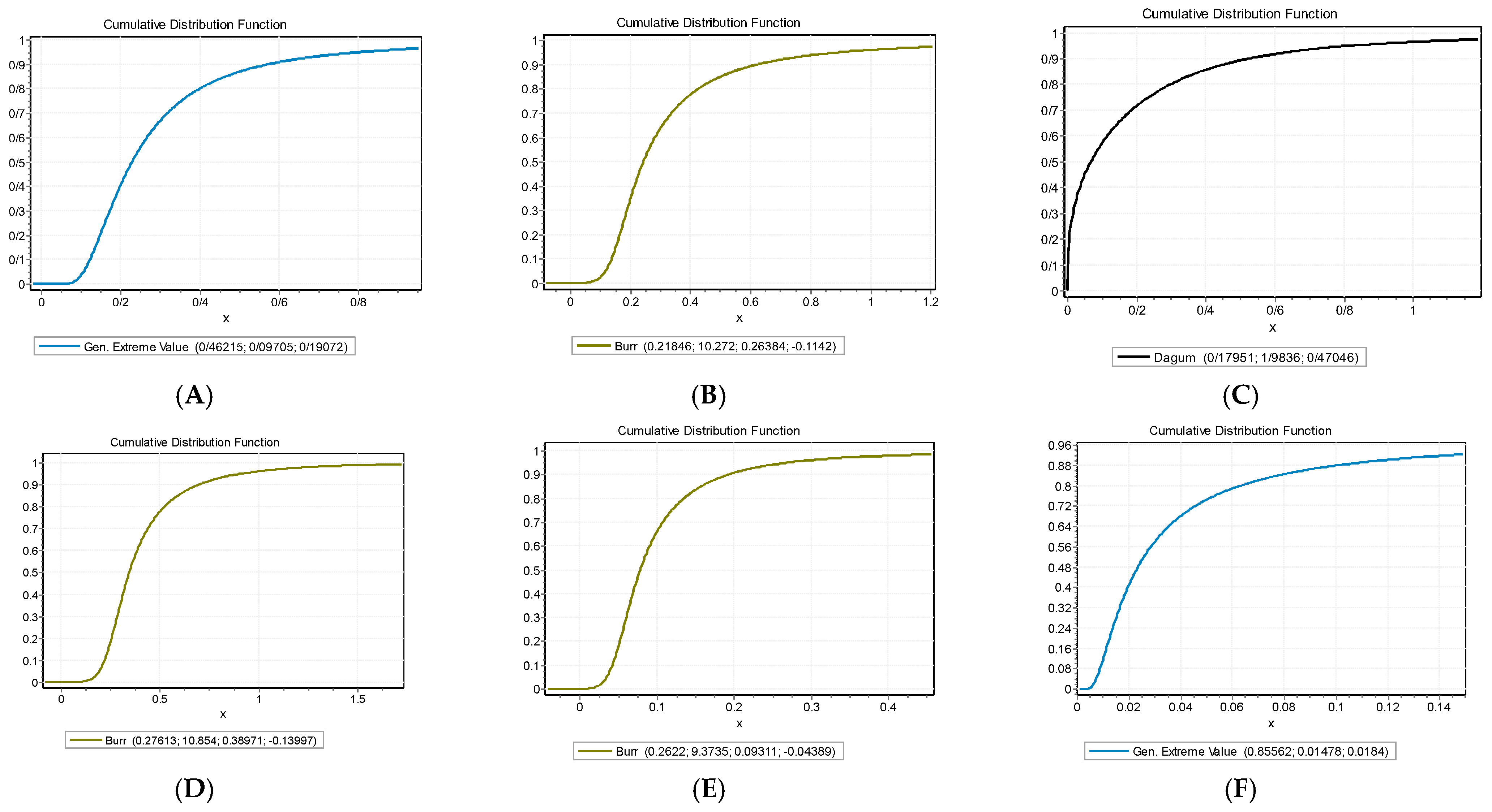
| YSim. | Gen.Extreme value | 0.05299 | 0.99964 | κ = 0.46215 σ = 0.09705 μ = 0.19072 | ||
| EC | A prior statistics | Discharge | Wakeby | 0.08914 | 0.88883 | α = 1531 β = 0.19338 γ = 40.077 δ = 0.93225 ζ = −46.396 |
| Shape Df | Weibull | 0.0936 | 0.85262 | α = 8.3969 β = 2.0382 γ = 0 | ||
| Posterior statistics | Yobs. | Frechet | 0.06909 | 0.98592 | α = 2.3788 β = 804.97 γ = −305.53 | |
| YSim. | Burr (4P) | 0.00645 | 0.5588 | κ= 0.20543 α = 11.513 β = 0.28681 γ = −0.1404 | ||
| HCO3 | A prior statistics | Discharge | Wakeby | 0.08914 | 0.88883 | α = 1531 β = 0.19338 γ = 40.077 δ = 0.93225 ζ = −46.396 |
| FRAC Ir | Cauchy | 0.07862 | 0.9539 | σ = 0.01357 μ = 1.1324 | ||
| FRAC G1 | Dagum | 0.09029 | 0.87996 | κ = 0.15021 α = 291.26 β = 1.1397 γ = 0 | ||
| FRAC PF | Uniform | 0.4395 | 2.9227 × 10⁻⁷ | α = −0.55009 β = 0.99785 | ||
| Yobs. | Hypersecant | 0.0765 | 0.9632 | α = 85.625 μ = 196.75 | ||
| Posterior statistics | YSim. | Dagum | 0.03255 | 4.8608 × 10⁻⁹ | κ = 0.17951 α = 1.9836 β = 0.47046 γ = 0 | |
| Ca | A prior statistics | Discharge | Wakeby | 0.08914 | 0.88883 | α = 1531 β = 0.19338 γ = 40.077 δ = 0.93225 ζ = −46.396 |
| Shape Df | Weibull | 0.0936 | 0.85262 | α = 8.3969 β = 2.0382 γ = 0 | ||
| Yobs. | Frechet | 0.0661 | 0.99133 | α = 4.4327 β = 107.45 γ = −63.329 | ||
| Posterior statistics | YSim. | Burr (4P) | 0.00833 | 0.26122 | κ = 0.27613 α = 10.854 β = 0.3897 γ = −0.13997 | |
| Mg | A prior statistics | Discharge | Wakeby | 0.08914 | 0.88883 | α = 1531 β = 0.19338 γ = 40.077 δ = 0.93225 ζ = −46.396 |
| Contig G2 | Gen.Logistic | 0.07469 | 0.9701 | κ = −0.52828 α = 0.05592 μ = 0.88399 | ||
| Yobs. | Gen.Extreme value | 0.05299 | 0.99964 | κ = 0.21042 σ = 10.558 μ = 15.286 | ||
| Posterior statistics | YSim. | Burr (4P) | 0.00806 | 0.30806 | κ = 0.27851 α = 8.8673 β = 0.09248 γ = −0.0424 | |
| Na | A prior statistics | Discharge | Wakeby | 0.08914 | 0.88883 | α = 1531 β = 0.19338 g = 40.077 δ = 0.93225 ζ = −46.396 |
| Contig G2 | Gen.Logistic | 0.07469 | 0.9701 | κ = −0.52828 α = 0.05592 μ = 0.88399 | ||
| Yobs. | Fatigue life (3P) | 0.07012 | 0.9836 | α = 1.4239 β = 39.534 γ = 3.4162 | ||
| Posterior statistics | YSim. | Gen.Extreme value | 0.00964 | 0.1372 | κ = 0.85562 σ = 0.01478 μ = 0.0184 | |
Disclaimer/Publisher’s Note: The statements, opinions and data contained in all publications are solely those of the individual author(s) and contributor(s) and not of MDPI and/or the editor(s). MDPI and/or the editor(s) disclaim responsibility for any injury to people or property resulting from any ideas, methods, instructions or products referred to in the content. |
© 2023 by the authors. Licensee MDPI, Basel, Switzerland. This article is an open access article distributed under the terms and conditions of the Creative Commons Attribution (CC BY) license (https://creativecommons.org/licenses/by/4.0/).
Share and Cite
Aalipour, M.; Wu, N.; Fohrer, N.; Kianpoor Kalkhajeh, Y.; Jabbarian Amiri, B. Examining the Influence of Landscape Patch Shapes on River Water Quality. Land 2023, 12, 1011. https://doi.org/10.3390/land12051011
Aalipour M, Wu N, Fohrer N, Kianpoor Kalkhajeh Y, Jabbarian Amiri B. Examining the Influence of Landscape Patch Shapes on River Water Quality. Land. 2023; 12(5):1011. https://doi.org/10.3390/land12051011
Chicago/Turabian StyleAalipour, Mehdi, Naicheng Wu, Nicola Fohrer, Yusef Kianpoor Kalkhajeh, and Bahman Jabbarian Amiri. 2023. "Examining the Influence of Landscape Patch Shapes on River Water Quality" Land 12, no. 5: 1011. https://doi.org/10.3390/land12051011