Abstract
China’s urbanisation process is unique compared to that of other developed economies in that while the rural population is migrating to the cities in large numbers, the area of rural homestead use also continues to increase. This research uses macro data and a threshold model to further analyse this phenomenon of “farmers leaving while rural homestead increasing”. Specifically, we focus on the mechanisms of action, development patterns and regional differences in the impact of the rate of rural–urban migration (RRUM) on the rate of increase in the area of rural homesteads (IARH), and discuss the spatial spillover effects of the impact between the two. The results of the research show that: (1) There is an “inverted U-shaped” double threshold effect on the impact of RRUM on IARH. (2) Rural population density and regional urban–rural income disparity are used as threshold variables, respectively, resulting in a sudden change in the relationship between RRUM and IARH. (3) The threshold effect of RRUM on IARH mainly exists in the central and western regions, non-minority nationality areas, non-provincial capital cities and non-resource-based cities. (4) The RRUM can not only directly affect the local IARH, but also indirectly affect the surrounding areas through spatial spillover effects. Our research provides critical insights for policy makers on the reform of the rural homestead system and urbanisation development strategies in different regions.
1. Introduction
Since reform and opening up, China’s ‘economic growth miracle’ and rapid urbanisation have produced a historic structural transformation [1,2]. In the process of rapid economic change, a large number of rural migrant workers have moved to the cities and have gradually taken up permanent residence there [3]. However, this process of migration has also led to an increase in the use of rural homesteads. The phenomenon of ‘farmers leaving while rural homestead increasing’ in the countryside has become one of the key features of China’s urbanisation. Roback [4] suggested that young, skilled people will move to the cities and relocate to the big cities, leaving the countryside behind. However, as housing rents (costs) rise, a growing number of international scholars have pointed out that rising house prices seriously discourage mobility and have a negative effect on urbanisation [5]. Bjerke and Mellander [6] indicated that, in Sweden, housing prices inhibit migration to high-cost areas and further facilitate the return of urban to rural populations. Ji [7] argued that under the pressure of high housing prices and the dualistic urban–rural division of the household registration system, many rural migrant workers choose to return to their home villages to build farmhouses after earning money in the cities of their inflow. This is the case for the construction of farmhouses in villages. This phenomenon of “building new houses without demolishing the old ones” within villages is a recurring one, and the lack of scientific village planning has led to a continuous expansion of rural settlements. This particular relationship between farmers and the rural land has attracted the interest of scholars [8,9].
According to data from the Seventh National Population Census of China, it can be seen that the migrant population has increased by 69.73% compared to 2010, and the 2021 Migrant Workers Monitoring Survey Report shows that there are also over 130 million migrant workers living in cities and towns. All of the above figures show that the number of rural–urban migrants continues to grow, and that many have chosen to settle in cities during their mobility. However, the fact is that the area of rural homestead use has increased in parallel with the rural exodus [10]. Studies on the impact of rural migration on rural land use have focused on the impact of rural exodus on the use of contracted land, such as the loss of rural populations, resulting in the abandonment of arable land and the reduction in arable land area. The current literature is less concerned with the use of rural homesteads, which is important for residential security. Some studies point to a sustained increase in the size of the homestead area in the rural exodus, but whether this increase is sustained and what the regional differences are has not been explored. Why do rural people still need rural homesteads to provide security for residential functions when they are moving to and living in cities in large numbers? Based on this question, this research argues that exploring the relationships, patterns and regional differences between rural–urban migration and rural homestead use in China can provide a better understanding of China’s particular pattern of economic structural change.
Based on the above analysis, the central issue that this research wants to focus on is how the process of the rural–urban migration of Chinese farmers has affected the use of rural homesteads. Specifically, we aim to examine the following issues: Firstly, why does the area of rural homestead in China continue to increase despite the continuous migration of the rural population to the cities? Secondly, is this increase a phased phenomenon, and will it continue? What factors may affect and change this phenomenon? Thirdly, does the phenomenon of “farmers leaving while rural homestead increasing” show the same pattern in different regions in China? To explore these issues, we used panel data for urban areas from 2009 to 2016 to analyse the non-linear relationship between the RRUM and the IARH through a threshold model. The inverted U-shaped relationship between the RRUM and the IARH was then further explored using rural population density and the urban–rural income gap as threshold variables. We then used multi-level urban indicators to analyse the heterogeneous effect of the RRUM on the IARH, and finally discussed the spatial spillover effects of the two using a spatial Durbin fixed effects model.
In terms of theoretical significance, this study can enrich the research findings on labour migration based on the rural–urban context in China from a land perspective, so as to better understand the particular phenomenon in the transformation of China’s urban–rural structure. In practical terms, this study further analyses the real demand of rural migrations for rural land based on this special relationship between people and land, and thus promotes the New Urbanization Strategy with people at its core. Understanding the development patterns, regional differences and spatial spillover effects of the relationship between rural migrations and land can help to better provide policy references for the ongoing reform of China’s rural homestead system. This research tries to make innovations from the following points. Firstly, the research perspective is innovative. We used the relationship between the RRUM and the IARH to understand the inseparable relationship between farmers and land in China’s economic structural transformation, and further dissected the development pattern of this human–land dependency relationship, enriching the study of the impact of rural–urban migration on rural land use in China. Secondly, the models and methods used in this paper allowed for a more accurate analysis of phase changes. We used a threshold model instead of other linear regression models, which could accurately identify that this human–land dependency relationship is not a single linear increase, but an inverted U-shaped pattern of increase followed by decrease. At the same time, the use of the threshold model can effectively identify the factors that cause sudden changes in the human–land dependency relationship, and can thus more accurately reflect the development patterns of rural exodus and rural homestead use. Thirdly, the classification of regional differences is innovative. Based on China’s own institutional and humanistic background, we discussed the relationship between RRUM and the IARH in different regions, not only considering the economic development of the region, but also using variables such as minority nationality and regional resource endowment to analyse regional differences based on different indicator classifications.
The remainder of the paper is organized as follows. In Section 2 we review the literature on the impact of rural–urban mobility on the behaviour of farmers and provide a theoretical analysis. Section 3 presents the data sources, variable settings and models. Section 4 presents the empirical analysis and results. In Section 5 we conduct an analysis of urban heterogeneity and mechanisms. In Section 6 we further investigate the spatial spillover effects. Finally, we discuss the conclusions and make relevant policy recommendations.
2. Literature Review and Theoretical Analysis
2.1. Research on Rural–Urban Mobility and Land Use Relations
The process of structural transformation is accompanied by a process of ‘de-agriculturalisation’, a gradual transition from an ‘agrarian civilisation’ to an ‘urban and industrial civilisation’ and the transfer of surplus rural labour to the cities [11,12]. In the study of rural–urban mobility, scholars have conducted a large number of studies on the development pattern of agricultural population transfer, the connotations and influencing factors of the citizenship of rural populations and the characteristics of mobile populations, respectively [13,14,15]. As related research progresses, more literature has focused on the uneven development of urbanisation due to the dualistic land system between urban and rural areas [16]. In a joint analysis of the land and labour factor markets, scholars have found a correlation between rural–urban mobility decisions of famers and their landholdings [17]. Currently, the effects of rural–urban migration on rural poverty rates [18], land use structure [19], rural consumption [20] and agro-ecological efficiency [21] have been widely discussed by many scholars.
For agricultural land, He [22] indicated that the process of rural–urban migration is likely to result in the abandonment of arable land, and that rural migrants who move to cities are more likely to transfer their land to friends and relatives or to large farmers in a market-based manner in order to avoid idle farmland. Meng [23] found that under the existing land use system, rural–urban migration leads to a mismatch of rural homestead resources within villages, further resulting in idle and wasteful rural homestead. In the discussion of the relationship between rural–urban migration and rural homestead use, Zhang [24] found that nearly half of migrant workers choose to return to their hometowns to build farm houses, based on micro-survey data. Tan et al. [25] argued that the transfer of employment of surplus rural labour promotes their investment in building houses in their hometowns. Niu [26] indicated that agricultural shifters’ construction of homesteads in their home villages has become one of their important consumption investments. These studies used the individual characteristics of farmers as a starting point to examine the impact on investment in farmhouse construction, but lacked a macro perspective on the overall or phased impact of the trend of continuous rural–urban migration on the use of rural homesteads.
2.2. Theoretical Analysis
Studies of urban–rural migration in different countries have shown that migrants’ decisions are often influenced by both the home city and the destination city [27]. In China’s dualistic urban–rural system, migrants show a stronger ‘linkage’ to their rural homestead in their rural–urban migration [28]. This is particularly evident in the rapid urbanisation of China, where the rural household registration population is declining, but at the same time the area of rural homesteads is still increasing. The impact of this rural–urban migration on the use of rural homesteads may stem from the following aspects. (1) Income effects: when wage incomes in the industrial sector are higher than those in the agricultural sector, surplus rural labour will move to the cities, a process that promotes economic growth and higher income levels for farmers, which in turn promotes higher levels of consumption [29,30]. The rise in the income of migrant workers lays the material basis for rural migrants to return to their hometowns to apply for rural homesteads and build new farmhouses [31]. Therefore, migrant workers are likely to return to their hometowns to renovate, expand or build new homesteads to improve the quality of family life. (2) Risk aversion: Due to the existence of the dualistic system between urban and rural areas in China, many rural–urban migrant workers are in a “semi-urbanised state” [32]. Due to the household registration system, the cost of living, the risk of unemployment and the cost of urban housing, it is difficult for rural–urban migrants to settle in their place of inflow or to enjoy the same public services as local urban residents [33]. In addition, scholars point out that the stability of property rights in farmers’ minds is higher for homesteads than for contracted land [34]. This is mainly due to the fact that the location of each family’s contracted land has had the potential to be adjusted in the past decades in some areas, but rural homesteads are generally not easily changed in terms of tenure. As a result, rural–urban migrants often see their rural homesteads as providing family security for unemployment and old age. (3) Potential benefits: As rural homesteads have welfare protection attributes, members of collective economic organisations in villages can apply for new rural homestead free of charge when they meet the conditions, and under the stimulus of egalitarianism farmers are prone to a “first-come-first-served, more-come-more” mentality to keep increasing the area of rural homesteads [35,36]. With the gradual advancement of the pilot reform of the homestead system, the asset value of homesteads has gradually emerged in many areas. Although there is no legal and clear market for trading, the potential income from renting and selling, and the potential compensation for land acquisition and demolition, have also increased the incentive for migrant workers to return to their hometowns to build new rural homesteads [37]. (4) Signal theory: rural homesteads can be used as a bulk investment item to satisfy villagers’ psychology of showing off and comparing within the village, releasing wealth signals [38]. They can also serve as a symbol of family assets and provide a good credit guarantee for children’s marriage contracts, etc. By building or expanding farmhouses, they can increase their wealth and personal status within the village, and even increase their chances of political participation at the grassroots level. Therefore, most rural–urban migrants show a tendency to want to expand their homesteads and repair their farmhouse when they return home after working in the inflow cities [39]. In general, the tendency of rural migrants to build or expand their homesteads is influenced by both their home village and the city where they are moving to (as shown in Figure 1).
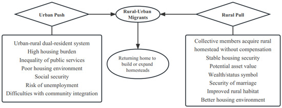
Figure 1.
Analysis of the driving forces of rural migrants’ homestead expansion based on push-pull theory.
2.3. Research Hypothesis
Although the migration of rural labour to the cities has shown a certain amount of “rural house building fever”, this phenomenon is unlikely to last forever. As the rural exodus continues to increase, some villages are becoming “hollow villages”. Further, some cities are even becoming ‘outflow’ or ‘shrinkage’ cities, with the exodus of people and the migration of rural families [40]. In these areas, there is considerable scope for improving the living conditions, infrastructure and public services of the villages, but due to the massive labour exodus and the relatively high cost of infrastructure, many of the families that have migrated out of the area do not choose to return. Therefore, when the outflow of population reaches a certain level, it will be difficult to attract a large number of rural–urban migrants to return to their hometowns, and the incentive to apply for rural homesteads and build farmhouses will disappear. Based on the above analysis, this chapter proposes Hypothesis 1.
H1:
The effect of the RRUM on the IARH shows a positive and then negative inverted U-shaped relationship.
In addition, factors such as socio-economics and physical geography may also influence the relationship between rural exodus and the use of rural homesteads. In terms of socio-economic attributes, the urban–rural income gap can, to a certain extent, measure whether the economic development of a region is balanced between urban and rural areas. Many scholars have pointed out that the urban–rural income gap has a dampening effect on consumption, and that farmers in areas with a large income gap tend to “move up the social ladder” and flee their villages for the cities [41,42]. At the same time, the regional urban–rural income gap will also affect farmers’ investment expectations in land, as a large urban–rural income gap often implies poorer rural living conditions and infrastructure, thus discouraging farmers from building or expanding their homesteads. Therefore, when the urban–rural income gap is within a reasonable range, the rural exodus increases incomes, thus increasing the likelihood of returning to the countryside to build new homesteads. That is, the RRUM reflects a promotional effect on the IARH when the urban–rural income gap is small (Left half of Figure 2a).
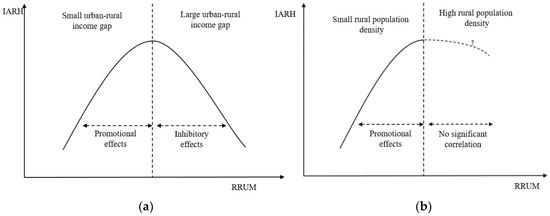
Figure 2.
Mechanistic diagram of the action of the threshold model when gap and density are used as threshold variables, respectively. (a) Relationship between RRUM and IARH for urban-rural income as a threshold variable. (b) Relationship between RRUM and IARH for rural population density as a threshold variable.
However, once the income gap between urban and rural areas exceeds a reasonable range, the area will lose a certain degree of “attraction” for the rural exodus, reducing the incentive for migrant workers to return to their hometowns. At this point, the stimulating effect of rural–urban migration on the increase in the area of rural homesteads will be offset, or even reverse, as shown by a gradual decrease in the IARH. At this time, RRUM manifests an inhibitory effect on IARH (right half of Figure 2a). Thus, the relationship between RRUM and IARH has an overall inverted U-shape under the influence of the urban–rural income gap, The mechanism of which is shown in Figure 2a. Therefore, we propose Hypothesis 2.
H2:
The relationship between the RRUM and the IARH is influenced by the regional urban–rural income gap, and when the regional urban–rural income gap reaches a certain threshold, the relationship between the two will change from positive to negative abruptly.
In terms of geographical factors, rural population density can, to a certain extent, reflect the relationship between people and land and the supply and demand of rural land [43]. Lower densities mean that the rural population in the area is small or that the area is sparsely populated, such as in mountainous or hilly areas. However, denser areas often lack back-up resources for rural homesteads, and even new approvals for farmhousing have been halted [44]. Therefore, when rural population density is within a certain range, rural population outflow may stimulate new rural homestead construction after returning to the countryside. That is, the RRUM reflects a promotional effect on the IARH when the rural population density is small (left half of Figure 2b). However, once population density exceeds a reasonable interval, it may limit the maximum amount of the new rural homestead area. At this point, the objective conditions of geography will prevent an unlimited increase in the number of homesteads. Therefore, there may not be any significant correlation between RRUM and IARH (right half of Figure 2b). The mechanism of this is shown in Figure 2b. Therefore, we propose Hypothesis 3, accordingly.
H3:
The relationship between the RRUM and the IARH is influenced by rural population density, and when rural population density exceeds a certain threshold the two will change from a positive to a non-significant correlation.
Finally, many studies have pointed out that rural–urban migration shows certain spatial patterns, and therefore the relationship between rural–urban migration and rural homestead use may also exhibit certain spatial effects [45]. From the perspective of demonstration and information effects [46,47], on the one hand, traditional social relations in villages and the ‘disparity pattern’, and the family, clan, village and even informal institutions that extend to some nearby areas may have an impact on farmers’ social behaviour. Rural migrants may choose to return to their hometowns to build or expand their homesteads for identity reasons, maintaining social ties with the inner village. This building or expansion could also be carried out to show off the social status of the rural–urban migrants, thus triggering a mentality of comparison and competition for imitation within the village. On the other hand, when farmers mobilise to the urban sector, their consumption behaviour, habits and perceptions are more influenced by urban residents, and their ability to search for and obtain information is enhanced [48]. Rural migrants in cities are more likely to learn that urban dwellers have a demand for improved housing with better ecological environments. Moreover, this group is more likely to be aware of the potential asset value of rural homesteads, which in turn increases the likelihood of returning to build or expand farmhouses. This imitative effect of inter-farm household behaviour is prevalent within villages, whereby we propose Hypothesis 4.
H4:
There is a spatial spillover effect on the impact of the RRUM on the IARH.
3. Data and Analytic Approach
3.1. Data Sources
Our study focuses on prefecture-level cities in the central and eastern regions of China; the sample covers 280 cities in mainland China, with the study area shown in Figure 3 (to ensure the robustness of the results, all municipalities directly under the central government were excluded from the sample; some cities in the west and Hong Kong, Macao and Taiwan were not involved in this empirical study due to the large number of missing data values). Due to changes in the identification of some land categories in the Second National Land Survey and the Third Survey, we selected 2009–2016 as the study time span to ensure data uniformity and the robustness of the analysis results. The criteria for classifying land categories in the annual land surveys did not change during this period, and the national rural homestead policy did not undergo major adjustments or reforms during this period. Among them, data on the area of cultivated land and rural homesteads were obtained from the Sharing Application Service Platform for Land Survey Results 1. In addition, socio-economic data were obtained from the China Urban Statistical Yearbook for the corresponding year. Macro data for cities and for the China Regional Economic Statistical Yearbook, and gross industrial outputs for mining and non-renewable energy sources such as oil, were taken from the China Industrial Statistical Yearbook for the corresponding years. The socio-economic data were obtained from the China Urban Statistical Yearbook of the corresponding year, and the macro data of each prefecture-level city and the China Regional Economic Statistical Yearbook, and the total industrial output value of mining and non-renewable energy, such as oil, were obtained from the China Industrial Statistical Yearbook of the corresponding year. In addition, socio-economic data were obtained from the China Urban Statistical Yearbook and the China Regional Economic Statistical Yearbook for the respective years. Data on gross industrial output were taken from the China Industrial Statistical Yearbook for the corresponding year.
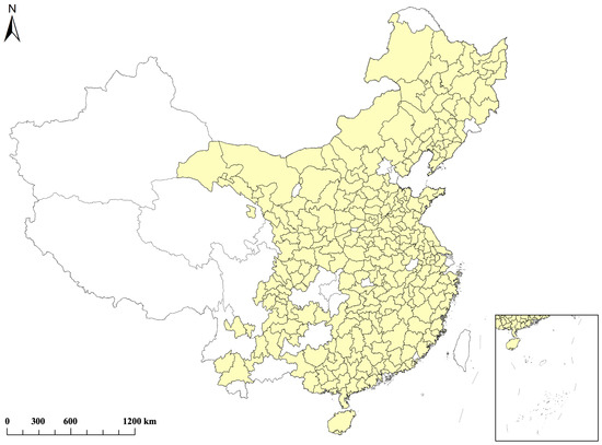
Figure 3.
Location map of the study area.
3.2. Selection of Variables
3.2.1. Explained Variables
The aim of this research was to clarify the impact of the RRUM on the IARH. Given the wide variation in the stock of rural homestead resources across the country, we used data on the area of rural homestead use from 2008 to 2016 to estimate the ‘annual IARH’, which was used as the dependent variable.
3.2.2. Core Explanatory Variable and Threshold Variables
- RRUM: In this paper, we adapted a broad measure of rural–urban mobility to estimate the net rural mobility rate by region from 2009 to 2016, following Ma et al. [49]. In addition, to avoid differences in results arising from different measures of rural population mobility, we also chose the rural population mobility rate (rural household population to rural resident population ratio) as a robustness test to replace the main explanatory variables for the analysis.
- Urban–rural income gap: Scholars have often used the urban–rural income gap as a lens to study the consumption behaviour and lifestyles of rural residents [50]. We therefore used this variable to analyse the role of the income gap between farmers and urban residents in changes in the use of rural homestead. Specifically, this variable was measured as the ratio of per capita disposable income of urban residents to per capita disposable income of rural residents in each region.
- Rural population density: This variable measures the density characteristics of population clustering in different rural areas. We used the ratio of the area of land used for construction in villages to the rural household population to measure the degree of rural settlement in different areas and, ultimately, for the logarithmic processing of these data.
3.2.3. Control Variables
Following the existing literature on the use of rural homesteads, we choose topographic characteristics, net income per rural resident, natural resource endowment and arable land per capita as control variables. In particular, topographic characteristics were assigned a score of 1–5 to different regions according to five natural topographic conditions (basin, plain, hilly, plateau and mountain), from lowest to highest. In addition, the spatial density of energy was chosen as a measure of natural resource endowment, calculated by dividing the total industrial output of the mining and petroleum industry by the area of land in each region, which was eventually taken as the natural logarithm. Descriptive analysis of all variables is given in Table 1.

Table 1.
Descriptive statistics of the variables.
3.3. Empirical Design
Based on the above theoretical analysis, we used the panel threshold model proposed by Hansen [51] to study the relationship between RRUM and IARH. This model was mainly used to study the non-linear relationship between variables, i.e., when one variable reached a specific value, it caused a sudden change in another variable, and the variable that triggered this change is called the threshold variable, and the critical value is called the threshold value. We mainly designed the following models to test the existence of the threshold effect in three ways: (1) the threshold effect of RRUM on the IARH; (2) using the urban–rural income gap as the threshold to analyse the differential impact of RRUM on the IARH; (3) using rural population density as the threshold to analyse the differential impact of RRUM on the IARH.
where denotes the regression coefficient; subscript represents different cities; subscript represents different years; denotes the indicative function in the threshold variable; and is the threshold variable, which in Equation (1) is the RRUM itself. τ is the threshold value; denotes the RRUM; represents the urban–rural income gap; represents the rural population density; and is a set of control variables that affect the use of rural homesteads, mainly including topographic features, net income per rural resident and arable land per capita. When = , the model would be a single threshold model; when τ1 ≠ τ2, it would be a double threshold model. To overcome the potential heterogeneity problem, and are added to control for the less observable urban (area) and time effects; is a random disturbance term.
Model 1 represents a multiple threshold model with RRUM as the threshold. Model 2 represents a single threshold model, with urban–rural income gap as the threshold. Model 3 represents a single threshold model with rural population density as the threshold. Model 4 is a fixed effects model. In addition, when selecting the ordinary panel model regression, to ensure the robustness and accuracy of the model, the Hausman test was first used to determine whether to use a fixed effects model or a random effects model for the analysis. The test results show a p-value of 0.000, representing a rejection of the original hypothesis. Therefore, we used the fixed effects model as the baseline regression for comparative analysis.
3.4. Endogeneity Discussion
In practice, increases or decreases in the size of the rural homestead may also affect the decisions of rural–urban migrations on a variety of behaviours, such as whether to continue living in the village and whether to go to the city for work. Therefore, the model may suffer from reverse causality. To address the potential endogeneity issue, we used the number of village health centres for the corresponding year in each city as an instrumental variable for the RRUM. Hao and He [52] showed that the construction of infrastructure such as village health centres can avoid accelerated rural exodus, and therefore the number of village health centres can be used as a proxy variable for village health care infrastructure to influence the RRUM. At the same time, this variable is not directly related to the IARH in the region, which meets the requirement of exogeneity of the instrumental variable.
4. Empirical Results
4.1. Threshold Effects and Tests of Truthfulness
For the threshold analysis, 300 bootstrap method tests were used in this research. Table 2 reports the results of the threshold tests for the RRUM, the urban–rural income gap and the rural population density, respectively. The test results show that there was a single threshold for the RRUM at the 1% level of significance and a double threshold at the 5% level of significance. Both the urban–rural income gap and the rural population density had a single threshold at the 5% level of significance.
Table 2.
Self-sampling and significance tests for threshold effects.
Further, we tested the thresholds for truthfulness using the LR test. As can be seen from the likelihood ratio function plots (Figure 4 and Figure 5), the LR statistic corresponding to each threshold is below the dashed line threshold. Therefore, all of the above threshold estimates passed the test of truthfulness.
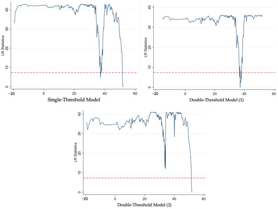
Figure 4.
Estimates of single-threshold and double-threshold for RRUM. Note: The lowest point of the solid line is the corresponding threshold and the red dashed line represents the LR threshold (7.35).
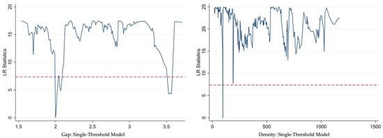
Figure 5.
Estimates of the gap and the density as the threshold variables. Note: The lowest point of the solid line is the corresponding threshold and the red dashed line represents the LR threshold (7.35).
4.2. Regression Results with Different Threshold Variables
We first examined the threshold effect of the RRUM on the IARH in order to analyse the impact of rural–urban migration on the use of rural homesteads, and the results are shown in Table 3. The regression results show that the existence of two thresholds for the RRUM caused a structural change in its relationship with the IARH. At lower values of RRUM (mobility ≤ 37.124), RRUM had a significant positive effect on IARH, with a coefficient of 0.020, while at moderate values of RRUM (37.124 < mobility ≤ 51.960), the coefficient of effect was 0.006, with a decreasing but statistically insignificant effect. And when the RRUM reached a high level (mobility > 51.960), the coefficient of its effect turned from positive to negative (the coefficient is −0.014) and was significant at the 1% statistical level. The above results suggest that there is a marginal decreasing contribution to the IARH with the RRUM when the threshold is not reached. When the threshold is reached, there is a negative effect of the RRUM on the IARH. The results of this analysis validate the our H1.
Table 3.
Estimation results of the model with the RRUM as the threshold variable.
To test the robustness of the results, we used a fixed effects model to analyse the relationship between the quadratic term of the RRUM and IARH (column 3 of Table 3). It can be seen that the squared term of the RRUM was negative at the 1% significance level, further validating the inverted U-shaped relationship between the RRUM and the IARH. In the analysis of the other control variables (column for Panel Model in Table 3), it can be seen that the regional rural–urban income gap significantly suppressed the IARH, with an effect coefficient of −0.295. This suggests that as the rural–urban income gap increases, the migrating populations may no longer return to their hometowns and the demand for new rural homesteads will fall. Rural population density significantly suppressed the IARH, while per capita arable land area significantly increased the IARH. This suggests that sparsely populated conditions are more likely to increase the IARH. In addition, the higher the altitude (terrain), the higher the IARH, indicating that the more uninhabitable the terrain is, the less strict the supervision may be, creating illegal land occupation and the area over the limit, and thus promoting an increase in the area of rural homesteads. The net income per rural resident in the region will contribute to the increase in the IARH, indicating that with the economic development and the increase in farmers’ income, farmers’ demands for rural homesteads have been met to a greater extent, thus promoting “house building consumption” to a certain extent. Furthermore, the better the natural resource endowment of the region, the more the IARH will be suppressed, to a certain extent. This may be due to the fact that some resource-based cities are more prone to irrational land use. In mining towns, for example, the threat of encroachment and ecological damage caused by resource extraction makes it easier to promote the concentration of villages around mining areas, thus curbing the rapid growth of rural homestead.
Further, the regression of the instrumental variable in column 4 of Table 3 reports the results of the second stage of the regression, with the number of village health centres as the instrumental variable. Firstly, we tested the validity of the instrumental variable. The estimation results of the first stage revealed that the number of village health centres had a significant negative effect on the RRUM. In other words, the increase in the number of village health centres can effectively curb the large rural exodus. The F-statistic is 29.412, which satisfies the requirement of F-statistic value > 10, implying that the instrumental variable satisfies the conditions of exogeneity and correlation. The estimation results of the second stage show that the effect of the RRUM on the IARH still exhibited an inverted U-shaped relationship. Hypothesis 1 was therefore further tested.
Next, we tested whether the rural–urban income gap is a threshold variable. As can be seen from the first column of Table 4, the urban–rural income gap in different regions affects the relationship between the RRUM and the rate IARH. Combined with the threshold values in Table 2, it can be seen that when the urban–rural income gap was below 2., an increase in the RRUM raised the IARH. Conversely, when the value of the urban–rural income gap was ≥2, the RRUM showed a significant negative relationship with the IARH; thus Hypothesis 2 was tested. Finally, we tested whether the rural population density was a threshold variable. As can be seen from the second column of Table 4 and the threshold values in Table 2, when the rural population density was below 96.410, an increase in the RRUM significantly raised the IARH. However, when the rural population density was higher than 96.410, there was no significant effect relationship between the two, so Hypothesis 3 was tested.
Table 4.
Results of model estimation with gap or density as threshold variables.
4.3. Robustness Tests
The relationship between the RRUM and the IARH was tested by means of instrumental variables in the previous section. In order to further verify the robustness of the above threshold estimates, we used the following two approaches to test the robustness of the model while maintaining the original model form (Table 5). (1) Substitution of the main explanatory variables. We replaced the RRUM in the model with the ‘rural population mobility rate’ and ran the regression. The results showed that the double threshold effect of the rural population mobility rate on the IARH was still significant. (2) Excluding the city where the pilot areas of the rural homestead system reform are located. Although the time period studied in this research barely includes the new cycle of pilot reforms to China’s homestead system, certain pilot areas may have had some specificity prior to the start of the reforms. We therefore re-ran the threshold regressions after excluding all pilot cities of the rural homestead use system to further check the robustness of the findings. The results showed that the single threshold effect was significant at the 1% statistical level and the double threshold effect was significant at the 5% statistical level. With the exception of the intermediate stage, which was not significant, the RRUM changed from positive to negative at the 1% level of significance, affecting the IARH. The above further validated the robustness of the regression results in this research.
Table 5.
Robustness test results.
5. Heterogeneity and Discussion of Mechanisms
Both natural factors, such as resource endowments and topographical conditions, and social factors, such as institutional and cultural contexts, may influence the relationship between RRUM and IARH to varying degrees, and thus the relationship between the two may vary considerably between regions. We analysed the heterogeneity of the threshold effect in terms of urban-specific factors, such as region and ethnicity, that may influence the use of rural homestead use and the perception of rural house building. All subgroups were tested without changing the form of the model. The threshold model was first tested, and if there was no threshold, a fixed effects panel model was used for comparative analysis. The full results of the heterogeneity analysis are reported in Table 6 and Figure 6.
Table 6.
Analysis of regional heterogeneity based on different classifications.
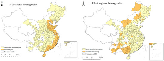
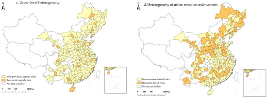
Figure 6.
Regional heterogeneity in the presence of threshold effects.
As can be seen from Figure 6a, the threshold effect of the RRUM on the IARH was only found in the central and western regions (see Note 2). In contrast, in the eastern region, IARH was significantly positively affected as RRUM increased (see the eastern region column in Table 6). The possible explanation is that the value of land, the level of economic development and the living environment are generally higher in the eastern regions than in the central and western regions. Whether from the perspective of building investment or improving the living environment, rural migrants in the eastern region may have more incentive to return to their hometowns after working in the cities and to build homesteads in their hometowns. Many studies have shown that areas where clan values are prevalent and minority nationalities live together have a greater sense of ‘Falling Leaf Returns To Root’. That is, when they get older, rural–urban migrants usually choose to return to their hometowns to retire. Therefore, even though there is a high RRUM, these farmers will choose to build farmhouses within the village or even apply for more rural homesteads for their offspring to divide or for when they get married, thus accelerating the IARH (as shown in Figure 6b). Similarly, a significant positive effect of RRUM on IARH can be seen in the minority nationality column in Table 6.
As can be seen from the provincial capital cities column in Table 6, the RRUM in provincial capitals significantly increased the IARH at a statistical level of 10%. However, the threshold effect between the two was only present in non-provincial capital cities (Figure 6c). That is, rural–urban migrants in developed areas will have a stronger incentive to return to their hometowns, and the RRUM consistently showed a significant positive correlation with the IARH. In the heterogeneity analysis of resource-based cities, the threshold effect of the RRUM was found to be present in most non-resource-based cities (Figure 6d), while there was no significant relationship between the two in resource-based cities (see the resource-based cities column in Table 6). Resource-based cities, facing the threat of the ‘resource curse’, tend to show a higher dependence on land use, especially for construction in rural and suburban areas, thus increasing the potential for encroachment on rural homesteads and the inhibition of the rapid expansion of IARH.
6. Discussion of Spatial Spillover Effects
There was a peer effect and spatial correlation between farmers’ behavioural decisions found in some scholarly studies [53,54,55]. We conducted a preliminary spatial description analysis for RRUM and IARH separately to further discuss the influence relationship between RRUM and IARH (as shown in Figure 7). Figure 7 reflects the spatial distribution of the RRUM and the IARH in China in 2009 and 2016. In terms of time trends, both the RRUM and the IARH showed an increasing trend across most of the country. From a regional perspective, the RRUM was more pronounced in the northeast and southeast coastal regions, while the IARH in the central region was increasing. In terms of spatial clustering characteristics, both the RRUM and the IARH showed similar patterns of change in some regions, so there may be some spatial correlation characteristics. To verify the existence of such an effect, we used a spatial econometric model to test the spatial spillover effect of the RRUM on the IARH. Firstly, a Global Moran’s I index was used to analyse and test the spatial autocorrelation between the RRUM and the IARH, which was an important basis for determining whether the RRUM generated spatial spillover effects. The results are shown in Table 7. During the period 2009–2016, the Moran index for the RRUM was all positive (0.088–0.156) and the Moran index for the IARH was also all positive (0.135–0.225). Except for individual years, both variables passed the 1% significance level test, indicating that there was significant spatial autocorrelation between the RRUM and the IARH. Therefore, we could choose a suitable spatial econometric model to further decompose this spatial spillover effect.
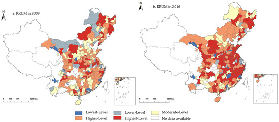
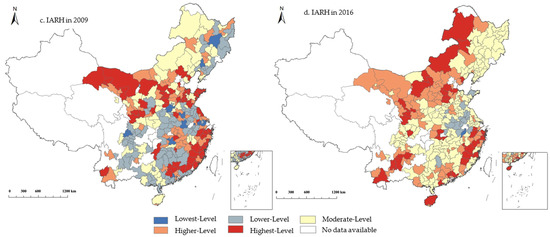
Figure 7.
Spatial distribution of RRUM and IARH in China from 2009 to 2016.
Table 7.
Global Moran’s I index of the RRUM and the IARH.
Next, we selected a spatial Durbin fixed effects model to further investigate the spatial spillover effect using the robust Lagrange multiplier (R LM), the Wald test, the LR test and the Hausman test, in turn. The model form is as follows.
where represents the IARH in year of the th city; includes the RRUM and various control variables; ρ and λ represent the two spatial autocorrelation coefficients; represents the weight matrix of neighbouring spaces; and represent the random error terms. When = 0, = 0 and ≠ 0, the above model can be simplified to an SLM model; when = 0, ≠ 0 and = 0, the model can be simplified to an SEM model.
As can be seen from Table 8, the estimated value of the spatial autoregressive coefficient ρ was 0.095, and it was significant at the 1% statistical level, proving that there is a certain spatial spillover effect of the IARH to the surrounding areas, and Hypothesis 4 is verified. The coefficients of the independent variable and the lagged variable showed that an increase in the RRUM had a positive spatial spillover effect on the IARH, while the indirect effect also confirmed the existence of this spatial spillover effect. In other words, the RRUM not only affected the use of rural homesteads in the region, but also had an indirect spillover effect on the surrounding areas.
Table 8.
Spatial spillover effects of the RRUM on the IARH.
7. Conclusions and Recommendations
This research analysed a particular phenomenon of urbanisation in China, namely, the continuous increase in the area of rural land use, while rural migrants continue to move to the cities. We used data from 2009 to 2016 for each city and used a threshold model to analyse the phased relationship between the RRUM and the IARH, as well as regional variability.
In this study, we found that there is a phased pattern of “dependency” on land in the process of rural–urban migration. Firstly, the threshold model identified an ‘inverted U-shaped’ double threshold effect of the RRUM on the IARH. In other words, the RRUM had an initial growth-boosting effect on the IARH, but this boost was phased in and gradually tailed off as the RRUM increased. Secondly, the relationship between the RRUM and the IARH depends to some extent on rural population density and the regional urban–rural income gap. Specifically, as the regional urban–rural income gap increased, there was an inverted U-shaped threshold effect of the RRUM on the IARH, which increased first and then decreased. As rural population density increased, the contribution of the RRUM to the IARH showed a trend of diminishing marginal benefits. Thirdly, the threshold effect of the RRUM on the IARH was mainly found in the central and western regions, non-minority nationality areas, non-provincial capital cities and non-resource-based cities. Lastly, the RRUM can not only directly affect the local IARH, but also indirectly affect the surrounding areas through spatial spillover effects.
This research has several drawbacks. Firstly, the data used in this study did not include data on the latest round of reforms to the homestead system. This was mainly due to the slow progress of the current reform of the homestead system, which makes it difficult to reflect changes in the macro data at the national level. Moreover, the land use data for the latest years differed from the previous round of land use surveys in terms of land category identification, and therefore it was too difficult to conduct a coherent, long-term panel data study using the latest data. Therefore, the findings of this research apply mainly to non-pilot areas in China prior to the new round of reforms to the rural homestead system. In the future, subject to the availability of data, consideration may be given to comparing whether the reform of the homestead system has led to a discussion of changes in the relationship between rural migrations and land use studied in this research. Secondly, this research used macro-level data to study the behaviour of rural–urban migrants in occupying rural land during migration. However, the reality is that rural–urban migrants vary greatly, and there is a wide gap between the behavioural decisions and ideologies of different individuals. In the future, additional research on the behavioural decisions of individual rural migrants could be considered using questionnaire data.
This research suggests the following policy implications based on its findings.
Firstly, from an urban perspective, a better housing security system for migrant workers should be established to reduce the uncertainty of their housing that leads them to build farmhouses in their hometowns. The reform of the household registration system should be further deepened and the development of “equal rights to rent and purchase” should be promoted. At the same time, the focus should be on the social security role of the rural–urban migrant population, so that migrant workers can enjoy the same public services and social security in the city and change the perception migrants may have that the rural homestead is the only way to protect themselves against risks.
Secondly, from the perspective of rural homestead use, we should fully understand the “inverted U-shaped” development pattern of rural–urban mobility, in which rural migrants rely on rural homesteads. Combined with the urban heterogeneity analysis in this research, the management and institutional reform of rural homestead use should be promoted according to local conditions in accordance with the law of population outflow. For the eastern, coastal, economically developed or densely populated regions, the RRUM in these regions has not reached the top of the “inverted U-shape”. In addition, there is still a strong economic dependence on homesteads in these regions, as farmers move to the cities, and demand for new homesteads is strong. These areas can appropriately develop special rural industries and small town construction, improve the quality of public service provision and narrow the gap between urban and rural areas. By realising the return of some migrant workers to their hometowns for employment and local urbanisation, the problem of some idle farm buildings and wasted rural land resources can be further resolved. For areas with a large rural population outflow and a large number of unused rural homesteads, these areas have reached the right side of the “inverted U-shape”, and should promote the work of consolidating and reclaiming rural homesteads appropriately, revitalising unused natural resources assets, intensively and economically using rural land and establishing a system of the withdrawal of rural homesteads with compensation.
Thirdly, in terms of regional effects, policy makers should consider reducing the phenomenon of unreasonable usage of rural homesteads due to deep-rooted concepts such as social networks and customs and culture in certain regions from a spatial perspective. In particular, in promoting the reform of the rural homestead system, it is important to promote the linkage of management with the change in customs and traditions in the countryside, so as to reduce the phenomenon of “rural house building fever” in rural areas due to marriage contracts. In the countryside, it is important to put an end to the illegal overbuilding of rural homestead due to social status and status symbols.
Author Contributions
R.Y. contributed to the idea, data curation, methodology, formal analysis and the original draft of the manuscript; J.Y. contributed to the project administration, review and editing and funding acquisition; L.S. contributed to the conceptualization, the original draft of the manuscript and review and editing. All authors have read and agreed to the published version of the manuscript.
Funding
This research was supported by the Renmin University of China “Special Funds for Guiding the Development of World-Class Universities (Disciplines) and Special Features of Central Universities”.
Data Availability Statement
Not applicable.
Conflicts of Interest
The authors declare no conflict of interest.
Notes
| 1 | Data are obtained from http://tddc.mnr.gov.cn/to_Login (accessed on 3 July 2023). |
| 2 | Eastern regions include cities in Hebei, Shandong, Jiangsu, Zhejiang, Fujian, Guangdong and Hainan provinces. The rest of the cities are included in the analysis of the central and western regions. The criteria for classifying ethnicity as heterogeneity were whether the region is a Han area or an area inhabited by ethnic minorities. |
References
- Song, Y.J.; Zhang, C.Y. City size and housing purchase intention: Evidence from rural–urban migrants in China. Urban Stud. 2019, 57, 004209801985682. [Google Scholar] [CrossRef]
- Wang, C.; Pang, Z.; Choi, C.G. Township, County Town, Metropolitan Area, or Foreign Cities? Evidence from House Purchases by Rural Households in China. Land 2023, 12, 1038. [Google Scholar] [CrossRef]
- Hu, F. Homeownership and subjective wellbeing in urban China: Does owning a house make you happier? Soc. Indic. Res. 2013, 110, 951–971. [Google Scholar] [CrossRef]
- Roback, J. Wage, rents, and the quality-of-life. J. Political Econ. 1982, 90, 1257–1278. [Google Scholar] [CrossRef]
- Stawarz, N.; Sander, N.; Sulak, H. Internal migration and housing costs—A panel analysis for Germany. Popul. Space Place 2021, 27, e2412. [Google Scholar] [CrossRef]
- Bjerke, L.; Mellander, C. Mover stayer winner loser a study ofincome effects from rural migration. Cities 2022, 130, 103850. [Google Scholar] [CrossRef]
- Ji, Z.; Xu, Y.; Sun, M.; Liu, C.; Lu, L.; Huang, A.; Duan, Y.; Liu, L. Spatiotemporal characteristics and dynamic mechanism of rural settlements based on typical transects: A case study of zhangjiakou city, China. Habitat Int. 2022, 123, 102545. [Google Scholar] [CrossRef]
- Bao, H.J.; Xu, Y.L.; Zhang, W.Y.; Zhang, S. Has the monetary resettlement compensation policy hindered the two-way flow of resources between urban and rural areas? Land Use Policy 2020, 99, 104953. [Google Scholar] [CrossRef]
- Wang, Y.Q.; Wang, Z.H.; Zhou, C.S.; Liu, Y.; Liu, S. On the settlement of the floating population in the Pearl River Delta: Understanding the factors of permanent settlement intention versus housing purchase actions. Sustainability 2020, 12, 9771. [Google Scholar] [CrossRef]
- Yang, Y.; Liu, Y.; Li, Y.; Li, J. Measure of Urban-Rural Transformation in Beijing-Tianjin-Hebei Region in the New Millennium: Population-Land-Industry Perspective. Land Use Policy 2018, 79, 595–608. [Google Scholar] [CrossRef]
- Sehrawat, M.; Giri, A.K. Panel Data Analysis of Financial Development, Economic Growth and Rural-Urban Income Inequality Evidence from SAARC Countries. Int. J. Soc. Econ. 2016, 43, 998–1015. [Google Scholar] [CrossRef]
- Wang, Y.; Liu, Y.; Li, Y.; Li, T. The Spatio-Temporal Patterns of Urban-Rural Development Transformation in China since 1990. Habitat Int. 2016, 53, 178–187. [Google Scholar] [CrossRef]
- Li, H.; Wang, L.J. Housing Price, Price-Income Ratio and Long-Term Residence Intention of the Floating Population: Evidence from the Floating Population in China. Econ. Geogr. 2019, 39, 86–96. [Google Scholar]
- Zhang, Y. Migrant Workers’ Willing of Hukou Register and Policy Choice of China Urbanization. Chin. J. Popul. Sci. 2011, 2, 14–26. [Google Scholar]
- Kelly, D. Reincorporating the Mingong: Dilemmas of citizen status. In Migration and Social Protection in China; World Scientific Publishing Co.: Singapore, 2008; pp. 17–30. [Google Scholar]
- Whyte, M.K.; Whyte, M.K. The paradoxes of rural-urban inequality in contemporary China. In One Country, Two Societies: Rural-Urban Inequality in Contemporary China; Harvard University Press: Cambridge, MA, USA, 2010. [Google Scholar]
- Cheng, W.; Cheng, S.; Wu, H.; Wu, Q. Homesteads, Identity, and Urbanization of Migrant Workers. Land 2023, 12, 666. [Google Scholar] [CrossRef]
- Wu, Y.; Zhou, Y.; Liu, Y. Exploring the outflow of population from poor areas and its main influencing factors. Habitat Int. 2020, 99, 102161. [Google Scholar] [CrossRef]
- Huang, K.; Xia, F. Classification of Rural Relative Poverty Groups and Measurement of the Influence of Land Elements: A Questionnaire-Based Analysis of 23 Poor Counties in China. Land 2023, 12, 918. [Google Scholar] [CrossRef]
- Tang, S.; Hao, P.; Feng, J. Consumer behavior of rural migrant workers in urban China. Cities 2020, 106, 102856. [Google Scholar] [CrossRef]
- Zang, Y.; Yang, Y.; Liu, Y. Understanding rural system with a social-ecological framework: Evaluating sustainability of rural evolution in Jiangsu province, South China. J. Rural. Stud. 2021, 86, 171–180. [Google Scholar] [CrossRef]
- He, Y.; Xie, H.; Peng, C. Analyzing the behavioural mechanism of farmland abandonment in the hilly mountainous areas in China from the perspective of farming household diversity. Land Use Policy 2020, 99, 104826. [Google Scholar] [CrossRef]
- Meng, L. Permanent migration desire of Chinese rural residents: Evidence from field surveys, 2006–2015. China Econ. Rev. 2020, 61, 101262. [Google Scholar] [CrossRef]
- Zhang, T.; Zhu, Y.; Li, L.Y. The residential location choices of returned migrant workers in the context of local urbanization——A case study of Yongcheng city in Henan Province. Econ. Geogr. 2017, 37, 84–91. (In Chinese) [Google Scholar]
- Tan, R.; Wang, R.; Heerink, N. Liberalizing rural-to-urban construction land transfers in China: Distribution effects. China Econ. Rev. 2020, 60, 101147. [Google Scholar] [CrossRef]
- Niu, X.; Liao, F.; Liu, Z.; Wu, G. Spatial–Temporal Characteristics and Driving Mechanisms of Land–Use Transition from the Perspective of Urban–Rural Transformation Development: A Case Study of the Yangtze River Delta. Land 2022, 11, 631. [Google Scholar] [CrossRef]
- McKenzie, D.; Rapoport, H. Self-selection patterns in Mexico-U.S. migration: The role of migration networks. Rev. Econ. Stat. 2010, 92, 811–821. [Google Scholar] [CrossRef]
- Tang, S.; Hao, P.; Huang, X. Land conversion and urban settlement intentions of the rural population in China: A case study of suburban Nanjing. Habitat Int. 2016, 51, 149–158. [Google Scholar] [CrossRef]
- Harris, J.; Todaro, M. Migration, unemployment and development: A two-sector analysis. Am. Econ. Rev. 1970, 60, 126–142. [Google Scholar]
- Zou, J.; Chen, Y.; Chen, J. The complex relationship between neighbourhood types and migrants’ socio-economic integration: The case of urban China. J. Hous. Built Environ. 2020, 35, 65–92. [Google Scholar] [CrossRef]
- Zhang, G.C.; Zhang, S.H.; Gu, H.Y. Farmers’ Income, Land Security and Farmland Withdrawal -Empirical Analysis Based on Micro Survey Data in the Yangtze River Delta. Economist 2020, 9, 104–116. [Google Scholar]
- Rao, J. Comprehensive land consolidation as a development policy for rural vitalisation: Rural In Situ Urbanisation through semi socio-economic restructuring in Huai Town. J. Rural Stud. 2022, 93, 386–397. [Google Scholar] [CrossRef]
- Wu, Y.; Zha, Y.; Ge, M.; Sun, H.; Gui, H. The Impact of Urban Health Care on Migrants’ Settlement Intention: Evidence from China. Sustainability 2022, 14, 15085. [Google Scholar] [CrossRef]
- Zou, J.; Chen, J.; Chen, Y. Hometown landholdings and rural migrants’ integration intention: The case of urban China. Land Use Policy 2022, 121, 106307. [Google Scholar] [CrossRef]
- Peng, J.C.; Wu, Q.; Qian, C. Measuring Contribution of Rural Land Value Increment to Famers’ Urbanization. Popul. J. 2017, 6, 51–61. [Google Scholar]
- Li, Y.H.; Liu, N.N.; Li, X.Q. Farmland Circulation, Housing Choice and Peasant-Workers’ Citizenization. Econ. Geogr. 2019, 11, 165–174. [Google Scholar]
- Yang, J.H.; Zhang, J.J.; Wu, M. My Home Is Where My Heart Is: Regional Disparity and Self-identity of Migrants in China. Popul. Econ. 2016, 4, 21–33. [Google Scholar]
- Zhao, Q.L.; Jiang, G.H.; Ma, W.Q.; Zhou, D.Y.; Qu, Y.B.; Yang, Y.T. Social security or profitability? Understanding multifunction of rural housing land from farmers’ needs: Spatial differentiation and formation mechanism—Based on a survey of 613 typical farmers in Pinggu District. Land Use Policy 2019, 86, 91–103. [Google Scholar]
- Gan, W.Y. An Empirical Study of the Identity, Emotional Commitment and Turnover Intention of the New Generation Migrant Workers from the Rural Areas in the Perspective of the Organizational Support. J. Manag. 2018, 31, 36–49. [Google Scholar]
- Zhang, M.; Zhu, C.J.; Nyland, C. The Institution of Hukou-based Social Exclusion: A Unique Institution Reshaping the Characteristics of Contemporary Urban China. Int. J. Urban Reg. Res. 2014, 38, 1437–1457. [Google Scholar] [CrossRef]
- Zhong, S.; Wang, M.; Zhu, Y.; Chen, Z.; Huang, X. Urban expansion and the urban–rural income gap: Empirical evidence from China. Cities 2022, 129, 103831. [Google Scholar] [CrossRef]
- Du, Y.; Zhao, Z.; Liu, S.; Li, Z. The Impact of Agricultural Labor Migration on the Urban–Rural Dual Economic Structure: The Case of Liaoning Province, China. Land 2023, 12, 622. [Google Scholar] [CrossRef]
- Smailes, P.; Argent, N.; Griffin, T. Rural population density: Its impact on social and demographic aspects of rural communities. J. Rural Stud. 2022, 18, 385–404. [Google Scholar] [CrossRef]
- Bi, G.; Yang, Q. The spatial production of rural settlements as rural homestays in the context of rural revitalization: Evidence from a rural tourism experiment in a Chinese village. Land Use Policy 2023, 128, 106600. [Google Scholar] [CrossRef]
- Liu, Y.S.; Zou, L.L.; Wang, Y.S. Spatial-temporal characteristics and influencing factors of agricultural eco-efficiency in China in recent 40 years. Land Use Policy 2020, 97, 104794. [Google Scholar] [CrossRef]
- Li, T.; Feng, C.; Xi, H.; Guo, Y. Peer Effects in Housing Size in Rural China. Land 2022, 11, 172. [Google Scholar] [CrossRef]
- Ioannides, Y.M.; Loury, L.D. Job information networks, neighborhood effects, and inequality. J. Econ. Lit. 2004, 42, 1056–1093. [Google Scholar] [CrossRef]
- Hung, L.-W.; Peng, S.-K. Rural-Urban Migration with Remittances and Welfare Analysis. Reg. Sci. Urban Econ. 2021, 91, 103629. [Google Scholar] [CrossRef]
- Ma, L.; Liu, S.; Tao, T.; Gong, M.; Bai, J. Spatial reconstruction of rural settlements based on livability and population flow. Habitat Int. 2022, 126, 102614. [Google Scholar] [CrossRef]
- Chanieabate, M.; He, H.; Guo, C.; Abrahamgeremew, B.; Huang, Y. Examining the Relationship between Transportation Infrastructure, Urbanization Level and Rural-Urban Income Gap in China. Sustainability 2023, 15, 8410. [Google Scholar] [CrossRef]
- Hansen, B.E. Threshold Effects in Non-dynamic Panels: Estimation, Testing, and Inference. J. Econom. 1999, 93, 345–368. [Google Scholar] [CrossRef]
- Hao, P.; He, S.J. What is holding farmers back? Endowments and mobility choice of rural citizens in China. J. Rural Stud. 2022, 89, 66–72. [Google Scholar] [CrossRef]
- Chen, Z.; Liu, X.; Lu, Z.; Li, Y. The expansion mechanism of rural residential land and implications for sustainable regional development: Evidence from the Baota district in China’s Loess Plateau. Land 2021, 10, 172. [Google Scholar] [CrossRef]
- Sargeson, S. Subduing “the rural house-building craze”: Attitudes towards housing construction and land use controls in four Zhejiang villages. China Q. 2002, 172, 927–955. [Google Scholar] [CrossRef]
- Iannaccone, L.R. Sacrifice and stigma: Reducing free-riding in cults, communes, and other collectives. J. Political Econ. 1992, 100, 271–291. [Google Scholar] [CrossRef]


Disclaimer/Publisher’s Note: The statements, opinions and data contained in all publications are solely those of the individual author(s) and contributor(s) and not of MDPI and/or the editor(s). MDPI and/or the editor(s) disclaim responsibility for any injury to people or property resulting from any ideas, methods, instructions or products referred to in the content. |
© 2023 by the authors. Licensee MDPI, Basel, Switzerland. This article is an open access article distributed under the terms and conditions of the Creative Commons Attribution (CC BY) license (https://creativecommons.org/licenses/by/4.0/).