Article

Balancing Urban Expansion and Ecological Connectivity through Ecological Network Optimization—A Case Study of ChangSha County

1
School of Architecture and Art, Central South University, Changsha 410083, China
2
Research Center of Human Settlements, Central South University, Changsha 410083, China
3
School of Architecture, South China University of Technology, Guangzhou 510641, China
4
School of Architecture and Planning, Hunan University, Changsha 410082, China
*
Authors to whom correspondence should be addressed.
Land 2023, 12(7), 1379; https://doi.org/10.3390/land12071379
Submission received: 13 June 2023 / Revised: 5 July 2023 / Accepted: 7 July 2023 / Published: 11 July 2023

Abstract

:
The counties have experienced urban expansion and landscape pattern fragmentation. As carriers of new urbanization, the balanced development between urban expansion and landscape connectivity in the counties needs to be emphasized. The uncontrolled expansion of land should be discouraged and planners need to clarify land use expansion patterns. Using Changsha County as the study area, the characteristics of the landscape pattern between 2000 and 2020 were analyzed. The morphological spatial pattern analysis and landscape connectivity method (CMSPACI), as well as the minimum cumulative resistance (MCR) model, was used to construct the ecological network. We also explored the most appropriate corridor width using the buffer zone to guide future land use planning and ecological network planning. The results show that based on CMSPACI the total area of ecological sources identified was 304.91 km2, encompassing a large area of forest parks. The total length of the 25 ecological corridors identified by the MCR model was 431.97 km. Ecological sources and corridors are missing in the central region; so, their pattern was optimized using landscape connectivity and the absence of location as selection criteria. The optimized network indices showed significant improvement. The width of the ecological corridors should be controlled in order to be in the range of 30 m to 50 m to maximize the effect of the corridors on species dispersal and migration. Our proposed research framework for the construction and optimization of EN in Changsha County can provide ideas to balance the contradictions between urban expansion and landscape connectivity in Changsha County.

1. Introduction

To alleviate the burden of urban development, the counties have been utilized as significant carriers for a new type of urbanization [1]. However, this has resulted in a significant expansion of the counties and negatively impacted the landscape pattern [2,3,4]. The landscape connectivity of the counties has been reduced, seriously affecting ecological processes such as material and energy flows [2]. Given the importance of sustainable development for the counties, it is necessary to restrain the land changes brought about by uncontrolled urban expansion and to achieve a balanced development of ecological urbanization.
Building an ecological network (EN) can enhance the landscape connectivity of the region, protect the stability of ecosystem functions, and promote biodiversity [5,6]. Currently, ecological network research has been applied in many fields. Examples include conservation and restoration of ecological security patterns [7,8], promoting biodiversity [9], green infrastructure planning [10,11], ecological risk assessment [12,13], ecological space and land use planning [14,15], and restoration of ecosystem services [16]. To achieve the balanced development of a county’s urban expansion and landscape connectivity, ecological protection and land use guidance are necessary. Constructing an appropriate EN is considered an important way to achieve a balanced development of urban expansion and landscape connectivity. However, the current studies of ecological networks have mainly focused on overall conservation measures, and spatial patterns of specific elements and land use guidelines have been neglected [17]. Therefore, the method of the construction should be optimized when conducting county ecological networks.
Based on landscape ecology theory, EN configures landscape elements into a coherent system consisting of ecological sources and ecological corridors [18]. Specifically, EN is formed by connecting ecological sources through corridors, thus strengthening the connections between fragmented patches and enabling species habitat and migration [19]. As an alternative to biological habitats, ecological sources are patches of high ecological value in the landscape; so, their connectivity is important for the efficiency of the entire network. Some scholars directly identified nature reserves [20], urban green area spaces [21], and forest parks [22] with better ecological functions as ecological sources. However, such definitions ignored the landscape connectivity of the patches [23]. The morphological spatial pattern analysis and landscape connectivity method (CMSPACI) classifies patch types and structures based on raster data and calculates the connectivity of each patch [24]. The CMSPACI method is currently used by many scholars to conduct extension studies and is widely applied in the fields of ecological networks, ecological security patterns, and green infrastructure [25].
To connect ecological resources organically and maximize ecological connectivity, many methods have been proposed for the creation of corridors between sources, such as circuit theory [26] and the minimum cumulative resistance (MCR) model [27]. The circuit theory is computed based on the dispersal properties of species. In contrast, the MCR model is based on the “source-sink” theory, which takes into account the connection between horizontal landscape units and has obvious advantages in constructing EN [28]. However, the ecological corridors extracted by the MCR model have directional but not spatial scope, leading to a serious disconnect between EN planning and territorial spatial planning [29]. Some scholars addressed this issue by delineating ecological security pattern zones, but these approaches focused more on delineating protected areas and constructing general conservation patterns [30]. The counties’ land expansion is inevitable in the context of urbanization [31], and land expansion is a major threat to ecological conservation [32]. Under the concept of sustainable development, it is therefore important to emphasize both the importance of urban expansion resulting from economic development and the landscape conservation. This means that it is insufficient to provide conservation strategies for the existing landscape pattern. It is important to provide guidance on future land use and to clarify the form of land change within the scope [33]. Therefore, the land use characteristics at different corridor widths need to be determined. The optimization of EN can be achieved by defining corridor width. Such an EN is more conducive to balancing the contradiction between urban expansion and ecological connectivity.
As the county seat of Changsha City, Hunan Province, Changsha County is ranked among the top 100 counties in China, ranking 10th in the country as a whole and 1st in midwestern China. It bears the burden of balancing economic and ecological development. Therefore, with Changsha County as the study subject, we used the CMSPACI and MCR models to construct and optimize EN and further explore the width of ecological corridors. The objectives of this study were: (1) to analyze the changes in the landscape pattern of Changsha County from 2000 to 2020; (2) to improve the identification of ecological sources through CMSPACI; (3) to assign the coefficient of resistance factors by the spatial principal component analysis (SPCA) method; (4) to simulate and classify ecological corridors based on the MCR model and gravity model; (5) to evaluate the optimized network by the network analysis method; and (6) to explore the ecological corridor widths. This study can provide ideas on how to balance urban expansion and ecological protection in county areas.

2. Materials and Methods

2.1. Study Area

Changsha County covers an area of 175.6 km2 and is located in the eastern part of Hunan Province (112°56′ E–113°36′ E and 27°54′ N–28°38′ N) (see Figure 1). The topography of Changsha County is high in the north and low in the central and southern regions. According to the Köppen classification, the climate in Changsha County is Dfa, with hot summers and cold winters. There are also many rivers in the region with abundant flowing water. As a major transport hub in Hunan Province, Changsha County’s transportation development over the past decade has solidified the foundation for the opening up of the county. In 2020, the total industrial output of Changsha County reached CNY 77.848 billion [26]. It has about one-third of Changsha City’s construction plants, and the industrial level is the highest among all counties in Changsha City [34]. However, there is also the fact that the ecological environment in Changsha County is deteriorating. From 2003 to 2018, 26.94% of the area of Changsha City was severely degraded in terms of ecological environment quality, with Changsha County accounting for the largest share [34].

2.2. Data Sources

The following data were used to conduct this study. The land cover data of Changsha County in 2000, 2010, and 2020 were derived from GlobeLand30 (http://www.globallandcover.com/, accessed on 10 May 2022), with a resolution of 30 m × 30 m and a kappa coefficient of 0.82. Using Arc GIS 10.8, the data were classified as cultivated land, forestland, grassland, wetland, waters, and construction land. Digital elevation data and Landsat8 OLI remote sensing images of 2020 with a resolution of 30 m × 30 m were provided by Geospatial Data Cloud (https://www.gscloud.cn/, accessed on 14 June 2022). The Landsat8 OLI remote sensing imagery was calibrated for radiance and banded in ENVI5.3 to obtain NDBI data. The administrative vector boundary of Changsha County was selected from the national geographical information catalog service, including the administrative boundaries of each town (https://www.webmap.cn/, accessed on 21 June 2022). Road network data for Changsha County were obtained from the Open Street Map website (https://www.openstree tmap.org/, accessed on 5 May 2022). The national roads, provincial roads, urban main roads, secondary roads, and branch roads of Changsha County were obtained by cutting the boundary vector data of Changsha County in Arc GIS10.8.

2.3. Methods

2.3.1. Assessment of Changes in Landscape Pattern

We assessed the spatial variation resulting from urban expansion by quantifying the relative changes in landscape patterns across the years [13]. We selected several indices (including class level and landscape level) related to fragmentation, dominance, and diversity for spatial analysis from previous studies. The indices we chose include total class area (CA), number of patches (NP), edge density (ED), patch density (PD), large patch index (LPI), contagion index (CONTAG), splitting index (SPLIT), Shannon’s diversity index (SHDI), and Shannon’s evenness index (SHEI) [35,36]. The analysis of landscape pattern indices using Fragstats 4.2.1 is currently one of the most important methods for the quantitative analysis of landscape pattern change [37]. Based on the land cover raster maps, we obtained the results of the landscape indices in Fragstats 4.2.1 for 2000, 2010, and 2020 to analyze the landscape pattern changes in Changsha County.

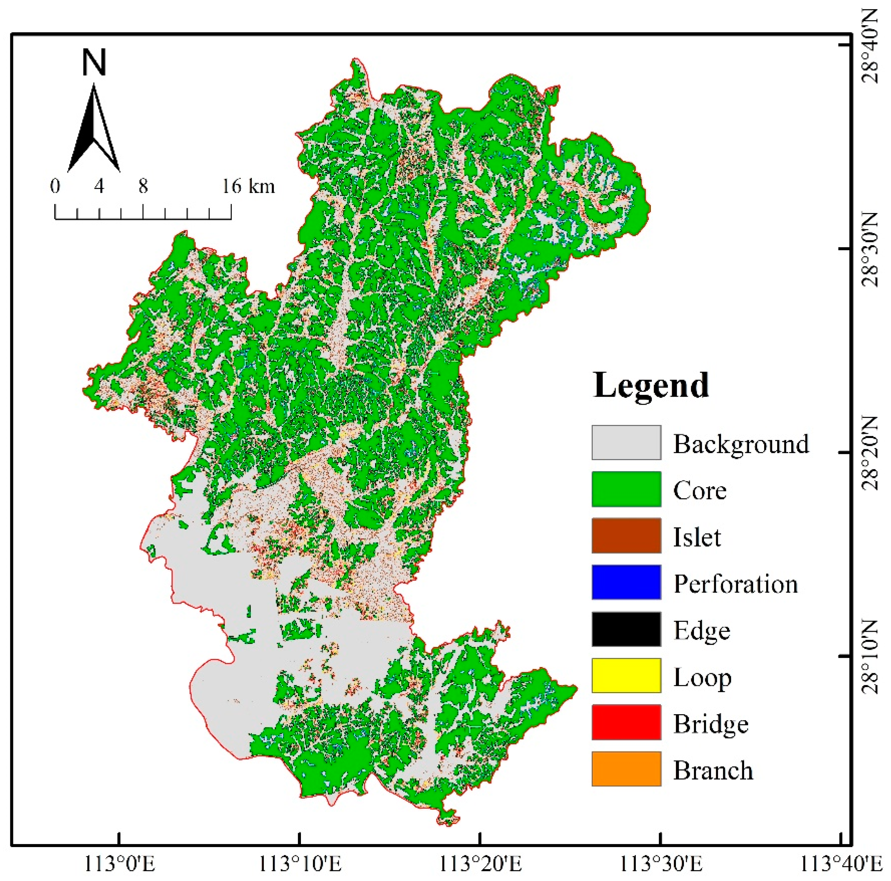
2.3.2. Identification of Ecological Sources Based on CMSPACI

Morphological spatial pattern analysis (MSPA) is an image classification method based on mathematical morphological principles. Through a series of geometric operations such as erosion, dilation, and anchor skeletonization, MSPA can be used to identify patches that play an important role in connectivity. It can divide the binarized raster image into seven non-interfering landscape types (including core, islet, perforation, edge, bridge, loop, and branch) (see Figure 2), and the core area will serve as a candidate for ecological sources [38]. Considering the species requirements for biological habitats [6], in this study forestland, grassland, and wetland were set as prospect data (assign 1) and other land cover types as background data (assign 0). GuidosToolbox 2.8 was used to analyze the morphological spatial pattern of the image. The edge width was set at 30 m to better preserve the landscape information [39]. Core patches larger than 10 km2 were then imported into Conefor 2.6 for connectivity analysis.
The landscape connectivity index represents the value of the landscape patches for species migration and is of great significance for biodiversity protection and ecosystem stability [40]. Numerous indices, such as the possible connectivity index (PC), the integral connectivity index (IIC), and the equivalent connectivity (EC), are now widely adopted in the calculation of landscape connectivity [41]. The PC not only indicates the connectivity of the landscape but can also be used to calculate the patch importance index (dPC). In this paper, we focused on the connectivity of patches and therefore selected PC (Equation (1)) and dPC (Equation (2)) to screen the ecological sources of the study area [42].
P C = i = 1 n j = 1 n a i a j p i j * A L 2
where n is the number of patches, a i and a j denote the area of patches i and j, p i j * is the probability of species dispersal between patches i and j, and A L 2 represents the total area of the landscape within the study area. Note that the PC ranges from [0, 1].
d P C k = P C P C r e m o v e , k P C × 100 %
where P C r e m o v e , k is the connectivity probability index after removing patch k; the higher the value of dPC, the greater the importance of the patch in the landscape.
The distance threshold was set to 1000 m, and the connectivity probability was set to 0.5 [5]. In addition, we further selected core patches with dPC > 2 as ecological sources.

2.3.3. Construction of Ecological Resistance Surface

Natural and artificial factors that are too extreme can have a hindering effect on the migration of species [43]. Based on this, we divided the factors potentially affecting the species into three categories: landscape type, natural conditions, and human disturbance [44]. The land cover indicates the landscape type. Elevation, slope, and vegetation cover (FVC) were selected to represent the resistance factors of natural conditions. Roads and buildings are typical areas of human activity. NDBI can reflect building density, which can further reflect the degree of human aggregation [45]. Transport network density and accessibility have been shown to be positively correlated with population density [46]. So, we used road network density and the normalized difference built-up index (NDBI) to represent the resistance factors of human disturbance. The estimation of road network density was implemented based on the kernel density estimation tool in Arc GIS 10.8, with the bandwidth assigned to 3500 m. Each resistance factor was classified into five levels according to the natural interruption point grading method in Arc GIS 10.8: from 1 to 5, representing the ecological resistance to be overcome by the organism from low to high (see Table 1 and Figure 3).
The SPCA method was used to determine the weights of the factors in this study. It can eliminate the information redundancy caused by the possible correlation between the factors and can comprehensively analyze the spatial characteristics of the data [47]. In this paper, SPCA was performed in Arc GIS 10.8 on the raster data of each resistance factor, and the cumulative contribution rate of each principal component and a table of each principal component feature vector could be obtained (see Table A1 and Table A2 in Appendix A). The principal component loading matrix was further calculated; then, the weight of each factor was expressed by the variance contribution rate of each principal component (see Table 2). The ecological resistance surface was obtained by the weighted sum of the factors as the cost data for the MCR model.

2.3.4. Identification and Classification of Ecological Corridors

The MCR model was used to extract the most favorable pathways between habitat patches for species migration, which are referred to as ecological corridors. It is mathematically expressed as [48]:
M C R = f     m i n j = n i = m ( D i j     R i )
where f is a function reflecting the proportional relationship between the MCR and ( D i j R i ) ; D i j is the distance that the target cell diffuses to from source j to unit i; R i is the ecological resistance of spatial unit i to energy diffusion.
Based on ecological sources and resistance surfaces, the minimum cumulative paths in the study area were generated using the cost distance and cost path modules in Arc GIS 10.8. The gravity model was able to construct an interaction matrix between the sources to indicate the importance of ecological corridors. In this paper, ecological corridors with G i j greater than 0.1 were considered to be important corridors; then, an ecological safety optimization scheme model was proposed. The specific equation is as follows [49]:
G i j = N i N j D i j 2 = 1 p i ln S i 1 p j ln S j L i j / L m a x = L m a x 2 ln S i ln S j L i j 2 p i p j
where G i j is the interaction strength between ecological sources i and j; N i and N j are the weights of ecological sources i and j; D i j is the normalized resistance of the ecological corridor between ecological sources i and j; p i and p j are the resistances of ecological sources i and j; S i and S j are the areas of ecological sources i and j; L i j is the cumulative resistance of the ecological corridor between ecological sources i and j; L m a x is the largest of the cumulative resistances of the ecological corridors between all the ecological source patches.

2.3.5. Optimization of Network

Ecological nodes are generally located in areas that play an important role in the ecological processes of the landscape. They are the most vulnerable parts of ecological functions in ecological corridors. Protecting ecological nodes is crucial to enhancing the stability and connectivity of EN. In previous studies, ecological nodes were located at the intersection of the minimum patch and the maximum patch or in the collection of the minimum paths [50]. In this paper, we extracted the intersection of the least-cost paths as ecological nodes that can provide multiple paths for species migration. Buffers of 15, 30, 50, 100, 150, 200, 300, 400, and 600 m of the current corridor were set in Arc GIS 10.8 to analyze the area of each land cover type occupied by the corridor at different widths.

2.3.6. Assessment of Ecological Network Structure

The network analysis approach is designed to study a network of internal structural properties and functions in combination with graph theoretical approaches. It has been widely used to evaluate the connectivity and integrity of the network. Network closure (α) indicates the number of connected node cycles. The higher the value of the network closure (α), the greater the smoothness. The line point rate (β) characterizes the average number of nodes in the network and is used to represent the complexity of the connected system. The network forms a single loop when β = 1. Network connectivity (γ) is the ratio of the average number of connections between nodes to the maximum possible number of connections in the network and reflects the degree of connectivity of the nodes. Cost ratio (c) describes the connectivity of the EN; the smaller the value, the smaller the cost of building the EN. The calculation formula is defined as follows [51]:
α = l v + 1 2 v 5
β = L V
γ = L 3 ( V 2 )
C = 1 L D
where L is the number of corridors, V is the number of ecological sources, and D denotes the sum of the length of the ecological corridors.

3. Results

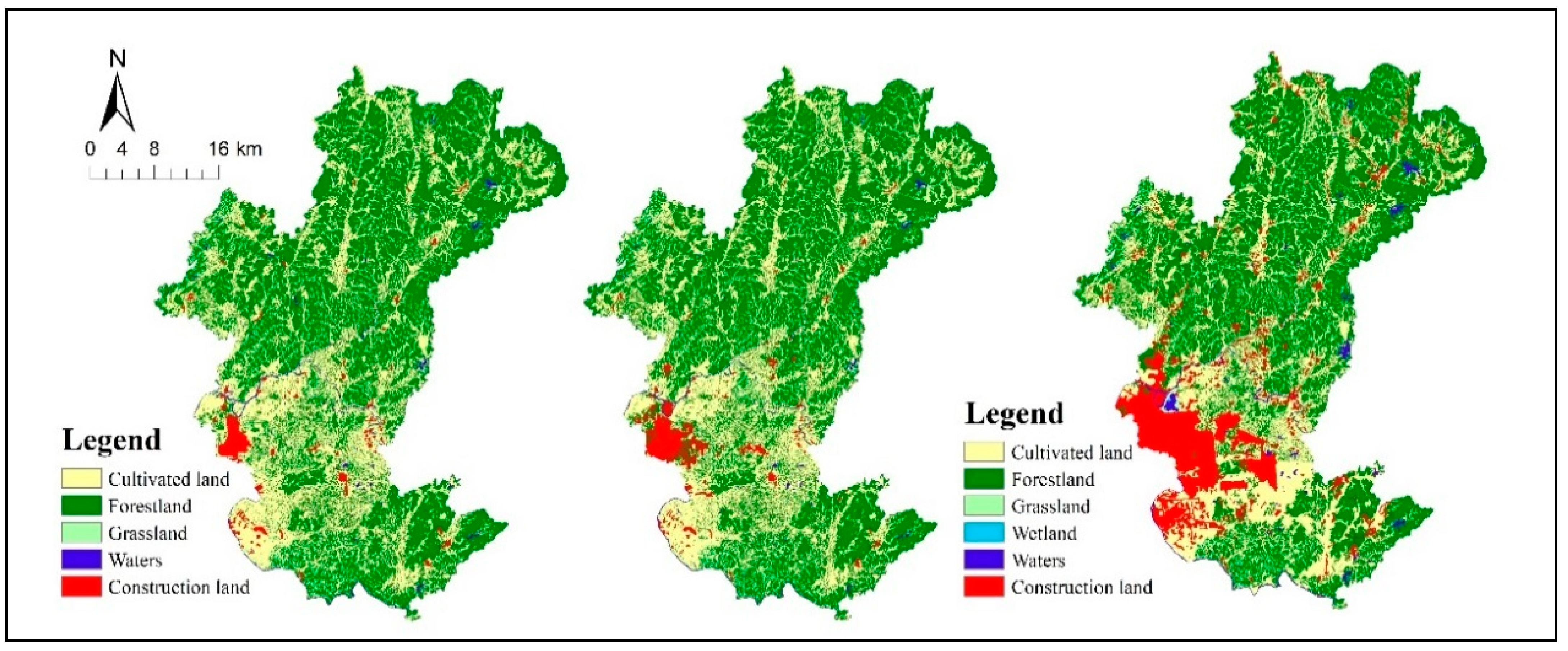
3.1. Landscape Pattern and Land Cover Characteristics

The CA, NP, and PD of the construction land continued to increase, while those for the cultivated land, forestland, and grassland showed a decreasing trend over the 20 years (see Table 3). Compared with other landscape patches, the LPI of the forestland was always at the highest, indicating the highest concentration of forest patches and landscape dominance among all the patch types. However, the LPI of the construction land increased, while the LPI of the cultivated land and forestland showed a slight decrease. The above shows that urban expansion in the central region has clearly led to an increase in the size and density of construction land patches. This has led to the reinforcement of the dominant patch status of the construction land, thus causing the fragmentation of other land types. The ED of the cultivated land, forestland, and grassland decreased continuously from 2000 to 2020. However, the ED value remained high in 2020, with the largest ED for the forestland (value of 88.0292). This indicates that the edges of these landscape patches are long and irregular.
As shown in Table 4, the CONTAG fluctuates slightly, with a decreasing trend from 2000 to 2010 and a continuous increase from 2010 to 2020. The SHDI and SHEI grew at a rate of 1.7% from 2000 to 2010, while the growth rate reached 5.7% and 17.7% from 2000 to 2010. This indicates an increase in landscape heterogeneity during the latter decade. However, the SPLIT showed a continuous rise, indicating that landscape diversification was accompanied by a certain degree of landscape fragmentation.
Figure 4 shows the changes in land cover over 20 years. Over the past two decades, the construction land in central Changsha County has continued to expand eastward and has tended to spread in all directions. In addition, the number of township settlements increased substantially. This indicates a continuous expansion of construction land over a 20-year period. The emergence of wetlands in 2020 contributed to the increase in SHDI and SHEI. However, the values of SHDI and SHEI were still small in 2020. So, in the future, urban planners should create more wetlands and increase the protection of forestland, grassland, and waters.

3.2. Current Ecological Network Pattern

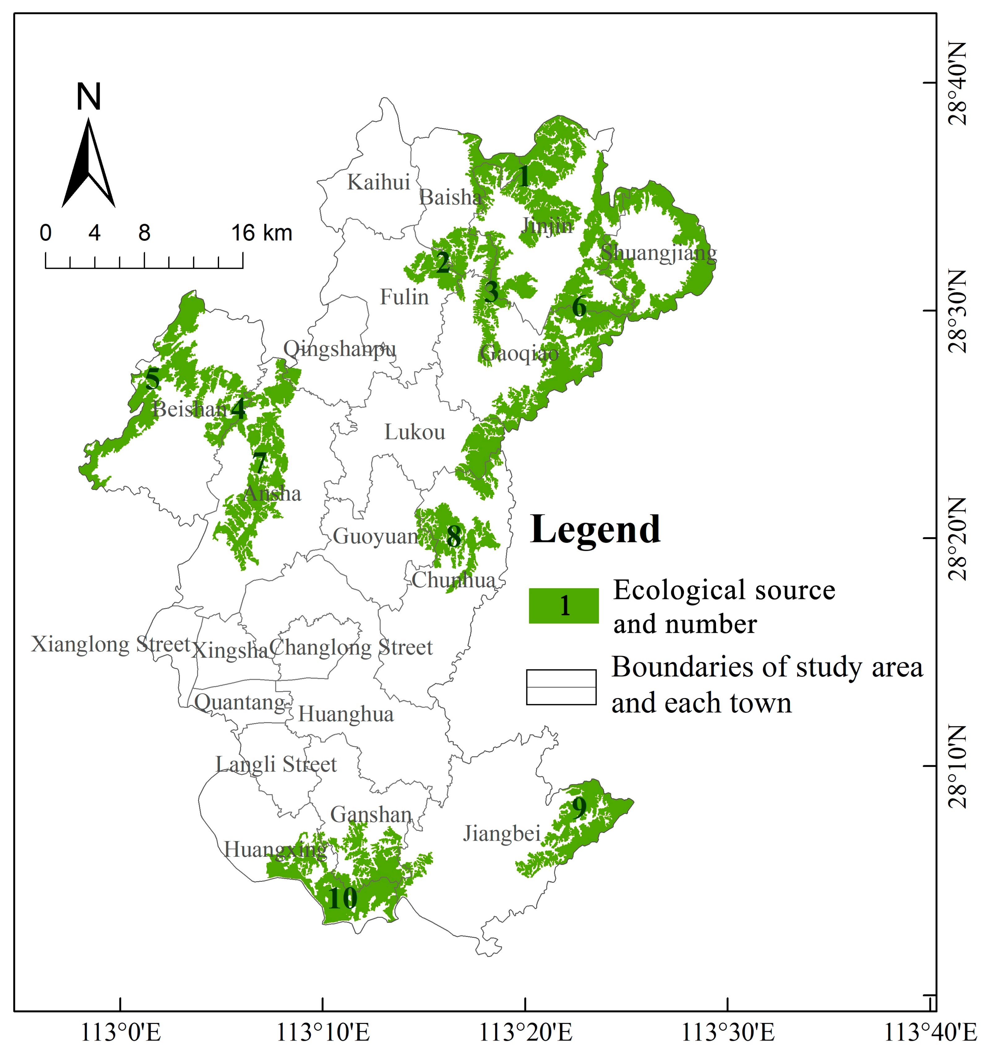
3.2.1. Ecological Sources Pattern

The core is a large patch with ecological value. As can be seen from Table 5, the core accounts for the largest proportion of the foreground data area (69.33%), followed by edges (17.13%), branches (4.00%), islets (3.01%), bridges (2.70%), loops (2.07%), and perforations (1.75%). Moreover, 99.76% of the 71,866 prospective patches were less than 0.5 km2 in area, but their total area was only 37.28%. This reveals the fragmentation of the ecological landscape in the study area.
There were 10 core patches identified as ecological sources based on the CMSPACI results, with a total area of 304.91 km2 (see Table 6). As shown in Figure 5, the ecological sources were unevenly distributed and were basically at the boundary of the study area. The ecological sources were concentrated in the northeast, with a limited distribution in the central and southern regions, especially in the central region. In terms of location, these ecological sources encompassed many important forest parks in Changsha County. Ecological source 5 was located in Beishan Forest Park in Beishan Town; the southern part of ecological source 6 was located in Dashanchong Park in Junction Town; and ecological source 2 was located in Yingzhu Mountain Forest Park in Fulin Town. In addition, the area of ecological sources also varied significantly from town to town, with the largest area being Jinjing town (59.68 km2) and the smallest being Qingshanpu town (1.28 km2).

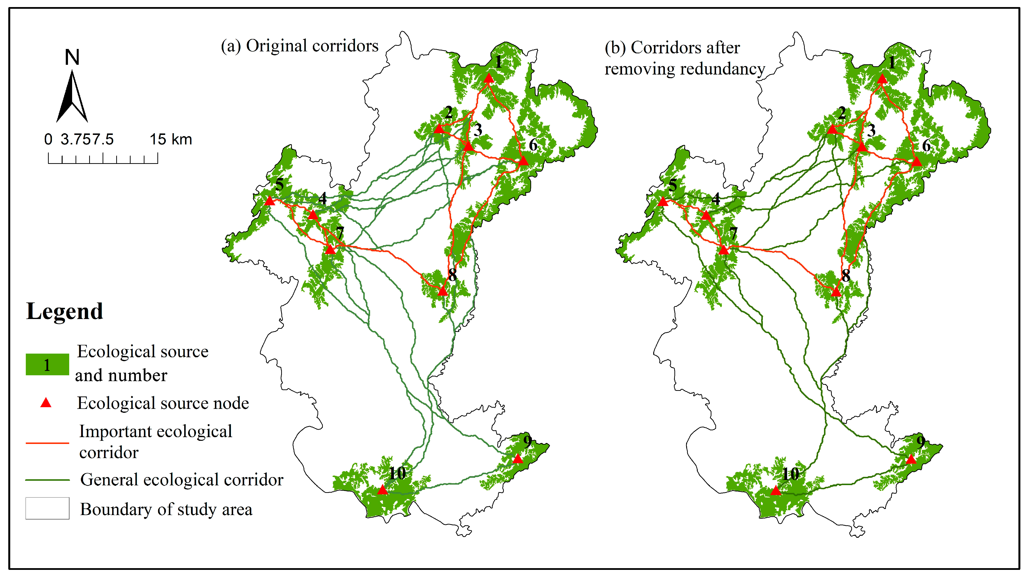
3.2.2. Extraction of Ecological Corridors

Figure 6 shows the distribution of the ecological resistance levels. The resistance was highest in the central west and gradually decreased in the southern and northern directions. The central region bridged the traffic arteries of Changsha City, resulting in higher ecological resistance. However, the resistance gradually decreased closer to the southern and northern borders of the region. As human interference gradually decreased, the land type became predominantly forested. However, Table 7 shows that the high-resistance area accounted for the smallest percentage (8%), and the proportion of mid-low and low resistance was more than half, providing conditions for the creation of stable ecological corridors.
Network 7a, with 45 minimum cost paths of a total length of 1091.13 km, were identified based on resistance (see Figure 7a). We removed the redundant corridors derived from the Arc GIS 10.8 calculations and finally obtained network 7b in the study area (see Figure 7b). It has 25 ecological corridors with a total length of 431.97 km. The corridors were mainly concentrated in the north, with fewer in the center and south. The northern corridors were shorter, while the corridors through the center were longer. Corridors 1–2, 2–5, 5–10, 1–6, 6–8, and 8–9 formed the outer loop of the overall network, while the other corridors branched outward, mainly with source 7 as the center. This combination of an internal tree structure and an external simple ring structure can balance the energy flow in the network with maximum efficiency [52].
We calculated the interaction forces between the ecological sources using the gravity model and found significant differences in the values of the interaction forces (see Table 8). It was determined that there were 11 important corridors with a total length of 168.48 km, and the remaining 14 were general corridors with a total length of 263.49 km. As shown in Figure 7, the important corridors were concentrated among the ecological sources in the northeast, with a lateral link connecting the ecological sources in the east and west. These corridors are important connecting paths with strong interactions between the sources, and therefore, they should be considered for priority protection and construction.

3.3. Network Structure Optimization

3.3.1. Supplementary Ecological Sources and Corridors

It appears that the central western area has a serious network deficiency in the current spatial structure of the EN (see Figure 7b). This means that it is difficult for this region to establish communication with other regions in terms of energy flow. Based on this, we identified 5.07 km2 of new sources that were more favorable in terms of both area and dPC and 11 new planned corridors with a total length of 226.82 km (see Figure 8). The two new sources were located in the Songya Lake wetland and the green space near the construction site in the center. Most of the new corridors were horizontal, enhancing the flow of energy from the central region to the south and north.

3.3.2. Identifying Ecological Nodes

The 28 current ecological nodes and 52 potential ecological nodes were identified in this study in order to enhance EN stability. The northern part of Changsha County had more current nodes with larger corridor density, while the central and southern parts had few current nodes with sparse corridors. It is worth noting that central Xianglong, Xingsha, Changlong, Qiantang, and Langli Street did not have distributed ecological nodes. Such uneven distribution can seriously affect energy flow. Most of the potential ecological nodes were located in the forestland, cultivated land, and grassland of the central and southern region. Limiting the future construction of these potential nodes can increase the energy flow between the central region and its surroundings.

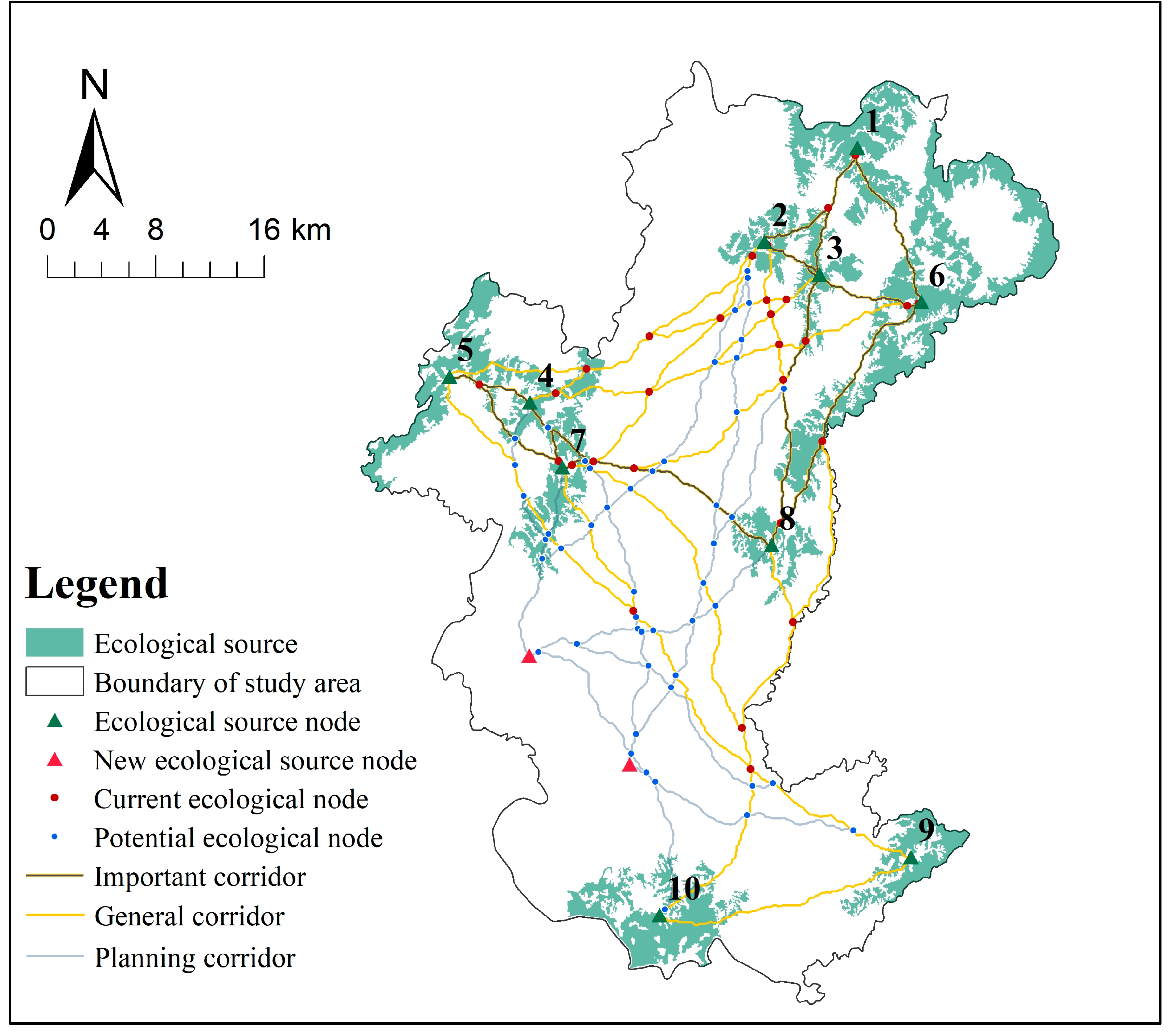
3.3.3. Optimized Ecological Network

After the optimization, the ecological source area increased by 1.67%, and the corridor length increased by 52.51%. As calculated by the network analysis method, indices α, β, and γ in ecological network 8 were 1.32, 3.0, and 1.20, respectively, with an increase of 0.22 (20%), 0.5 (20%), and 0.16 (15.4%), based on network 7b. Although the optimized indices α, β, and γ were not as good as the original network 7a, they improved on network 7b and maintained a cost ratio of 0.94. This indicates that the network structure connectivity has improved and is more economical to build than network 7a (see Table 9).

3.4. Exploration of Ecological Corridor Width

Figure 9 shows the results for the area occupied by each landscape type at different widths. As the width of the corridor increased, the area proportion of cultivated land and forestland fluctuated greatly, while the proportion of grassland, waters, and construction land fluctuated less. The area of forestland showed a decreasing trend; in contrast, the area proportion of cultivated land, grassland, waters, and construction land increased continuously. Despite the single fluctuation of the proportion, the decrease rate of the forest area share was the sharpest (4.77%) when the corridor width increased from 50 m to 100 m. For this reason, the width of the corridor should be limited to 50 m, taking into account the construction cost. Previous studies indicate that the corridor can meet the basic habitat requirements of small mammals, herbaceous plants, and most birds with a range of 30 m to 60 m [53]. In summary, the current construction of ecological corridors in Changsha County should be controlled in order to be within the range of 30 m to 50 m. This range, with more than 80% forestland, can play an important function in the spread and migration of species.

4. Discussion

4.1. Ecological Sources Characteristics and Assignment of Resistance Factors

The internal homogeneity and external expansiveness of the ecological sources make them suitable for species’ habitats [54]. So, the conservation of ecological sources is of great importance for biodiversity. The ecological sources in Changsha County are large and concentrated, particularly in the forestland of the northeastern part of the region. The marginal areas of the county have a smaller population distribution and forestland that has not been reclaimed; so, the ecological sources are more continuous. In contrast, in most city-level studies, the ecological sources were small and evenly distributed [52,55]. Highly urbanized areas have widely distributed populations and higher levels of fragmentation of forestland caused by human disturbance [56], resulting in this discrepancy.
Ten ecological sources were identified based on the CMSPACI method, and several of them coincided relatively well with the locations of the forest parks. However, the areas of these forest parks differed from the areas of the sources in which they were located. Notably, the Beishan Forest Park was not identified as an ecological source in its entirety. This suggests that even for those landscape types that are more suitable as habitats for species, CMSPACI can identify fragmented patches with little connectivity within them and can remove them from the scope of the ecological sources. This approach identifies ecological sources from the internal structure of the landscape, rather than exclusively from the landscape type; so, the results are more objective than those of direct identification.
Regional resistance is calculated based on the raster data of the nature–landscape–human activities, and the results focus more on the spatial characteristics of the practice area. The weight assignment of a resistance factor is an important link with which to accurately express the overall resistance of a region. Most of the previous studies on ecological resistance assignments used the analytic hierarchy process (AHP) [57,58,59]. However, this method is more subjective and does not consider the actual spatial situation of the region. The SPCA method in this paper is implemented by combining Arc GIS 10.8 tools and mathematical–statistical models to improve the weighting of the resistance factors. We found that the density of the road network in Changsha County accounted for the largest weight of the resistance surface. In contrast, the factor of the land cover type has had the greatest weight in many city-level studies [60,61]. This is because Changsha County, as the eastern gate of Changsha City, takes over several major highways that connect to the city. Meanwhile, Huanghua Airport, one of China’s twelve mainline airports, is located in Changsha County, resulting in a difference in traffic volume between urban areas and rural areas. This difference enhances the spatial heterogeneity of the road network density in Changsha County, making this spatial variable more volatile in terms of landscape connectivity. On the other hand, counties generally only have large areas of construction land where they are connected to urban areas. However, cities tend to have a polycentric development pattern [62], especially in highly urbanized areas [63]. Thus, at the municipal level, land cover is more disruptive to landscape connectivity. The study of ecological resistance at different study area scales depends on the actual spatial characteristics, and SPCA gives a feasible method for factor assignment.

4.2. Optimal Width of Ecological Corridors

Ecological corridors act as links to facilitate the flow of energy between ecological sources to maximize their benefits [64]. The definition of width gives a clear guideline range for the corridors and provides options for spatial planning. Guided by circuit theory, some scholars calculated the appropriate corridor width by calculating species dispersal distance [65,66]. However, balancing the contradiction between urban expansion and ecological conservation is the focus of sustainable economic development in the county. Therefore, land type, rather than specific species characteristics, should be considered when delineating corridor width. The appropriate ecological corridor widths delineated in this paper are 30 m to 50 m depending on the variation of land cover types occupied by the different buffer zones. However, land use needs to be guided on a case-by-case basis when conducting the spatial planning of ecological corridors.
The county is a place where towns and villages merge, and the focus of ecological corridor planning varies according to different regional characteristics. The rural areas in the northern part of the region have a large number of continuous ecological sources; so, the 30–50 m corridor range includes a large number of ecological spaces. As of 2022, several great crested grebes, a collared scops owl, an owlet, a falcon, and a white pheasant were rescued and released into the mountains in Chang-Zhu-Tan [67]. These birds are more likely to be found in corridors in the range of 25–50 m [68]. The more continuous ecological space in rural areas provides conditions for the habitats and migrations of such wild species. Therefore, in the northern part of the region, attention should be paid to the conservation of land cover types within the width of the corridor to ensure the continuity of species migration paths.
In the central part of the district, however, urbanization features are evident, with much of the land already occupied by construction land. With scarce land resources and expensive land prices, the construction of ecological corridors needs to be considered economical [69]. How to use the available resources to integrate the fragmented green spaces is the key issue. In key development areas where construction sites have been established, corridor construction can only be enhanced by restoring urban ecological spaces within the width. This means that traffic arteries intersecting with the corridor should ensure the greening rate of the road within the width. At the same time, road greening should be connected with different forms of landscape to form ecological corridors, such as pocket parks and urban wetlands. Cultivated land is the guarantee of crop cultivation in the region; so, it cannot be blindly returned to the forest. Low-intensity cultivated land has a high biodiversity at the edges and acts as an ecological space. Therefore, it is necessary to control the intensity of cropland reclamation within the corridor width of 30 m to 50 m.

4.3. Limitations of the Present Study

There are limitations to the study. First, the resistance factors were systematically selected from natural, landscape, and human aspects, avoiding the consideration of land use alone, as in previous studies. However, the resistance factors affecting regional energy flows can vary depending on regional characteristics, such as mining activity. A more detailed selection based on the study area characteristics should be developed to accurately determine the minimum resistance path in this region. Additionally, heterogeneity exists in the same type of landscape, and we can further consider the correction of land cover using nighttime lighting data or impervious surface data to make the resistance surface results more accurate. Second, we set a threshold of 1000 m when computing the landscape connectivity indices PC and dPC, but there is no unique statement about this threshold. Some scholars chose 1100 m, 1000 m, or 1400 m as thresholds when constructing the EN from 1990 to 2020 [70]. In the future studies, scholars should give further consideration to thresholds based on the dispersal distances of specific species within the study area. Finally, our study focuses on the construction and optimization of EN based on current land cover; hence, it is lacking in the ability to predict the future. So, different land cover scenarios should be simulated in the software to predict the future EN structure.

5. Conclusions

The construction of EN can improve landscape connectivity and enhance energy flow between regions. In this paper, we improved the method of constructing and optimizing EN in Changsha County. CMSPACI was used to identify ecological sources. Based on the SPCA method, the weight of each factor in the resistance surface was specified. The ecological corridors were determined with the MCR model and graded by the gravity model. In addition, the appropriate width of the ecological corridors was explored. The main conclusions are as follows:
  • From 2000 to 2020, the CA, NP, PD, and LPI of the construction land showed an increase, demonstrating the expansion of construction land. Forestland, cultivated land and grassland suffered fragmentation due to urbanization. Wetland occurrence in 2020 increased SHEI and SHDI. Wetlands integrate natural and man-made landscapes and can generate ecological value. In the future, it is important to focus on the construction and protection of urban wetlands in the central part of the region.
  • The 10 ecological sources extracted according to CMSPACI show regional heterogeneity. The ecological sources in the north were numerous, large, and continuous. Ecological source 6 had long edges, resulting in patches that were more vulnerable to external disturbance. The creation of buffer zones should be prioritized to protect the stability of the patches. The relative absence of ecological sources in the south and central regions reflects the lack of connectivity in these regions and the need for source optimization.
  • The results of the weight distribution of the resistance factors analyzed by the SPCA show that the density of the road network has the highest weight, demonstrating that roads are the main impediment to ecological processes. In urban areas with a dense road network, the focus should be on road greening to create green corridors.
  • A total of 25 existing corridors were extracted based on the MCR model, including 11 important corridors. The ecological corridors were mainly concentrated in the north and were mostly horizontal, and there were fewer longitudinal corridors. The north–south corridor runs through a high resistance area in the central region. As a result, the north–south corridors are prone to disruption, affecting the overall connectivity of the ecological network. In this paper, the EN was optimized with 2 new sources, 10 new corridors, 28 current ecological nodes, and 52 potential nodes. After optimization, the network connectivity was significantly improved.
  • The appropriate width of the ecological corridors in Changsha County is in the range of 30–50 m. The most effective means of balancing the urban expansion and ecological connectivity of Changsha County is to build an ecological network within this width. The arbitrary conversion of ecological land within the width to construction land should be prohibited, especially for the corridor running through the central part.

Author Contributions

Conceptualization, S.L. and Y.X.; methodology, S.L. and Y.X.; software, Y.X. and Y.J.; validation, Y.J. and J.Q.; formal analysis, Y.X.; investigation, S.L., Y.J., J.L. and J.Q.; resources, S.L.; data curation, J.L., H.S. and Y.C.; writing—original draft preparation, S.L.; writing—review and editing, S.L., Y.X. and W.L.; visualization, Y.J. and Y.Y.; supervision, S.L.; project administration, W.L.; funding acquisition, W.L. All authors have read and agreed to the published version of the manuscript.

Funding

This research was funded by the National Natural Science Foundation of China (NO. 52108049, NO. 42177072, and NO. 51909283), the Natural Science Foundation of Hunan Province, China (NO. 2020JJ4711 and NO. 2023JJ30182), the Humanities and Social Science Fund of Ministry of Education of China (NO. 20YJCZH003), the Key Research and Development Program of Hunan Province in China (NO. 2020WK2001), and the Fundamental Research Funds for the Central Universities of Central South University (NO. 2022XQLH155).

Data Availability Statement

The data presented in this study are available on request from the corresponding author.

Acknowledgments

Thanks to Central South University Human Settlements Research Center for the theoretical and methodological support.

Conflicts of Interest

The authors declare no conflict of interest.

Appendix A

Table A1. Eigenvalues and cumulative contribution of principal components.
ComponentsEigenvaluesContribution Rates (%)Accumulative Contribution Rate (%)
10.6302151.847551.8475
20.1788814.716366.5638
30.1568112.900879.4646
40.103978.553988.0184
50.087957.235495.2538
60.057694.7462100
1–6 indicate the number of spatial components extracted during the analysis. There are as many components extracted during principal component analysis as there are variables put into them. There were six resistance factor variables in this paper; so, six principal components were extracted. The principal component here did not represent the resistance factor. If the cumulative variance contribution rate of the current n principal components reaches a certain value (generally more than 80%), the first n principal components can be retained. So, we kept the first five principal components.
Table A2. Relationship matrix of principal components and evaluation indicators.
Evaluation IndicatorsComponents
12345
DEM−0.255560.076370.39711−0.00711−0.15202
Slope−0.285670.247470.773140.183160.22051
FVC0.48712−0.081480.11490.82362−0.2464
Land cover0.549520.614670.18022−0.39432−0.36129
Density of road network0.46614−0.664230.43222−0.351290.17498
NDBI0.31070.32751−0.109850.095750.84048

References

  1. Shi, W.; Tian, J.; Namaiti, A.; Xing, X. Spatial-Temporal Evolution and Driving Factors of the Coupling Coordination between Urbanization and Urban Resilience: A Case Study of the 167 Counties in Hebei Province. Int. J. Environ. Res. Public Health 2022, 19, 27. [Google Scholar] [CrossRef]
  2. Lv, Z.Q.; Wu, Z.F.; Wei, J.B.; Sun, C.; Zhou, Q.G.; Zhang, J.H. Monitoring of the urban sprawl using geoprocessing tools in the Shenzhen Municipality, China. Environ. Earth Sci. 2011, 62, 1131–1141. [Google Scholar] [CrossRef]
  3. Su, S.L.; Jiang, Z.L.; Zhang, Q.; Zhang, Y.A. Transformation of agricultural landscapes under rapid urbanization: A threat to sustainability in Hang-Jia-Hu region, China. Appl. Geogr. 2011, 31, 439–449. [Google Scholar] [CrossRef]
  4. Zhang, J.; Qu, M.; Wang, C.; Zhao, J.; Cao, Y. Quantifying landscape pattern and ecosystem service value changes: A case study at the county level in the Chinese Loess Plateau. Glob. Ecol. Conserv. 2020, 23, 14. [Google Scholar] [CrossRef]
  5. Huang, K.; Peng, L.; Wang, X.; Deng, W. Integrating circuit theory and landscape pattern index to identify and optimize ecological networks: A case study of the Sichuan Basin, China. Environ. Sci. Pollut. Res. 2022, 29, 66874–66887. [Google Scholar] [CrossRef]
  6. Huo, J.G.; Shi, Z.Q.; Zhu, W.B.; Li, T.Q.; Xue, H.; Chen, X.; Yan, Y.H.; Ma, R. Construction and Optimization of an Ecological Network in Zhengzhou Metropolitan Area, China. Int. J. Environ. Res. Public Health 2022, 19, 20. [Google Scholar] [CrossRef] [PubMed]
  7. Jalkanen, J.; Toivonen, T.; Moilanen, A. Identification of ecological networks for land-use planning with spatial conservation prioritization. Landsc. Ecol. 2020, 35, 353–371. [Google Scholar] [CrossRef] [Green Version]
  8. Tian, M.R.; Chen, X.L.; Gao, J.X.; Tian, Y.X. Identifying ecological corridors for the Chinese ecological conservation redline. PLoS ONE 2022, 17, e0271076. [Google Scholar] [CrossRef]
  9. Park, S.C.; Han, B.H. Using the City Biodiversity Index as a Method to Protect Biodiversity in Korean Cities. Sustainability 2021, 13, 11284. [Google Scholar] [CrossRef]
  10. Chapman, C.; Hall, J.W. Designing green infrastructure and sustainable drainage systems in urban development to achieve multiple ecosystem benefits. Sustain. Cities Soc. 2022, 85, 104078. [Google Scholar] [CrossRef]
  11. Fonseca, A.; Zina, V.; Duarte, G.; Aguiar, F.C.; Rodriguez-Gonzalez, P.M.; Ferreira, M.T.; Fernandes, M.R. Riparian Ecological Infrastructures: Potential for Biodiversity-Related Ecosystem Services in Mediterranean Human-Dominated Landscapes. Sustainability 2021, 13, 10508. [Google Scholar] [CrossRef]
  12. Wang, X.; Sun, Y.J.; Liu, Q.H.; Zhang, L.G. Construction and Optimization of Ecological Network Based on Landscape Ecological Risk Assessment: A Case Study in Jinan. Land 2023, 12, 743. [Google Scholar] [CrossRef]
  13. Zhao, Y.Y.; Kasimu, A.; Liang, H.W.; Reheman, R. Construction and Restoration of Landscape Ecological Network in Urumqi City Based on Landscape Ecological Risk Assessment. Sustainability 2022, 14, 8154. [Google Scholar] [CrossRef]
  14. Chen, Y.P.; Zheng, B.H.; Liu, R.J. The Evolution of Ecological Space in an Urban Agglomeration Based on a Suitability Evaluation and Cellular Automata Simulation. Sustainability 2022, 14, 7455. [Google Scholar] [CrossRef]
  15. Bai, H.; Li, Z.W.; Guo, H.L.; Chen, H.P.; Luo, P.P. Urban Green Space Planning Based on Remote Sensing and Geographic Information Systems. Remote Sens. 2022, 14, 4213. [Google Scholar] [CrossRef]
  16. Ran, Y.J.; Lei, D.M.; Li, J.; Gao, L.P.; Mo, J.X.; Liu, X. Identification of crucial areas of territorial ecological restoration based on ecological security pattern: A case study of the central Yunnan urban agglomeration, China. Ecol. Indic. 2022, 143, 109318. [Google Scholar] [CrossRef]
  17. Jiang, H.; Peng, J.; Zhao, Y.N.; Xu, D.M.; Dong, J.Q. Zoning for ecosystem restoration based on ecological network in mountainous region. Ecol. Indic. 2022, 142, 9. [Google Scholar] [CrossRef]
  18. Biondi, E.; Casavecchia, S.; Pesaresi, S.; Zivkovic, L. Natura 2000 and the Pan-European Ecological Network: A new methodology for data integration. Biodivers. Conserv. 2012, 21, 1741–1754. [Google Scholar] [CrossRef]
  19. Dai, L.; Liu, Y.; Luo, X. Integrating the MCR and DOI models to construct an ecological security network for the urban agglomeration around Poyang Lake, China. Sci. Total Environ. 2021, 754, 141868. [Google Scholar] [CrossRef] [PubMed]
  20. Yan, L.B.; Yu, L.F.; Zhou, C.W.; Yang, R. Study on functional division optimizing of Kuankuoshui national nature reserve based on resistance surface analysis. Bulg. Chem. Commun. 2017, 49, 140–143. [Google Scholar]
  21. Jia, Z.-Y.; Chen, C.-D.; Tong, X.-X.; Wu, S.-J.; Zhou, W.-Z. Developing and optimizing ecological networks for the towns along the Three Gorges Reservoir: A case of Kaizhou New Town, Chongqing. Shengtaixue Zazhi 2017, 36, 782–791. [Google Scholar] [CrossRef]
  22. Yang, C.H.; Guo, H.J.; Huang, X.Y.; Wang, Y.X.; Li, X.N.; Cui, X.Y. Ecological Network Construction of a National Park Based on MSPA and MCR Models: An Example of the Proposed National Parks of “Ailaoshan-Wuliangshan” in China. Land 2022, 11, 17. [Google Scholar] [CrossRef]
  23. Wang, S.; Wu, M.Q.; Hu, M.M.; Fan, C.; Wang, T.; Xia, B.C. Promoting landscape connectivity of highly urbanized area: An ecological network approach. Ecol. Indic. 2021, 125, 12. [Google Scholar] [CrossRef]
  24. Modica, G.; Pratico, S.; Laudari, L.; Ledda, A.; Di Fazio, S.; De Montis, A. Implementation of multispecies ecological networks at the regional scale: Analysis and multi-temporal assessment. J. Environ. Manag. 2021, 289, 18. [Google Scholar] [CrossRef]
  25. Ma, B.B.; Chen, Z.A.; Wei, X.J.; Li, X.Q.; Zhang, L.T. Comparative ecological network pattern analysis: A case of Nanchang. Environ. Sci. Pollut. Res. 2022, 29, 37423–37434. [Google Scholar] [CrossRef]
  26. Wang, Y.J.; Qu, Z.; Zhong, Q.C.; Zhang, Q.P.; Zhang, L.; Zhang, R.; Yi, Y.; Zhang, G.L.; Li, X.C.; Liu, J. Delimitation of ecological corridors in a highly urbanizing region based on circuit theory and MSPA. Ecol. Indic. 2022, 142, 17. [Google Scholar] [CrossRef]
  27. Wei, H.; Zhu, H.; Chen, J.; Jiao, H.Y.; Li, P.H.; Xiong, L.Y. Construction and Optimization of Ecological Security Pattern in the Loess Plateau of China Based on the Minimum Cumulative Resistance (MCR) Model. Remote Sens. 2022, 14, 5906. [Google Scholar] [CrossRef]
  28. Huang, C.; Hou, X.; Li, H. An improved minimum cumulative resistance model for risk assessment of agricultural non-point source pollution in the coastal zone. Environ. Pollut. (Barking, Essex: 1987) 2022, 312, 120036. [Google Scholar] [CrossRef] [PubMed]
  29. Zhai, T.L.; Huang, L.Y. Linking MSPA and Circuit Theory to Identify the Spatial Range of Ecological Networks and Its Priority Areas for Conservation and Restoration in Urban Agglomeration. Front. Ecol. Evol. 2022, 10, 16. [Google Scholar] [CrossRef]
  30. Chen, X.L.; Li, J.; Xu, L.Y. Ecological Extension of Regulatory Planning in China’s Territorial Spatial Planning System: A Case Study on Mentougou District, Beijing. Landsc. Archit. Front. 2020, 8, 42–55. [Google Scholar] [CrossRef]
  31. Jiao, H.F.; Zhang, X.X.; Yang, C.; Cao, X.Z. The characteristics of spatial expansion and driving forces of land urbanization in counties in central China: A case study of Feixi county in Hefei city. PLoS ONE 2021, 16, e0252331. [Google Scholar] [CrossRef]
  32. Zheng, L.; Wang, Y.; Li, J. Quantifying the spatial impact of landscape fragmentation on habitat quality: A multi-temporal dimensional comparison between the Yangtze River Economic Belt and Yellow River Basin of China. Land Use Policy 2023, 125, 106463. [Google Scholar] [CrossRef]
  33. Liang, C.; Zeng, J.; Zhang, R.C.; Wang, Q.W. Connecting urban area with rural hinterland: A stepwise ecological security network construction approach in the urban-rural fringe. Ecol. Indic. 2022, 138, 108794. [Google Scholar] [CrossRef]
  34. Lu, C.; Shi, L.; Fu, L.; Liu, S.; Li, J.; Mo, Z. Urban Ecological Environment Quality Evaluation and Territorial Spatial Planning Response: Application to Changsha, Central China. Int. J. Environ. Res. Public Health 2023, 20, 3753. [Google Scholar] [CrossRef] [PubMed]
  35. Ji, S.Y.; Choi, J.; Lee, S.H.; Lee, P.S.H. Prediction of Fragmentation Impact Range of Forest Development Analyzing the Pattern of Landscape Indexes. J. Korea Soc. Environ. Restor. Technol. 2016, 19, 109–119. [Google Scholar] [CrossRef]
  36. Zhang, L.-L.; Shi, Y.-F.; Liu, Y.-H. Effects of spatial grain change on the landscape pattern indices in Yimeng Mountain area of Shandong Province, East China. Shengtaixue Zazhi 2013, 32, 459–464. [Google Scholar]
  37. Zhang, L.; Hou, G.L.; Li, F.P. Dynamics of landscape pattern and connectivity of wetlands in western Jilin Province, China. Environ. Dev. Sustain. 2020, 22, 2517–2528. [Google Scholar] [CrossRef]
  38. Nie, W.B.; Shi, Y.; Siaw, M.J.; Yang, F.; Wu, R.W.; Wu, X.; Zheng, X.Y.; Bao, Z.Y. Constructing and optimizing ecological network at county and town Scale: The case of Anji County, China. Ecol. Indic. 2021, 132, 14. [Google Scholar] [CrossRef]
  39. An, Y.; Liu, S.; Sun, Y.; Shi, F.; Beazley, R. Construction and optimization of an ecological network based on morphological spatial pattern analysis and circuit theory. Landsc. Ecol. 2021, 36, 2059–2076. [Google Scholar] [CrossRef]
  40. Li, H.; Guo, W.Q.; Liu, Y.; Zhang, Q.M.; Xu, Q.; Wang, S.T.; Huang, X.; Xu, K.X.; Wang, J.Z.; Huang, Y.L.; et al. The Delineation and Ecological Connectivity of the Three Parallel Rivers Natural World Heritage Site. Biology-Basel 2023, 12, 3. [Google Scholar] [CrossRef]
  41. Hashemi, R.; Darabi, H. The Review of Ecological Network Indicators in Graph Theory Context: 2014–2021. Int. J. Environ. Res. 2022, 16, 24. [Google Scholar] [CrossRef]
  42. Yang, R.L.; Bai, Z.K.; Shi, Z.Y. Linking Morphological Spatial Pattern Analysis and Circuit Theory to Identify Ecological Security Pattern in the Loess Plateau: Taking Shuozhou City as an Example. Land 2021, 10, 907. [Google Scholar] [CrossRef]
  43. Huang, X.X.; Wang, H.J.; Shan, L.Y.; Xiao, F.T. Constructing and optimizing urban ecological network in the context of rapid urbanization for improving landscape connectivity. Ecol. Indic. 2021, 132, 108319. [Google Scholar] [CrossRef]
  44. Li, Z.; Ding, Y.; Wang, Y.-L.; Chen, J.; Wu, F.-M. Construction of Ecological Security Pattern in Mountain Rocky Desertification Area Based on MCR Model: A Case Study of Nanchuan, Chongqing. J. Ecol. Rural. Environ. 2020, 36, 1046–1054. [Google Scholar] [CrossRef]
  45. Zhang, S.Q.; Yang, P.; Xia, J.; Qi, K.L.; Wang, W.Y.; Cai, W.; Chen, N.C. Research and Analysis of Ecological Environment Quality in the Middle Reaches of the Yangtze River Basin between 2000 and 2019. Remote Sens. 2021, 13, 4475. [Google Scholar] [CrossRef]
  46. Li, Z.H.; Jiao, L.M.; Zhang, B.E.; Xu, G.; Liu, J.F. Understanding the pattern and mechanism of spatial concentration of urban land use, population and economic activities: A case study in Wuhan, China. Geo-Spat. Inf. Sci. 2021, 24, 678–694. [Google Scholar] [CrossRef]
  47. Chang, Y.; Hou, K.; Wu, Y.P.; Li, X.X.; Zhang, J.L. A conceptual framework for establishing the index system of ecological environment evaluation-A case study of the upper Hanjiang River, China. Ecol. Indic. 2019, 107, 11. [Google Scholar] [CrossRef]
  48. Xu, W.X.; Wang, J.M.; Zhang, M.; Li, S.J. Construction of landscape ecological network based on landscape ecological risk assessment in a large-scale opencast coal mine area. J. Clean Prod. 2021, 286, 11. [Google Scholar] [CrossRef]
  49. Kong, F.H.; Yin, H.W.; Nakagoshi, N.; Zong, Y.G. Urban green space network development for biodiversity conservation: Identification based on graph theory and gravity modeling. Landsc. Urban Plan. 2010, 95, 16–27. [Google Scholar] [CrossRef]
  50. Fu, B.; Liu, J.; Zhang, J.; Wu, X.; Wang, J. Service accessibility of ecological nodes: An exploratory way to enhance network connectivity in a study case of Wu’an, China. Ecol. Inform. 2022, 69, 101589. [Google Scholar] [CrossRef]
  51. Shen, Q.-W.; Lin, M.-L.; Mo, H.-P.; Huang, Y.-B.; Hu, X.-Y.; Wei, L.-W.; Zheng, Y.-S.; Lu, D.-F. Ecological network construction and optimization in Foshan City, China. Yingyong Shengtai Xuebao 2021, 32, 3288–3298. [Google Scholar] [CrossRef] [PubMed]
  52. Zhao, S.M.; Ma, Y.F.; Wang, J.L.; You, X.Y. Landscape pattern analysis and ecological network planning of Tianjin City. Urban For. Urban Green. 2019, 46, 12. [Google Scholar] [CrossRef]
  53. Yang, Z.G.; Jiang, Z.Y.; Guo, C.X.; Yang, X.J.; Xu, X.J.; Li, X.; Hu, Z.M.; Zhou, H.Y. Construction of ecological network using morphological spatial pattern analysis and minimal cumulative resistance models in Guangzhou City, China. Yingyong Shengtai Xuebao = J. Appl. Ecol. 2018, 29, 3367–3376. [Google Scholar] [CrossRef]
  54. Shi, N.-N.; Han, Y.; Wang, Q.; Quan, Z.-J.; Luo, Z.-L.; Ge, J.-S.; Han, R.-Y.; Xiao, N.-W. Construction and optimization of ecological network for protected areas in Qinghai Province. Shengtaixue Zazhi 2018, 37, 1910–1916. [Google Scholar] [CrossRef]
  55. Guo, N.A.; Liang, X.B.; Meng, L.R. Evaluation of the Thermal Environmental Effects of Urban Ecological Networks-A Case Study of Xuzhou City, China. Sustainability 2022, 14, 7744. [Google Scholar] [CrossRef]
  56. Fahey, R.T.; Casali, M. Distribution of forest ecosystems over two centuries in a highly urbanized landscape. Landsc. Urban Plan. 2017, 164, 13–24. [Google Scholar] [CrossRef] [Green Version]
  57. Chen, X.J.; Chen, S.B.; He, Z.W.; Xue, D.J.; Fang, G.Z.; Pan, K.W.; Fang, K. Developing a system for comprehensive regional Eco-environmental quality assessment in mountainous areas—A case study of Western Sichuan, China. Front. Environ. Sci. 2022, 10, 1325. [Google Scholar] [CrossRef]
  58. Li, Z.M.; Fan, Z.X.; Shen, S.G. Urban Green Space Suitability Evaluation Based on the AHP-CV Combined Weight Method: A Case Study of Fuping County, China. Sustainability 2018, 10, 2656. [Google Scholar] [CrossRef] [Green Version]
  59. Hou, K.; Li, X.X.; Wang, J.J.; Zhang, J. Evaluating Ecological Vulnerability Using the GIS and Analytic Hierarchy Process (AHP) Method in Yan‘an, China. Pol. J. Environ. Stud. 2016, 25, 599–605. [Google Scholar]
  60. Zhang, C.X.; Jia, C.; Gao, H.G.; Shen, S.G. Ecological Security Pattern Construction in Hilly Areas Based on SPCA and MCR: A Case Study of Nanchong City, China. Sustainability 2022, 14, 21. [Google Scholar] [CrossRef]
  61. Li, Y.Y.; Zhang, Y.Z.; Jiang, Z.Y.; Guo, C.X.; Zhao, M.Y.; Yang, Z.G.; Guo, M.Y.; Wu, B.Y.; Chen, Q.L. Integrating morphological spatial pattern analysis and the minimal cumulative resistance model to optimize urban ecological networks: A case study in Shenzhen City, China. Ecol. Process. 2021, 10, 15. [Google Scholar] [CrossRef]
  62. Liu, X.J.; Derudder, B.; Wang, M.S. Polycentric urban development in China: A multi-scale analysis. Environ. Plan. B-Urban Anal. City Sci. 2018, 45, 953–972. [Google Scholar] [CrossRef]
  63. Yang, Z.W.; Chen, Y.B.; Zheng, Z.H.; Wu, Z.F. Identifying China’s polycentric cities and evaluating the urban centre development level using Luojia-1A night-time light data. Ann. Gis 2022, 28, 185–195. [Google Scholar] [CrossRef]
  64. Liu, Z.Y.; Gan, X.Y.; Dai, W.N.; Huang, Y. Construction of an Ecological Security Pattern and the Evaluation of Corridor Priority Based on ESV and the “Importance-Connectivity” Index: A Case Study of Sichuan Province, China. Sustainability 2022, 14, 3985. [Google Scholar] [CrossRef]
  65. Wei, J.Q.; Zhang, Y.; Liu, Y.; Li, C.; Tian, Y.S.; Qian, J.; Gao, Y.; Hong, Y.S.; Liu, Y.F. The impact of different road grades on ecological networks in a mega-city Wuhan City, China. Ecol. Indic. 2022, 137, 108784. [Google Scholar] [CrossRef]
  66. Li, Y.; Peng, Y.X.; Li, H.L.; Zhu, W.H.; Darman, Y.; Lee, D.K.; Wang, T.M.; Sedash, G.; Pandey, P.; Borzee, A.; et al. Prediction of range expansion and estimation of dispersal routes of water deer (Hydropotes inermis) in the transboundary region between China, the Russian Far East and the Korean Peninsula. PLoS ONE 2022, 17, e0264660. [Google Scholar] [CrossRef] [PubMed]
  67. Bureau, H.P.F. Look! Fantastic animals make their home in Changsha. 2023. Available online: https://new.qq.com/rain/a/20230213A09O1100.
  68. Shen, J.K.; Wang, Y.C. An improved method for the identification and setting of ecological corridors in urbanized areas. Urban Ecosyst. 2022, 26, 141–160. [Google Scholar] [CrossRef]
  69. Xie, Y.S.; Wang, Q.N.; Xie, M.Q.; Shibata, S. Construction feasibility evaluation for potential ecological corridors under different widths: A case study of Chengdu in China. Landsc. Ecol. Eng. 2023, 19, 381–399. [Google Scholar] [CrossRef]
  70. Xie, J.; Xie, B.G.; Zhou, K.C.; Li, J.H.; Xiao, J.Y.; Liu, C.C. Impacts of landscape pattern on ecological network evolution in Changsha-Zhuzhou-Xiangtan Urban Agglomeration, China. Ecol. Indic. 2022, 145, 109716. [Google Scholar] [CrossRef]
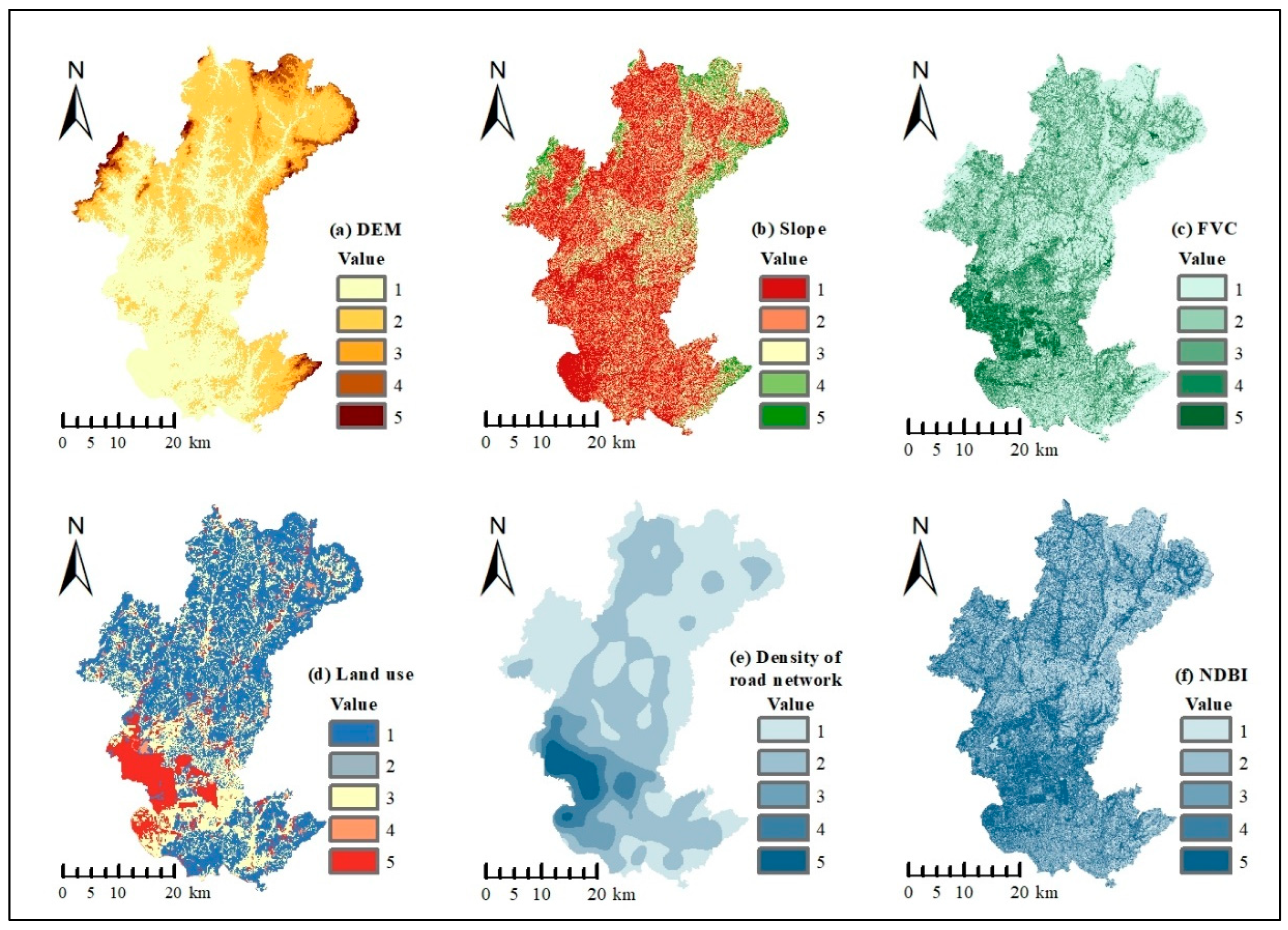
Figure 1. Location of the study area.
Land 12 01379 g001
Figure 2. Morphological spatial pattern analysis result.
Land 12 01379 g002
Figure 3. Classification of resistance factor.
Land 12 01379 g003
Figure 4. 2000–2020 Land cover change.
Land 12 01379 g004
Figure 5. Distribution of ecological sources.
Land 12 01379 g005
Figure 6. Comprehensive resistance surface grading.
Land 12 01379 g006
Figure 7. Ecological network map.
Land 12 01379 g007
Figure 8. Optimized ecological network.
Land 12 01379 g008
Figure 9. Percentage of land type area occupied by ecological corridors at different widths.
Land 12 01379 g009
Table 1. Resistance factors scoring system.
Index Type Rate LevelRate Criteria
Natural conditionsDEM (m)1<68
268~114
3114~194
4194~316
5316~636
Slope (°)1<4.64
24.64~8.91
38.91~14.91
414.91~23.24
523.24~49.39
FVC10.87~1
20.72~0.87
30.55~0.72
40.35~0.55
50~0.35
Landscape
Type
Land cover1Forestland or grassland
2Wetland
3Cultivated land
4Waters
5Construction land
Human disturbanceDensity of road network (km/km2)10~0.60
20.60~1.65
31.65~3.23
43.23~5.11
55.11~8.10
NDBI1−0.96~−0.33
2−0.33~−0.23
3−0.23~−0.13
4−0.13~−0.04
5−0.04~0.49
Table 2. Principal component loading matrix and weight assignment.
IndexComponents
12345Weight
DEM−0.321920.1805681.002822−0.02205−0.632920.05
Slope−0.359850.5851161.9524110.5680370.743550.13
FVC0.613611−0.192650.2901572.554306−0.830850.19
Land cover0.6922151.453320.45511−1.22291−1.218250.18
Density of road network1.571804−1.57051.091486−1.089460.5900250.24
NDBI0.391380.774361−0.27740.2969512.8340630.20
Table 3. Class level indices in 2000, 2010, 2020.
YearLand CoverLandscape Indices
CANPPDLPIEDSPLIT
2000Cultivated land58,457.7948702.7715.9095.3536.34
Forestland10,2351.418,49810.5317.93108.0621.48
Grassland10,362.5119,05010.840.1137.02278,873.11
Waters1673.643740.210.062.57571,426.94
Construction land2902.14810.050.671.4021,263.28
2010Cultivated land56,585.4345812.6114.1293.2542.44
Forestland102,913.218,81310.7017.96109.3121.36
Grassland10,465.5619,04910.840.1137.28269,502.17
Waters1368.813940.220.082.63538,401.68
Construction land4414.51580.091.413.604951.10
2020Cultivated land51,873.6645212.577.0876.66128.65
Forestland93,479.2212,5807.1617.5088.0324.38
Grassland8947.4416,3839.320.1431.32196,161.31
Wetlands26.2830.010.010.0285,023,213.94
Waters2528.463300.190.152.94105,310.19
Construction land18,893.794730.275.927.36276.36
Table 4. Landscape level indices in 2000, 2010, 2020.
YearLandscape Metrics
CONTAGSPLITSHDISHEI
200052.624713.48910.960.5965
201051.78214.16870.97660.6068
202053.399519.07351.14960.6416
Table 5. Statistics of landscape types based on MSPA.
Landscape TypeArea/km2Proportion of Area of Prospect Data (%)Proportion of Area of County (%)
Core710.30 69.33%40.42%
Islet30.88 3.01%1.76%
Perforation17.96 1.75%1.02%
Edge175.53 17.13%9.99%
Loop21.20 2.07%1.21%
Bridge27.70 2.70%1.58%
Branch40.95 4.00%2.33%
Total1024.53 100.00%58.30%
Table 6. Ecological source area and landscape connectivity index.
NumberArea/km2dPC
691.194337.19752
728.94426.82195
139.63615.56345
531.06810.74489
814.813110.39394
315.90487.153005
213.14637.072748
410.06296.659909
1039.61172.63524
920.53352.237005
Table 7. Percentage of area of each resistance.
Resistance LevelHighMid-HighMidMid-LowLow
Area (km2)13.9726.2441.8148.7943.84
Proportion (%)8.0015.123.927.925.1
Table 8. Interaction intensity matrix between ecological sources according to gravity model.
Sources Number12345678910
100.406 0.567 0.042 0.029 0.397 0.042 0.070 0.009 0.011
2 01.462 0.072 0.044 0.296 0.070 0.097 0.009 0.011
3 00.071 0.044 1.045 0.075 0.162 0.012 0.014
4 00.764 0.054 1.271 0.107 0.010 0.013
5 00.035 0.266 0.058 0.008 0.010
6 00.058 0.145 0.013 0.015
7 00.165 0.012 0.015
8 00.022 0.028
9 00.087
10 0
Table 9. Network structure index comparison.
Network 7aNetwork 7bNetwork 8
A2.41.11.32
Β4.52.53.0
Γ1.871.041.20
C0.960.940.94
Disclaimer/Publisher’s Note: The statements, opinions and data contained in all publications are solely those of the individual author(s) and contributor(s) and not of MDPI and/or the editor(s). MDPI and/or the editor(s) disclaim responsibility for any injury to people or property resulting from any ideas, methods, instructions or products referred to in the content.

