Ecosystem Service Optimisation in the Central Plains Urban Agglomeration Based on Land Use Structure Adjustment

Abstract

By using the methods of scenario analysis, model simulation, and the multi-objective spatial optimisation algorithm Non-dominated Sorting Genetic Algorithm-II (NSGA-II), the Pareto optimal solutions for water supply, water purification (N retention), as well as carbon storage and sequestration service (carbon service) of the Central Plains Urban Agglomeration (CPUA) were sought by adjusting the land use structure. It showed that, to reach the Pareto optimal solution goal, (1) in Scenario 1 (S1), the water supply service needs to increase by 10.682 billion cubic metres, the water purification (N retention) service needs to decrease by 11,400 tons, and the carbon service need to decrease by 2.487 billion tons. In Scenario 2 (S2), the water supply service needs to increase by 8.243 billion cubic metres, the water purification (N retention) service needs to decrease by 11,000 tons, and the carbon service needs to decrease by 2.466 billion tons. In Scenario 3 (S3), the water supply service needs to increase by 4.089 billion cubic metres, the water purification (N retention) service needs to decrease by 10,800 tons, and the carbon service needs to decrease by 2.380 billion tons. (2) After land use optimisation and adjustment, the S3 ecological land structure is complete and consistent with the vision of ecological protection and urban development in the study area, which is the optimal scenario. (3) Optimising the ecosystem service supply pattern through land use structure adjustment could balance the overall ecosystem service supply pattern of the study area In regions wherein ecosystem supply is insufficient and there is a spatial mismatch between supply and demand for ecosystem services, this study can guide regional land planning and assist in the formulation of ecosystem service management policies.

1. Introduction

The ecosystem provides various service functions (supply, regulation, support, and cultural services) in terms of natural resources and living environments for humans, and humans provide demand and consumption for its products and services [1,2]. Human society depends on ecosystem services to survive, and both supply and demand constitute a dynamic process of ecosystem services flowing from the natural ecosystem to the human social system [3]. Therefore, ecosystem services represent the core of human utilisation [4]. Some studies have examined ecosystem services’ supply potential, demand, and supply and demand matching [5,6]. They have found that, only when the supply of ecosystem services matches people’s demand can the management of ecosystem services play a large role in social and economic development [7,8,9,10].

Pareto frontiers have been widely used in determining the goals of ecosystem service optimisation, which aims to pursue the Pareto optimal solution for ecosystem service [10,11]. Aiming for a Pareto optimal solution, the idea of ecosystem service optimisation is as follows: [9] A series of land use situations under different management objectives of protection and development are set up, and the optimal ecosystem service combination (Pareto curve) and corresponding land use planning scheme are obtained using the optimisation model. Then, land use optimisation under the guidance of ecosystem services is conducted, and the land use type transformation is implemented quantitatively and systematically to seek the optimal land use pattern under an optimal ecosystem service [12,13,14].

Regarding method application, the optimisation of ecosystem services is often realised by integrating biophysical and mathematical optimisation models [15]. Among them, InVEST (Integrated Valuation of Ecosystem Services and Tradeoffs) is the commonly used biophysical model, and the multi-objective spatial optimisation algorithm Non-dominated Sorting Genetic Algorithm-II (NSGA-II) is the most commonly used mathematical model. For example, Lautenbach et al. integrated the SWAT and NSGA-II models to study the effects of different crop-planting patterns on food supply, water yield, biofuel, and water purification, obtaining the optimal set of ecosystem services [16,17]. Hu et al. developed the SAORES ecosystem services optimisation model, which integrated the InVEST and NSGA-II models, to study the impact of land use structure change on water yield, soil conservation, carbon storage, and food production. They then optimised the ecosystem services with trade-off relations, achieving good optimisation results [17].

The NSGA-II algorithm is the most efficient calculation method with a multi-objective function, which is mainly used to simulate a series of land use schemes and obtain the Pareto optimal set of ecosystem services. With the Pareto optimal set as the primary data, Python language or statistical software is used to complete data visualisation, drawing the Pareto curve and displaying the optimisation results [10]. Currently, the NSGA-II algorithm is mature for applying ecosystem service optimisation. However, it still has the following deficiencies: When optimising the setting of constraint conditions, more attention is paid to the possible spatial layout of land use, but less attention is paid to the constraint conditions of ecosystem services. It is also necessary to set the threshold value of ecosystem services in combination with the supply–demand relationship and matching characteristics and improve the service constraints to improve the accuracy and applicability of the optimisation results.

Urban agglomerations are “urban clusters” formed by several densely distributed cities and their hinterlands through spatial interaction based on certain natural environmental conditions and regional network organisation. Their essence is to maximise the scale effect and linkage effect of urban agglomerations through close connections and collaborative interactions among cities [18,19]. Natural ecosystem services provide a variety of service functions (supply service, regulation service, support service, and cultural service) for human beings to meet their demands for products and services, and both the supply and demand parties jointly complete the dynamic process of ecosystem services flowing from natural ecosystem to human social system [20]. As a bridge linking the natural ecosystem and the socio-economic system [6,9,21], ecosystem services serve as a link for the material and energy exchange between the natural ecosystem and the socio-economic system, and provide the material and environmental foundation for the socio-economic development of urban agglomerations [9,22]. Optimising the supply and demand structure of ecosystem services in urban agglomerations and implementing integrated ecological service management have become important ways to optimise the interdependence of urban agglomerations [4,20,23], which can prompt urban agglomerations to constantly adapt to the natural ecological environment and ultimately achieve sustainable social and economic development [4,24]. At present, China’s Yangtze River Delta urban agglomerations [25] and the Beijing–Tianjin–Hebei urban agglomerations [26] have carried out a significant amount of beneficial exploration in related fields and achieved many positive results, providing useful references for other urban agglomerations.

As some of the urban agglomerations in central and western China that are severely constrained by resources and the environment, rapid urbanisation and population agglomeration have caused tremendous pressure on the regional ecological environment, and problems such as water environment pollution and water resource shortage in some areas have become increasingly serious [27]. Integrating the demand for ecosystem services into space management, optimising and adjusting the supply structure of ecosystem services, and matching the supply and demand of ecosystem services are the primary issues to be considered in solving the ecological dilemma of the CPUA. Taking the CPUA as an example, this project explores the optimisation of urban agglomeration ecosystem services based on supply and demand matching, which enriches the research content related to the optimisation of urban agglomeration ecosystem services and helps people to establish “large region” and “environment” perspectives, providing theoretical guidance for coordinated natural, social, and economic development between regions.

2. Materials and Methods

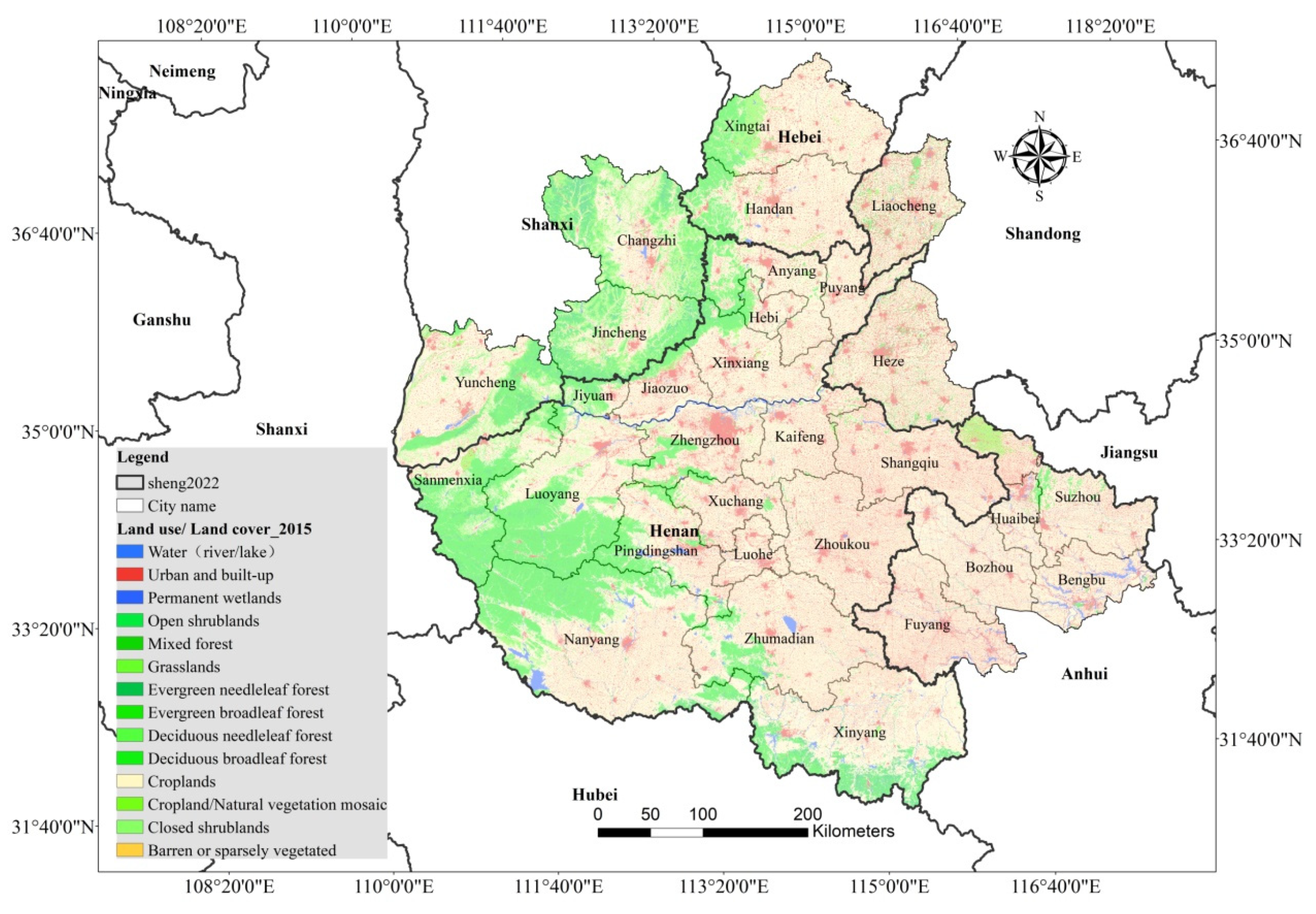
2.1. Study Area

Located in central and western China, the CPUA covers an area of 287,000 square kilometres, including 30 prefecture-level cities in the Henan, Shandong, Shanxi, Shaanxi, and Anhui provinces (Figure 1). With Zhengzhou as the core city, it covers the whole Henan province. The population and economic activities of the CPUA are highly intensive, and the regional ecological resources are rich. However, the spatial distribution of socioeconomic and ecological resources is very uneven. The ecological resources are mainly distributed in the ecological space composed of the Liankang Mountains, Funiu Mountains, Taihang Mountains, the ecological corridors along the middle line of the South-to-North Water Diversion Project, and the middle and lower reaches of the Yellow River. Socioeconomic activities are mainly concentrated in the urban space in the central and eastern regions [28].

With the continuous intensive development of urban agglomerations, the flow of ecosystem services is more frequent and concentrated, and the difference between the supply and demand of ecosystem services between regions is gradually increasing. The degradation of the regional ecosystem service’s supply function, water resource shortages, water environment pollution, and increased carbon emission have become major limiting factors for the healthy and sustainable development of the CPUA [27]. In this context, it is vital to realise ecosystem service management and optimise ecosystem services to match their supply and demand. This research can provide spatial guidance for realising the objectives of ecosystem service management.

2.2. Materials

The land use data used in this paper are based on the Landsat remote sensing image of the United States as the primary information source and the national scale multi-period land use/land cover thematic database of China constructed by artificial visual interpretation. This paper uses land use data for the study area from 2010, 2015, and 2020. Spatial distribution data of China’s altitude (digital elevation model) are derived from the Shuttle Radar Topography Mission (SRTM) data of the US Space Shuttle Endeavour and based on the 30 m provincial data generated in the recent SRTM V4.1 update. The data were projected using the WGS84 ellipsoid. Meteorological observation data were obtained from the China Meteorological Data network (http://data.cma.cn/, accessed on 16 May 2021). In this study, potential evaporation, daily precipitation, and other meteorological data from meteorological stations in the CPUA in 2015 were selected and processed to obtain the meteorological data for the study area. The Soil Data with a resolution of 1000 m is derived from China Soil Dataset at www.resdc.cn (accessed on 16 May 2021). The spatial population distribution data refers to the statistical population data of districts and counties. Considering the population distribution influencing factors such as land use type, night light brightness, and residential density, the multi-year population distribution grid data were prepared through spatialisation with a spatial resolution of 1000 m. The above remote sensing and spatial data can be accessed at www.resdc.cn (accessed on 16 May 2021).

The reference standards for water quota and water purification requirements used in this study refer to the environmental capacity issued by local governments in the study area [29]. Per capita carbon emissions data came from the Intergovernmental Panel on Climate Change [30]. The biophysical parameters involved in the InVEST model are based on the data recommended in the model operation manual [31]. Based on the study area’s ecosystem characteristics, climatic conditions, soil geological conditions, and vegetation type characteristics, and supported by the relevant literature and expert consultation information, the data were obtained through merging and statistics [32,33].

2.3. Methods

Based on multi-source remote sensing data, this paper uses the “water production” (Equation (1)), “water purification” (Equation (2)), and “carbon storage and sequestration” (Equation (3)) sub-modules of the InVEST model. The quantity and spatial distribution of the water supply, water purification, and carbon service in the CPUA ecosystem were quantitatively evaluated [31]. The ArcGIS platform’s spatial analysis function was used to quantitatively evaluate the spatial characteristics of ecosystem service supply and demand in the study area. Freshwater demand service refers to the environmental capacity issued by each local government in the study area according to the reference standards of various urban and rural water consumption quotas. Carbon service demand is mainly calculated based on carbon emission data per capita and population density distribution in energy statistics (Equation (4)).

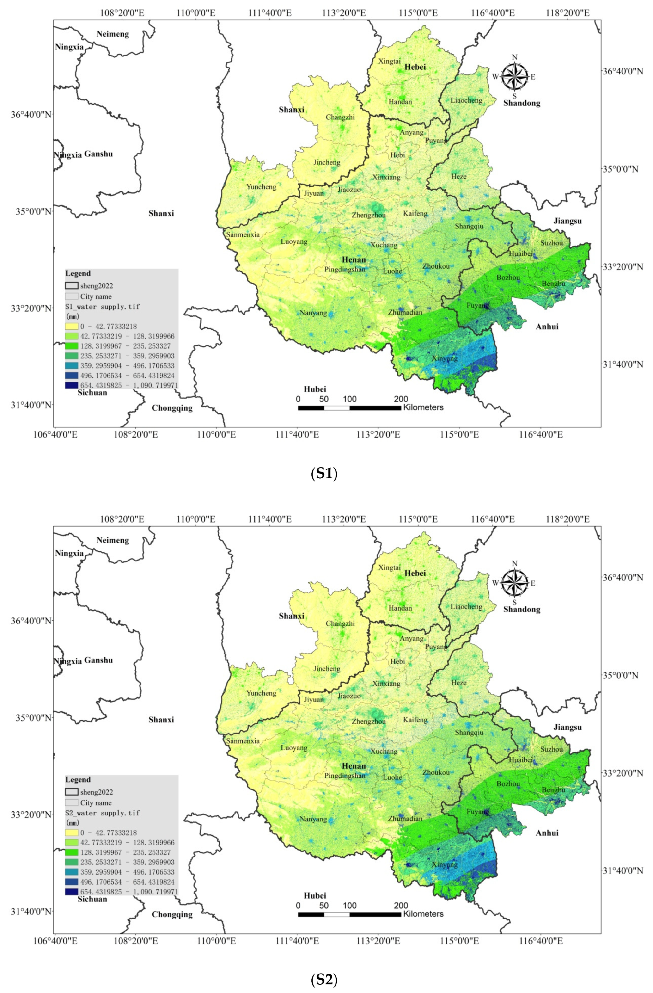
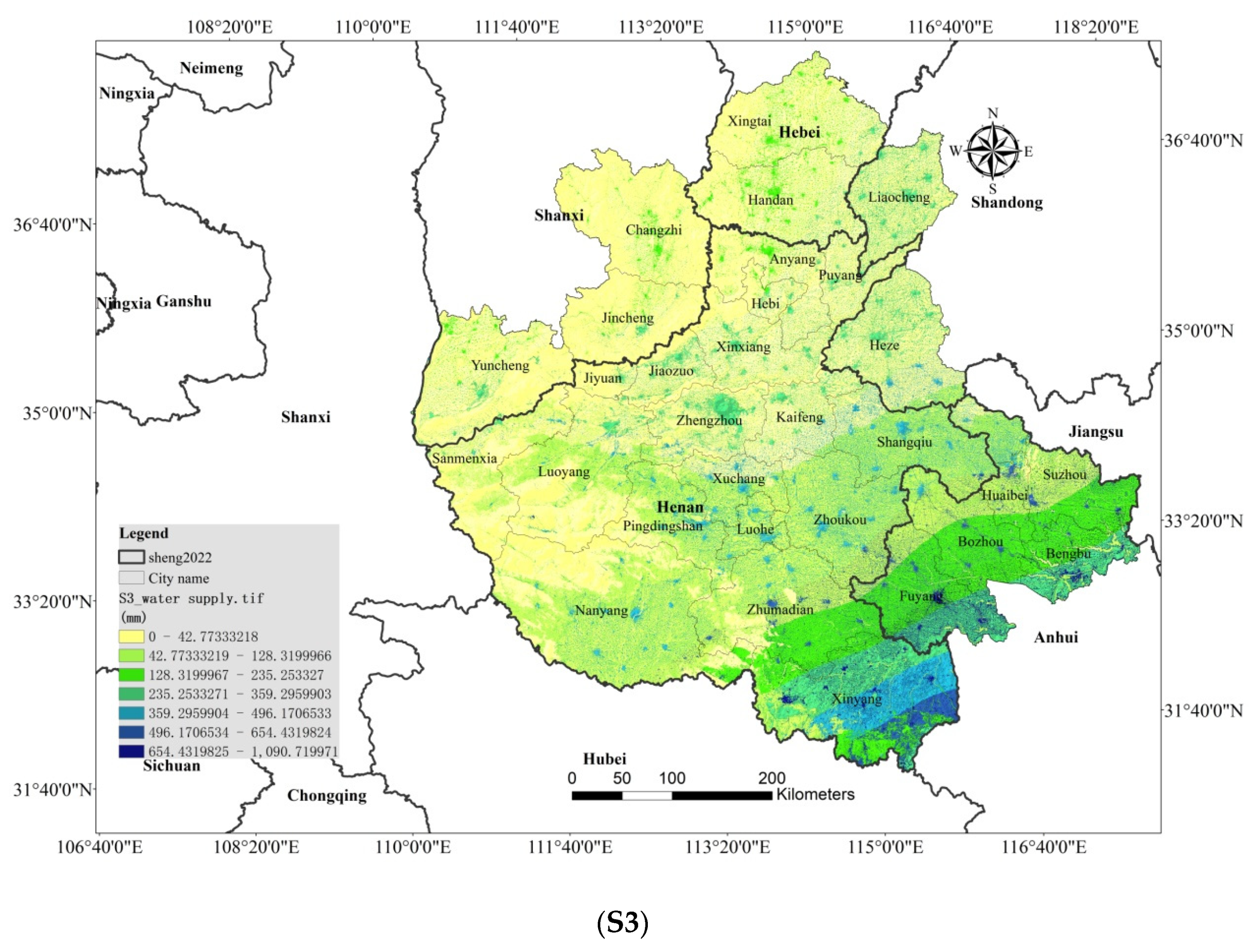
2.3.1. Water Supply Service

Water supply service refers to the amount of water available for human use in the study area:

$${\mathrm{Y}}_{\mathrm{x}\mathrm{j}}=(1-\frac{{\mathrm{A}\mathrm{E}\mathrm{T}}_{\mathrm{x}\mathrm{j}}}{{\mathrm{P}}_{\mathrm{x}}})\times {\mathrm{P}}_{\mathrm{x}}$$

(1)

where Y_xj is the annual water quantity of land cover type j in grid x in mm, AET_xj is the actual evapotranspiration of land cover type j in grid x in mm, and P_x is the precipitation in grid x in mm.

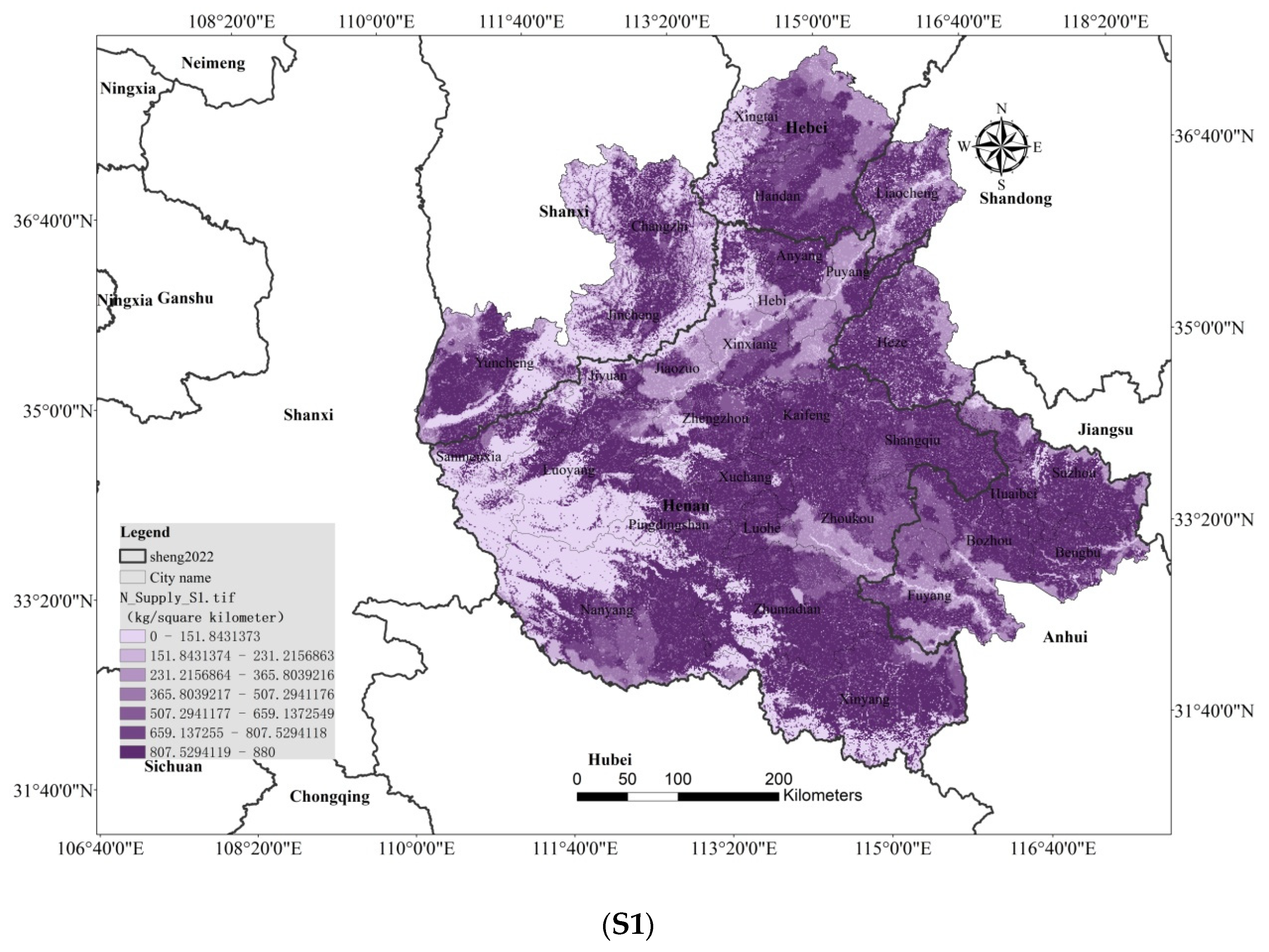
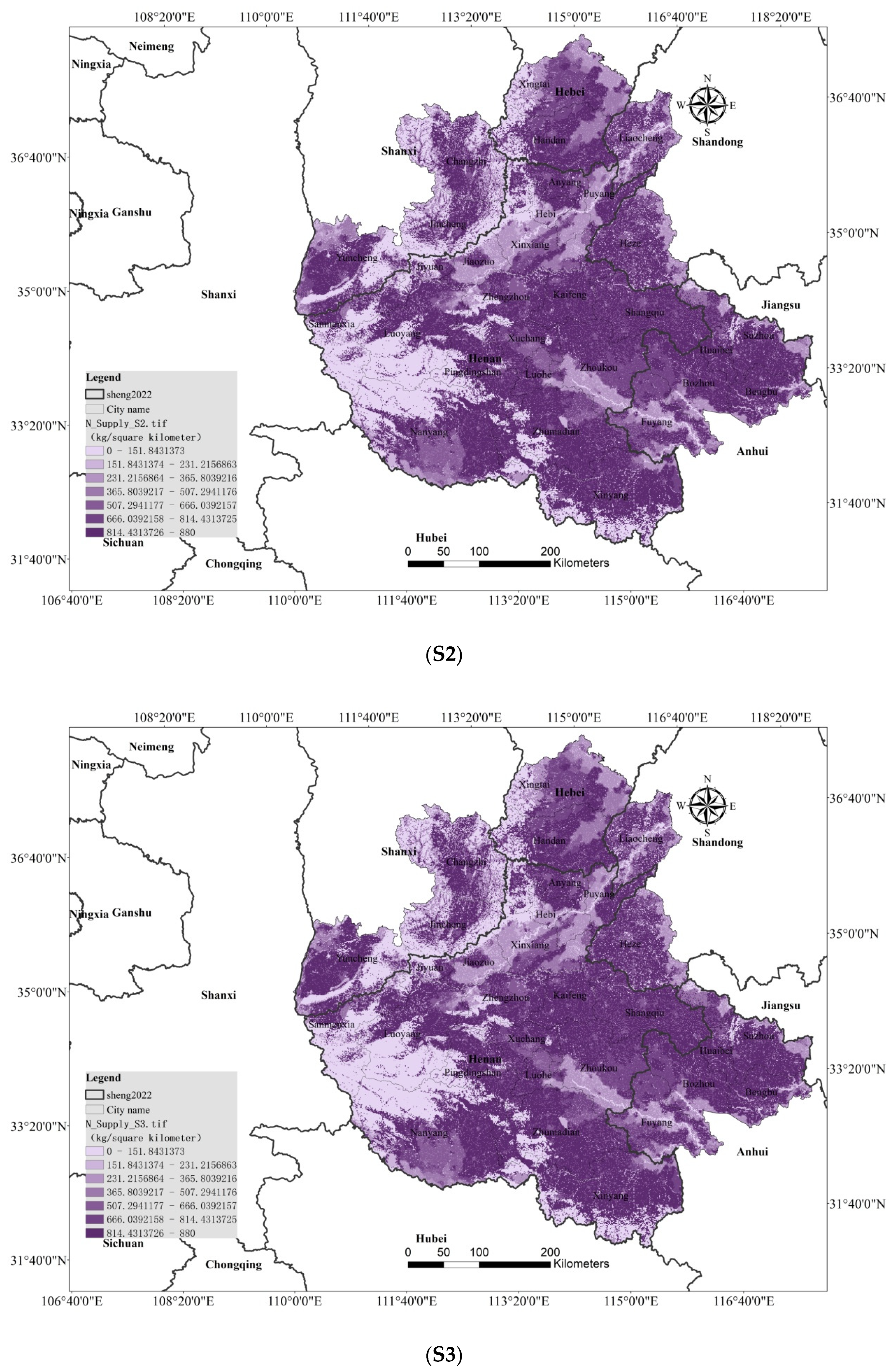
2.3.2. Water Purification (Nitrogen (N) Retention) Service

Water purification services refers to the ability of natural ecosystems to remove or reduce (purify) water pollutants, and the level of total nitrogen purification can reflect the level of water purification capacity of an ecosystem in a region:

$${\mathrm{A}\mathrm{L}\mathrm{V}}_{\mathrm{x}}={\mathrm{H}\mathrm{S}\mathrm{S}}_{\mathrm{x}}\times {\mathrm{p}\mathrm{o}\mathrm{l}}_{\mathrm{x}}$$

(2)

where ALV_x is the adjusted N output of grid x, HSS_x is the hydrological sensitivity score of grid x, and pol_x is the N output coefficient of grid x. After obtaining the N output, the purification amount is calculated according to the removal efficiency of N for each land use or land cover type.

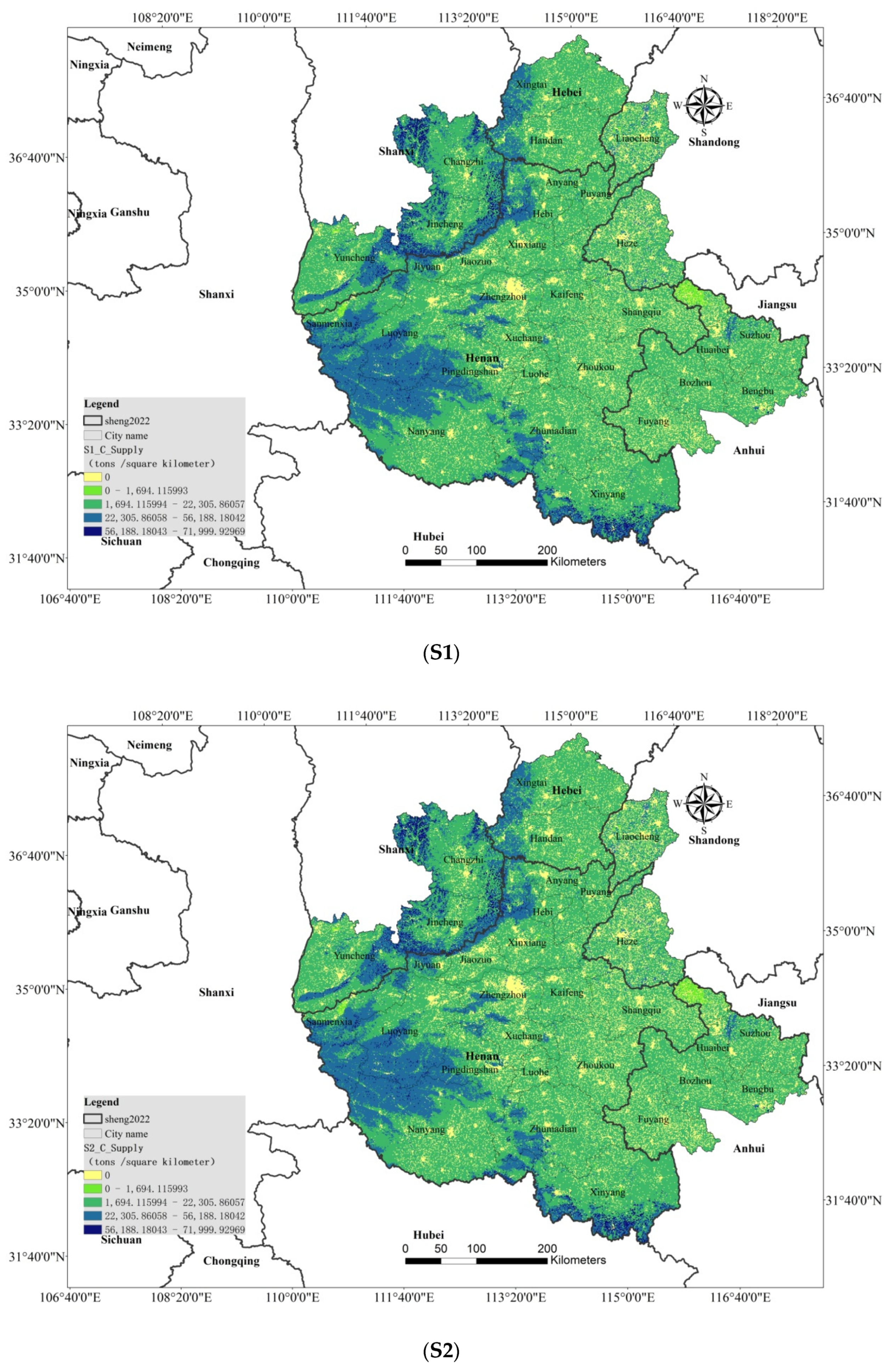
2.3.3. Carbon Service

Carbon service refers to the amount of carbon dioxide that can be absorbed by a “carbon sink” ecosystem in the study area.

$${\mathrm{C}}_{\mathrm{t}\mathrm{o}\mathrm{t}\mathrm{a}\mathrm{l}}={\mathrm{C}}_{\mathrm{b}\mathrm{e}\mathrm{l}\mathrm{o}\mathrm{w}}+{\mathrm{C}}_{\mathrm{a}\mathrm{b}\mathrm{o}\mathrm{v}\mathrm{e}}+{\mathrm{C}}_{\mathrm{s}\mathrm{o}\mathrm{i}\mathrm{l}}+{\mathrm{C}}_{\mathrm{d}\mathrm{e}\mathrm{a}\mathrm{d}}$$

(3)

where ${\mathrm{C}}_{\mathrm{t}\mathrm{o}\mathrm{t}\mathrm{a}\mathrm{l}}$ is the total carbon storage, C_bellow is the carbon storage of underground biomass, C_above is the carbon storage of the aboveground biomass, C_soil is the carbon storage of the soil carbon pool, and C_dead is the dead organic carbon storage.

The demand for carbon service is as follows:

$${\mathrm{C}}_{\mathrm{e}}={\sum }_{\mathrm{x}=1}^{\mathrm{X}}\mathrm{p}\left(\mathrm{x}\right)\times \mathsf{\phi }\left(\mathrm{x}\right)$$

(4)

where C_e is the carbon emissions from human social and economic activities (i.e., the carbon source), p(x) is the spatial population density of grid x, $\mathsf{\phi }\left(\mathrm{x}\right)$ is the carbon emissions per capita in grid x, and X is the total number of grids in the study area.

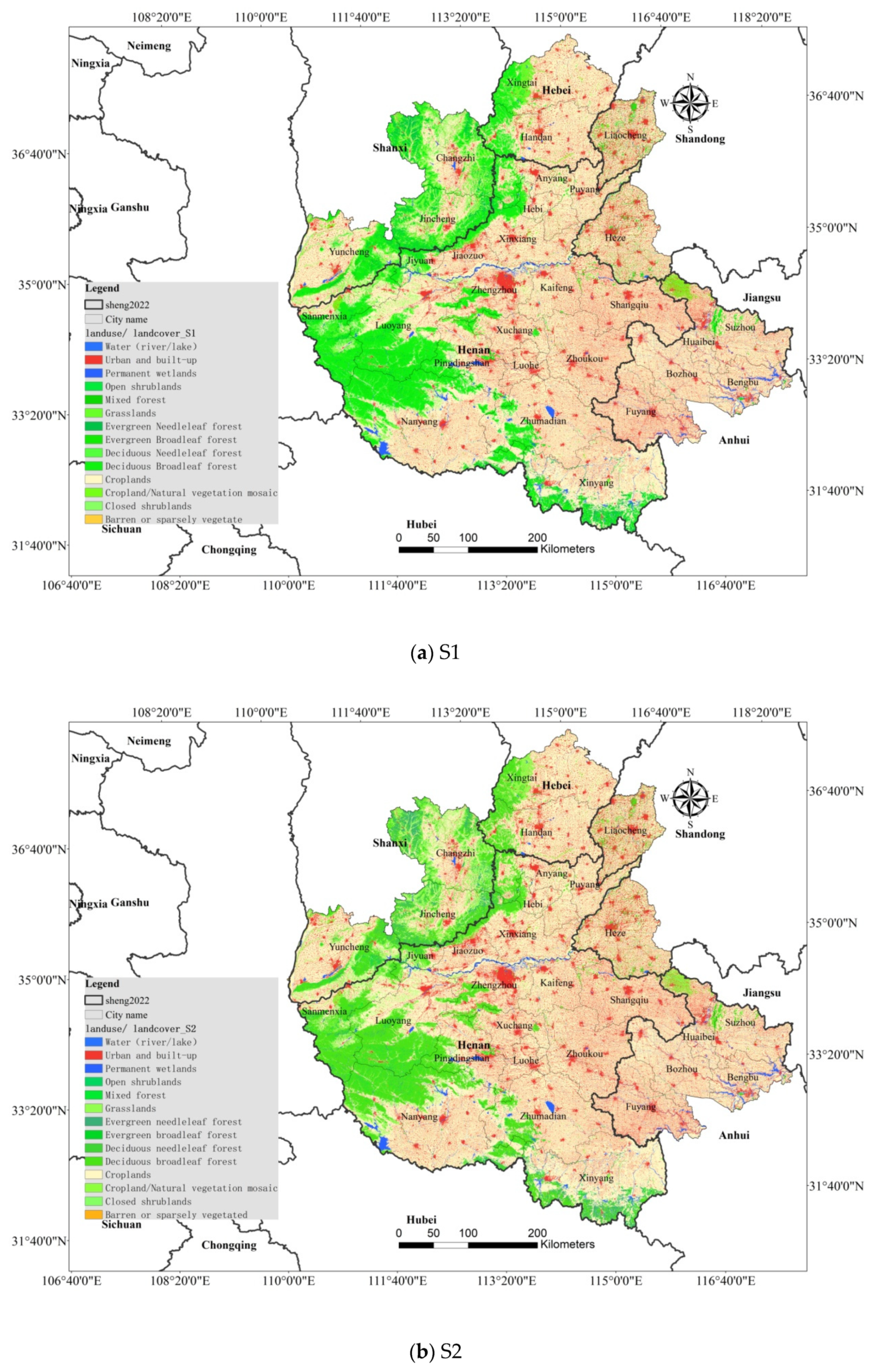
2.3.4. Scenario Analysis Setting

Based on the data for 2015, this study set three scenarios: planning, development, and protection. Under different scenarios, the land use/land cover (

Table 1. Land use/land cover (ecosystem types) of the CPUA.

Land Use/Land Cover	S1		S2		S3
	Area (km2)	Proportion (%)	Area (km2)	Proportion (%)	Area (km2)	Proportion (%)
Water (river/lake)	83	0.03	83	0.03	83	0.03
Evergreen needleleaf forest	5682	1.99	5682	1.99	5682	1.99
Evergreen broadleaf forest	2	0.00	2	0.00	2	0.00
Deciduous needleleaf forest	1	0.00	1	0.00	1	0.00
Deciduous broadleaf forest	43,621	15.26	43,621	15.26	43,621	15.26
Mixed forest	1430	0.50	1430	0.50	3379	1.18
Closed shrublands	50	0.02	46	0.02	50	0.02
Open shrublands	118	0.04	117	0.04	118	0.04
Grasslands	13,700	4.79	13,632	4.77	13,717	4.80
Permanent wetlands	5961	2.09	5916	2.07	5971	2.09
Croplands	172,289	60.27	170,664	59.70	170,801	59.75
Urban and built-up areas	41,226	14.42	42,980	15.03	40,739	14.25
Mixed cropland/natural vegetation areas	1390	0.49	1382	0.48	1389	0.49
Barren or sparsely vegetated areas	329	0.12	326	0.11	330	0.12

, Figure 2) is as follows:

Planning scenario (S1): To conduct urbanisation construction according to the “CPUA Development Plan 2016–2020”, the land for urban expansion is 33,821 ha, mainly from adjacent open shrublands, closed shrublands, grasslands, croplands, mixed cropland/natural vegetation areas, and barren or sparsely vegetated areas.

Development scenario (S2): According to the evolution trend from 2010 to 2020, urban and built-up areas rapidly expanded to the periphery with an increase of 209,237 ha. Urban expansion land mainly came from adjacent open shrublands, closed shrublands, grasslands, croplands, mixed cropland/natural vegetation areas, and barren or sparsely vegetated areas.

Protection scenario (S3): According to the target of the ecological space scale in 2010, permanent wetlands, including woodland, grassland, and wetland, will expand the ecological land, shrink the construction land and farmland, and implement the ecological protection strategy to increase grassland, woodland, and wetland by 194,855 ha.

2.3.5. Ecosystem Service Optimisation

This study used the Matlab software platform and the NSGA-II optimisation model to obtain a Pareto optimal solution set. The specific steps were as follows:

First, determine the initial solution. Based on the land use data at the end of 2015, this study evaluated water supply, water purification (N retention), and carbon sequestration ecosystem services in the study area under three scenarios as the initial solution to ecosystem service optimisation.

Second, the Pareto optimal solution set was obtained by running the optimisation model (NSGA-II) (

Table 2. Mathematical description of ecosystem service optimisation.

Algorithm	Objective Function	Decision Variable	Constraints
NSGA II	$\mathrm{Z}=\mathrm{M}\mathrm{a}\mathrm{x}\left\{{\mathrm{E}\mathrm{S}}_{\mathrm{I}}\left(\mathrm{X}\right),{\mathrm{E}\mathrm{S}}_{\mathrm{J}}\left(\mathrm{X}\right)\right\}$, where ESi and ESj represent a pair of ecosystem services with a trade-off or synergistic relationship.	The land use/land cover area and layout of various spatial elements.	(1) Structural constraints Area: ${\mathrm{X}}_1+{\mathrm{X}}_2+\cdots \dots +{\mathrm{X}}_{\mathrm{i}}=\mathrm{A}$ Structure: $\underset{{\mathrm{X}}_{\mathrm{i}}}{\to }$ (e.g., slope, topography, soil, and hydrology) Xi: the area of class i land use type in the region; A: the total area of the study area $\underset{{\mathrm{X}}_{\mathrm{i}}}{\to }$ (e.g., slope, topography, soil, and hydrology): the spatial distribution of class i land use types must meet the requirements of the slope, terrain, soil type, and hydrological conditions. (2) Service constraints: ${\mathrm{E}\mathrm{S}}_{\mathrm{i}}\ge {\mathrm{E}\mathrm{S}}_{\mathrm{m}\mathrm{i}\mathrm{n}}$ the class i ecosystem service; ${\mathrm{E}\mathrm{S}}_{\mathrm{m}\mathrm{i}\mathrm{n}}$: the minimum value required for the i-th ecosystem service.

). The optimisation constraints included structural and service constraints: Land area constraints: the cropland area was not less than 110 million mu (73,334 km²), and the eco-space area composed of water (river/lake), evergreen needleleaf forest, evergreen broadleaf forest, deciduous needleleaf forest, deciduous broadleaf forest, mixed forest, closed shrublands, open shrublands, grasslands, and permanent wetlands were not less than 16,835.70 km²; Land layout constraints: all land layout conditions consider factors such as slope, terrain, soil, and hydrology. Farmland with a slope >20 degrees should be returned to forest and grassland. To ensure the integrity of the ecological spatial structure, illegal industrial, mining, construction, and other lands should be relocated, and ecological land should be reserved in the river corridors of the southern Yellow River and the southern Huaihe River, as well as the ecological corridors of the Taihang Mountain, Funiu Mountain, and Liankang Mountain; Service constraints: considering the evaluation results of ecosystem service supply and demand in the study area and its natural socioeconomic characteristics, the study area’s water supply service should be ≥40 billion cubic metres, water purification (N retention) service should be ≥45,000 tons, and carbon service should be ≥1 billion tons to meet the ecosystem constraints.

Finally, the above optimal solutions were screened through expert consultation and other means, and the optimal solutions with practical application potential and corresponding land use structure schemes were retained, laying the foundation for optimising the land use structure of ecological space in the next step.

2.3.6. Methods of Land Use/Land Cover Optimisation and Adjustment

First, the pre-optimisation land cover/use map (i.e., current land cover/use map) and the optimised land cover/use map were compared, and the area attributes and spatial positions of different land cover/use types were extracted. The combined conversion requirements for land cover/use between them were calculated. Then, the expert knowledge method was adopted to select the suitable land use combination and form the ecological spatial structure optimisation scheme. Considering the influence of the international situation on food security in the present and future, this study, combined with the function positioning of the central region as a grain production area, determined the farmland protection priority, ecological land protection as far as possible, the development of construction land stock, the minimum increase for construction land and other principles, and established the optimal layout of land use types.

In specific operations, we optimised the conversion of the land cover type according to the principles of preferential conversion of land type similarity, preferential conversion of the close distance, and preferential conversion of land type with low difficulty. The conversion process and results mainly used the InVEST model Scenario Generator module. The spatial layout was conducted through outward expansion from the target land class. The deciduous broadleaf forest optimisation adjustment order was deciduous needleleaf forest, evergreen broadleaf forest, and evergreen needleleaf forest. The croplands optimisation adjustment order was water, evergreen needleleaf forest, mixed forest, closed shrublands, open shrublands, grasslands and permanent wetlands, and mixed cropland/natural vegetation. The urban and built-up optimisation adjusted the order to mixed cropland/natural vegetation.

3. Results

3.1. Initial Value of the Current Supply and Demand Situation of Ecosystem Services

The analysis showed that the total annual supply of the water supply service was less than the total freshwater demand under the three scenarios. The total supply of the water purification (N retention) service was smaller than its total demand. The total supply of the carbon service was greater than its total demand (

Table 3. Ecosystem service supply under different scenarios before optimisation.

	ES1: Water Supply Service (108 Cubic Metres)	ES2: Water Purification Service (104 tons)	ES3: Carbon Service (108 tons)
S1	336.00	5.76	29.40
S2	341.00	5.72	29.40
S3	334.00	5.74	30.40

and

Table 4. Ecosystem service demand under different scenarios before optimisation.

	ES1: Water Supply Service (108 Cubic Metres)	ES2: Water Purification Service (104 tons)	ES3: Carbon Service (108 tons)
S1	527.62	11.4	10.72
S2	535.73	11.4	10.00
S3	523.30	11.4	10.04

). In terms of supply, S1 had 33.60 billion cubic metres of water supply, 57,600 tons of water purification (N retention), and 2.94 billion tons of carbon sequestration; S2 had 34.10 billion cubic metres of water supply, 57,200 tons of water purification (N retention), and 2.94 billion tons of carbon sequestration; S3 had 33.40 billion cubic metres of water supply, 57,400 tons of water purification (N retention), and 3.04 billion tons of carbon sequestration. In terms of demand, the water supply service demand in different scenarios was 52.762 (S1), 53.573 (S2), and 52.330 (S3) billion cubic metres; the water purification (N retention) service demand was 114,100 tons; while the carbon service demand was 1.072, 1.000, and 1.004 million tons, respectively.

Regarding spatial distribution (Figure 3, Figure 4 and Figure 5), the water supply service has a pattern of less in the north and more in the south, and the water supply service per unit area of land gradually increased from north to south. Carbon service areas are mainly located in the Taihang and Funiu Mountains in the west and the Liankang Mountains in the south. The water purification (N retention) service had a pattern of high peripheral and low central farmland.

Since the study area is the location of the middle route of the South-to-North Water Diversion project, the water supply service of the CPUA has additional resources, and the future water supply service output of the local natural ecosystem of ≥40 billion cubic metres can meet the demand. Since the nitrogen emissions of CPUA (using the main province of Henan as an example) have exceeded the nitrogen water environmental capacity of the study area, urban and rural sewage treatment projects in the study area have been included in the national and local government work plan. The future water purification (N retention) service output of the local natural ecosystem of ≥45,000 tons can meet the demand. The total supply of carbon service is greater than its total demand, which can be met by keeping the carbon service up to 1 billion tons.

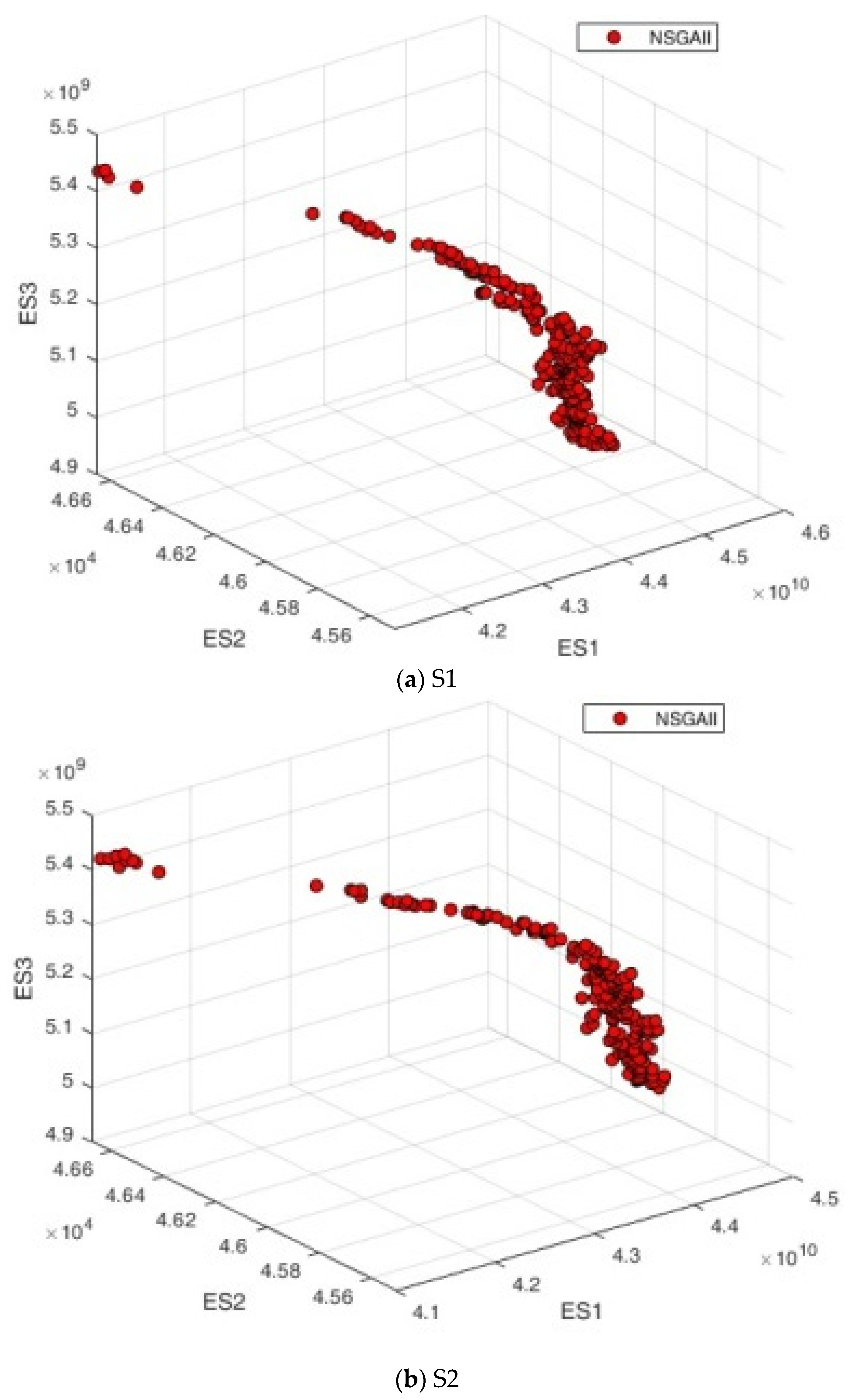
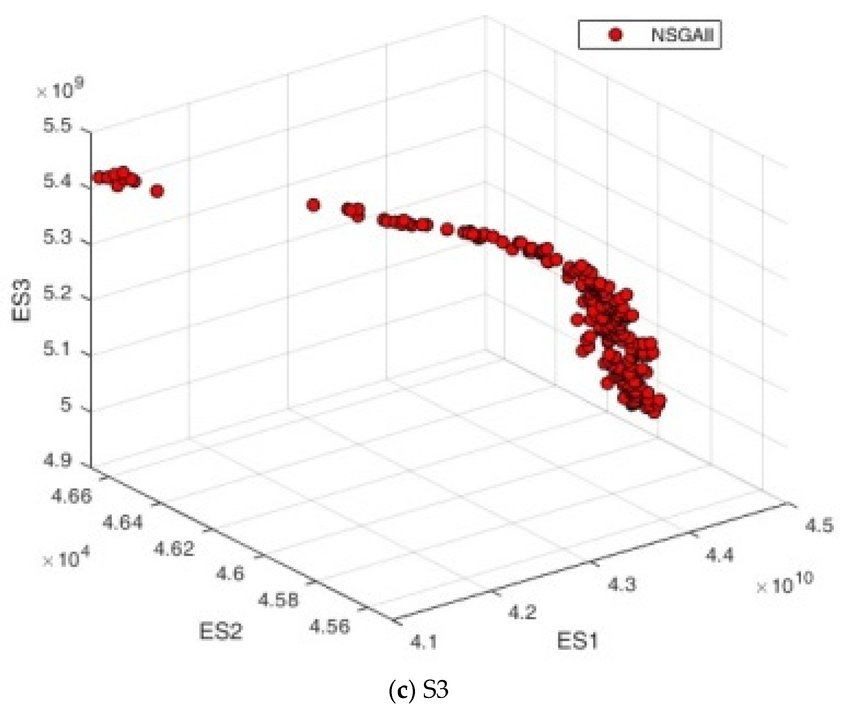
3.2. The Pareto Optimal Solution for Ecosystem Services

In the Matlab platform, the NSGA-II optimisation model was used to obtain water supply (ES1), water purification (N retention) (ES2), and carbon storage and sequestration (ES3) under different scenarios to determine the three-objective Pareto optimal solution set between services. The results showed 199, 197, and 197 optimal solutions for the water supply (ES1), water purification (N retention; ES2), and carbon storage and sequestration (ES3) services under S1, S2, and S3, respectively (Figure 6). Based on the Pareto curve’s optimal solution screening method, combined with the urgency of different ecosystem services in the study area, the potential of alternative resources of ecosystem services, and the surplus/shortage of total ecosystem services, we determined the three-objective Pareto optimal solution between water supply, water purification (N retention), and carbon service under S1 (442.82, 4.62, and 54.27, respectively), S2 (423.43, 4.62, and 54.06, respectively), and S3 (412.32, 4.66, and 54.20, respectively).

Under this optimisation goal, to achieve Pareto optimality of ecosystem services, the water supply, water purification (N retention), and carbon service must be optimised simultaneously, and ecosystem services must be optimised and adjusted. Under S1, the water supply service needs to increase by 10.682 billion cubic metres, the water purification (N retention) service needs to decrease by 11,400 tons, and the carbon service needs to decrease by 2.487billion tons. Under S2, the water supply service needs to increase by 8.243 billion cubic metres, the water purification (N retention) service needs to decrease by 11,000 tons, and the carbon service needs to decrease by 2.466 billion tons. Under S3, the water supply service needs to increase by 4.089 billion cubic metres, the water purification (N retention) service needs to decrease by 10,800 tons, and the carbon service needs to decrease by 2.380 billion tons.

3.3. Land Use Optimisation Based on Ecosystem Services

3.3.1. Land Use Area Optimisation

In this study, the land use/land cover in the study area was assumed to be a single type. The ecosystem service quantity of a single land use type in the study area was obtained using the InVEST model and the corresponding model’s input coefficient, which was the conversion coefficient between land use types to provide data relations for land optimisation and adjustment based on ecosystem service. Among the results (

Table 5. Ecosystem services of land use/land cover per unit area.

Land Use/Land Cover	Water Supply Service (108 cubic metre/km2)	Water Purification (N Retention) Service (104 tons/km2)	Carbon Service (108 tons/km2)
Water	491.3	0.005	0
Evergreen needleleaf forest	51.3	135	72,000
Evergreen broadleaf forest	51.3	144	52,500
Deciduous needleleaf forest	51.3	144	56,400
Deciduous broadleaf forest	51.3	144	47,500
Mixed forest	51.3	144	52,500
Closed shrublands	158.24	100	29,000
Open shrublands	51.3	144	22,500
Grasslands	102.55	160	3400
Permanent wetlands	51.3	160	4000
Croplands	120.69	275	1800
Urban and built-up areas	412.51	36.25	0
Mixed cropland/natural vegetation areas	102.55	132.5	1400
Barren or sparsely vegetated areas	412.51	20	0

), the largest land use type of the water supply service was water, and the conversion coefficient for this ecosystem service was 49.13 billion cubic metres/km². The highest conversion coefficient for the water purification (N retention) service was 2.75 million tons/km² for croplands. The smallest carbon service was for water, urban and built-up, and barren or sparsely vegetated areas with zero carbon service.

Based on the land use conversion coefficient, this study used the Matlab software platform and NSGA-II optimisation model to obtain the land use type area corresponding to the Pareto optimal solution for ecosystem services under different scenarios. To achieve the objective of ecosystem service optimisation in the study area (

Table 6. Land cover/land use Pareto optimal area under different scenarios.

Land Use/Land Cover	S1		S2		S3
	Area (km2)	Proportion (%)	Area (km2)	Proportion (%)	Area (km2)	Proportion (%)
Water	15,385	5.38	15,335	5.36	15,473	5.41
Evergreen needleleaf forest	15,415	5.39	15,446	5.40	15,471	5.41
Evergreen broadleaf forest	15,579	5.44	15,432	5.40	15,351	5.37
Deciduous needleleaf forest	15,288	5.34	15,382	5.38	15,524	5.43
Deciduous broadleaf forest	15,434	5.39	15,393	5.38	15,447	5.40
Mixed forest	15,648	5.47	15,440	5.40	15,532	5.43
Closed shrublands	15,497	5.42	15,351	5.37	15,239	5.33
Open shrublands	15,403	5.38	15,211	5.32	15,150	5.30
Grasslands	15,234	5.32	15,291	5.35	15,417	5.39
Permanent wetlands	14,956	5.23	14,811	5.18	15,250	5.33
Croplands	87,370	30.54	87,904	30.75	87,680	30.67
Urban and built-up areas	14,075	4.92	14,056	4.92	15,495	5.42
Mixed cropland/natural vegetation	12,544	4.38	12,300	4.30	15,385	5.38
Barren or sparsely vegetated areas	18,291	6.39	18,540	6.48	13,478	4.71

), deciduous broadleaf forests, croplands, and urban and built-up areas were the diversion sides in land conversion (Figure 7). Under S1, deciduous broadleaf forests, croplands, and urban and built-up areas must transfer 28,187, 84,919, and 27,151 km², respectively. Under S2, deciduous broadleaf forests, croplands, and urban and built-up areas must transfer 28,228, 82,760, and 28,924 km², respectively. Under S3, deciduous broadleaf forests, croplands, and urban and built-up areas require 28,174, 83,121, and 25,244 km², respectively.

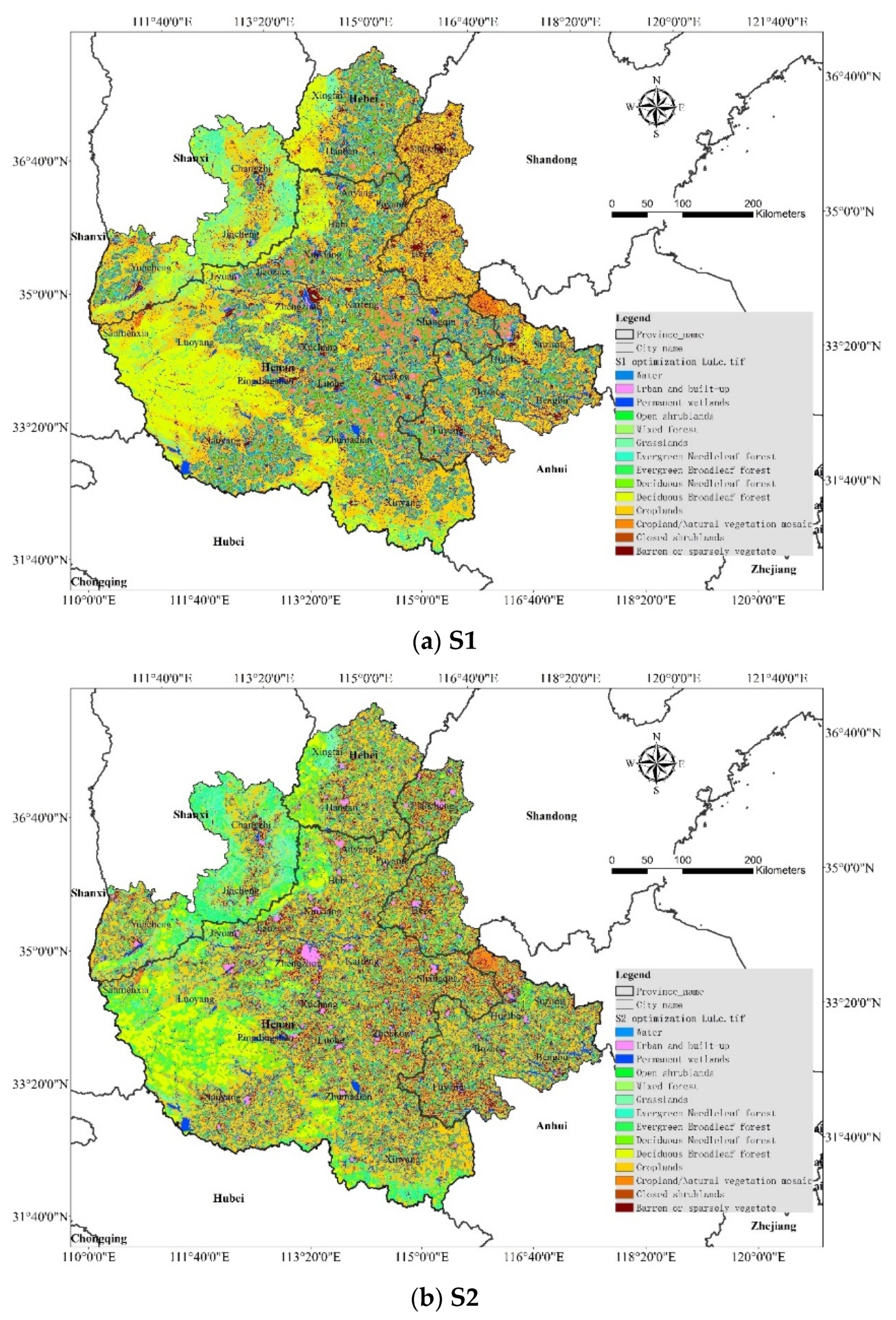
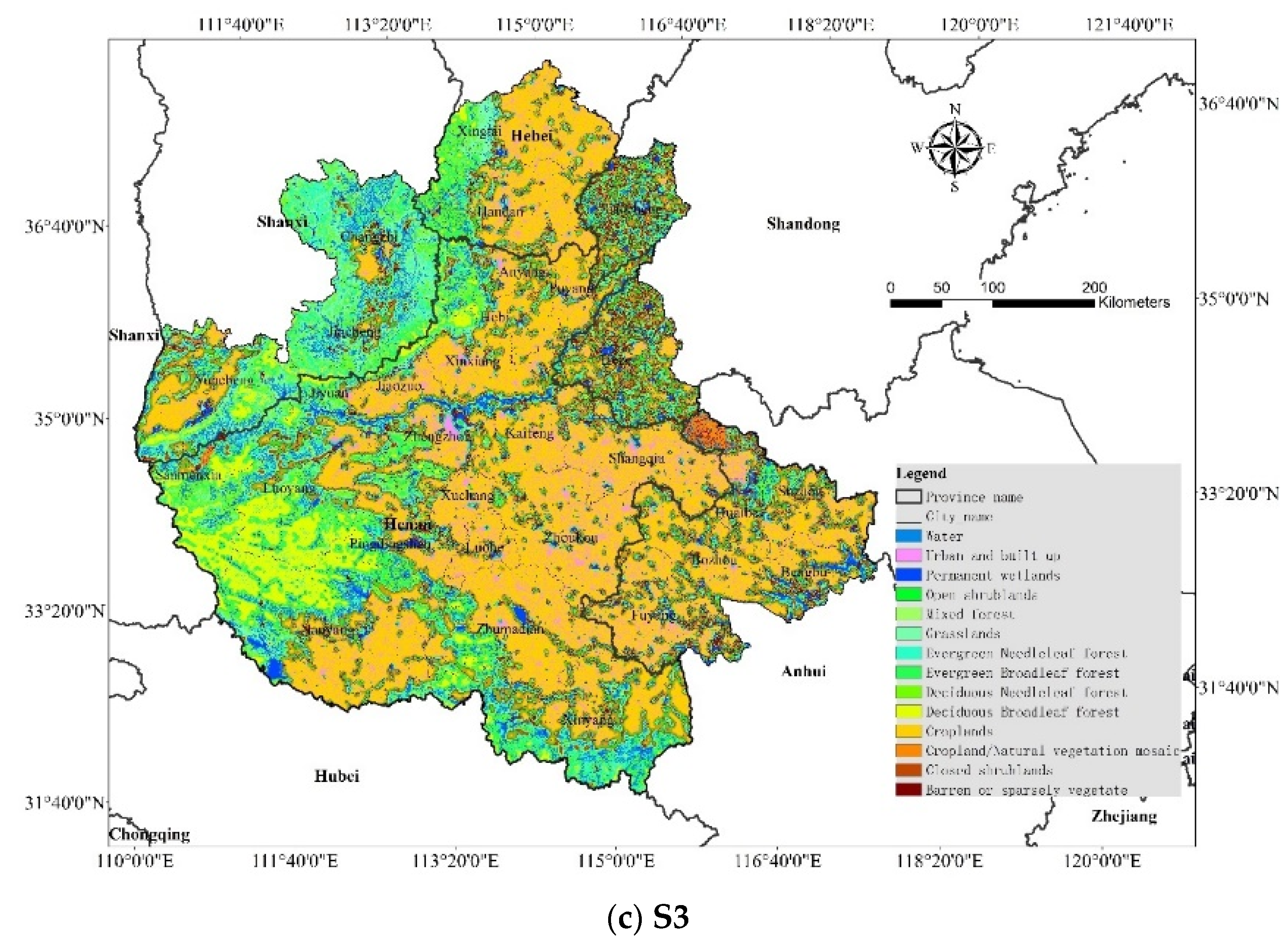
3.3.2. Scenario Optimisation Selection Based on Land Use Pattern

As shown in Table 6, to achieve the goal of ecosystem service optimisation in the study area, the deciduous broadleaf forest in the mountainous area, the croplands in the central area, and the urban and built-up areas all decreased in different scenarios. In contrast, water, evergreen needleleaf forests, evergreen broadleaf forests, deciduous needleleaf forests, mixed forests, closed shrublands, open shrublands, grasslands, permanent wetlands, mixed cropland/natural vegetation, and barren or sparsely vegetated areas were the primary land importers and increased in area accordingly. The optimised land cover/land use structure under different scenarios is shown in Figure 8: The central and eastern regions were mainly cropland and urban and built-up areas. The mountains to the west and south were mainly evergreen needleleaf forests, evergreen broadleaf forests, deciduous needleleaf forests, mixed forests, closed shrublands, open shrublands, and grasslands.

Regarding the optimised planning (S1; 33,821 ha) and development (S2; 209,237 ha) scenarios, open shrublands, closed shrublands, grasslands, croplands, and mixed cropland/natural vegetation adjacent to urban and built-up and barren or sparsely vegetated areas were mainly converted into urban and built-up areas (S1: 33,821 ha; S2: 209,237 ha), leading to severe fragmentation of land use structure in the middle of S1 and S2 after optimisation, damaging the integrity of the ecosystem in the central region, which may affect ecosystem service processes and functions and reduce the sustainable supply capacity of ecosystem services. In the optimised conservation scenario (S3), water, evergreen needleleaf forests, evergreen broadleaf forests, deciduous needleleaf forests, mixed forests, closed shrublands, open shrublands, grasslands, and permanent wetlands adjacent to 194,855 ha of croplands and urban and built-up areas were converted into evergreen needleleaf forest, evergreen broadleaf forest, deciduous needleleaf forest, mixed forest, closed shrubland, open shrubland, grassland, or permanent wetland. After land use optimisation and adjustment, the ecological land structure of S3 was complete; the ridgelines of Taihang Mountain, Funiu Mountain, and Liankang Mountain in the north, west, and south were more continuous; the river corridor structures of the Yellow River and Huaihe River were more complete; and the croplands in the middle were distributed in concentrated contiguous areas. The land use structure was more consistent with the study area’s ecological protection and urban development vision. Therefore, S3 was selected as the optimal scenario in this study.

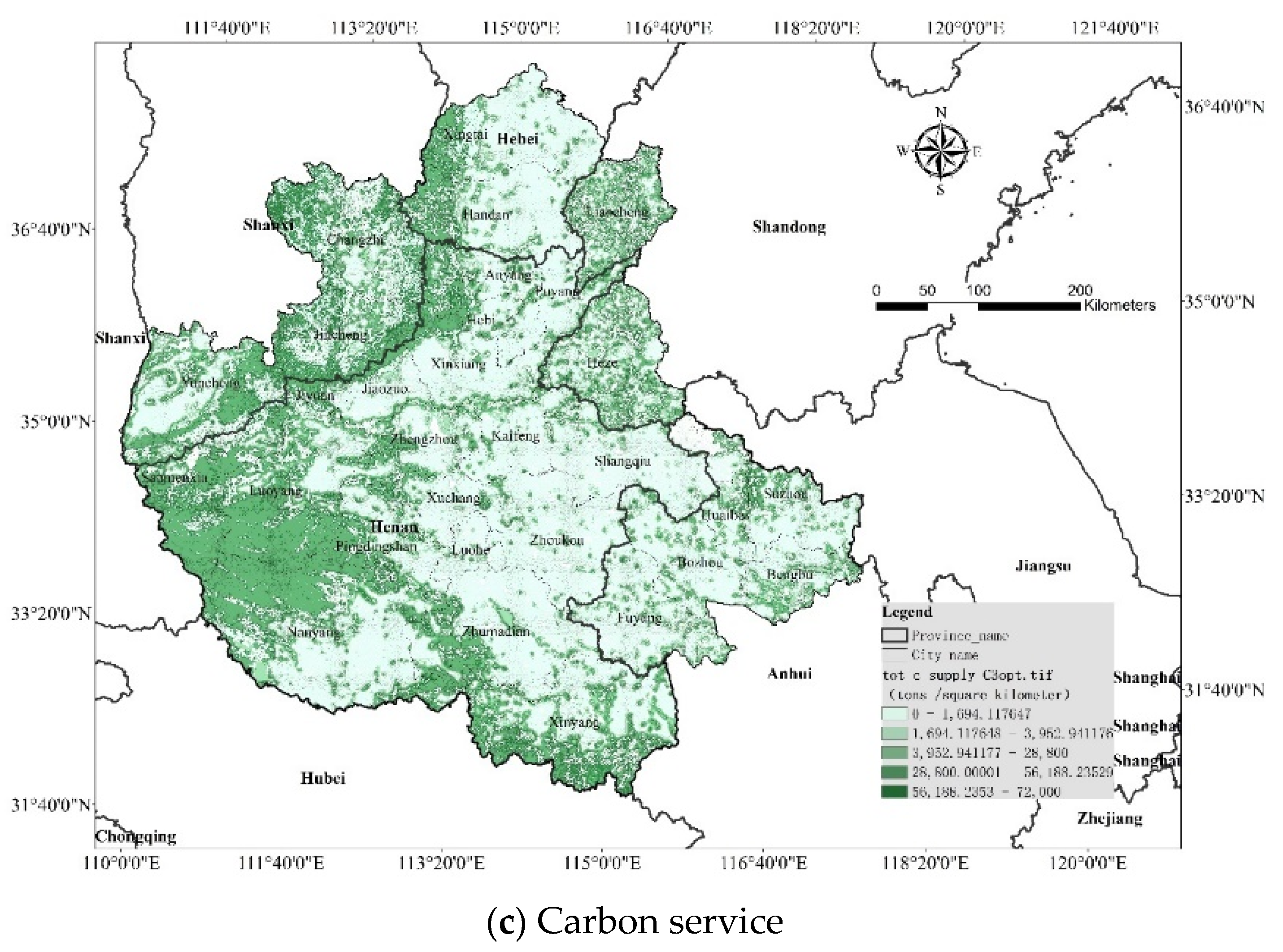
3.4. Optimisation of the Supply Pattern of Ecosystem Services

The optimised S3 is the optimal scenario in this study. Based on the optimised S3 land use/landcover pattern, this study quantified the ecosystem service supply pattern in the study area and obtained its optimisation results. The results show (Figure 9) that, after optimisation, the water supply service increased in the central and western parts of the study area, improving the potential of farmland production activities and urban water supply in populated areas in the central part of the study area. After optimisation, the demand zone (negative zone) of the water purification (N retention) service in the central area was reduced, the supply zone of the water purification (N retention) service was connected to the study area and had better connectivity, and the supply and demand zones were more closely combined. After optimisation, the carbon service supply in the central part of China increased, connecting the eastern and western ecosystem service supply areas. The carbon service’s supply pattern in the study area was more balanced after optimisation.

4. Discussion

Human society depends on ecosystem services to survive, and humans are the primary users of ecosystem services. Only when the supply of ecosystem services matches people’s demand can the management of ecosystem services play a large role [1]. Optimising ecosystem service based on demand is the core content of ecosystem service management [10]. Pareto frontiers have been widely used in determining the objectives of ecosystem service optimisation [14]. The Pareto curve of ecosystem services (Pareto frontiers) is mathematically represented as a curve in an axis. Each point in the curve (Pareto frontier) represents an optimal combination of solutions, meaning that, when an ecosystem service remains in the same constant state, the maximum possible value of other ecosystem services (the area under the curve) is suboptimal; that is, when the solution ES is in the same constant state under this solution set, other ecosystem services still have room for improvement by adjusting the spatial land pattern. In selecting the optimal implementation path, regional land use change can significantly change the pattern and process of the ecosystem, leading to a change in ecosystem service supply [2,34,35]. Therefore, many scholars believe that the optimisation realisation approach is mainly to optimise the land use under the guidance of ecosystem services and seek the potential of improving the supply of ecosystem services by determining the optimal land use pattern under a certain optimal ecosystem service (Figure 10) [34,36,37]. The optimisation of ecosystem services and the optimisation and adjustment of land use patterns based on it also have clear spatial guidance for optimising the land use planning scheme in the study area [38]. Based on this, the optimisation of ecosystem services is often used to guide the formulation of regional land planning and natural resource management policies [13,39,40,41].

Currently, focusing on the supply potential and demand of ecosystem services, some studies have explored how to optimise the supply pattern of ecosystem services and match their demand through land pattern optimisation. Some researchers believe land management based on ecosystem services combines environmental characteristics and social needs. Coupling ecosystem service supply and demand with landscape ecological security patterns is the basis for optimising regional ecological spatial layout [11,16,17,42]. It also provides important opportunities and options for achieving global sustainable development goals [34,43]. Yue et al. took Guyuan City in the Ningxia region as an example. Based on multi-source data, they used the InVEST model, coupled coordination degree model, spatial autocorrelation, and other methods to quantise the supply and demand of regional ecosystem services by taking the township as the scale unit, building the matching and coordination relationship between supply and demand, and designating the ecological restoration zones according to the natural resources and social and economic development characteristics within the zones. They proposed corresponding optimisation strategies to provide scientific support for local managers to conduct ecological restoration practices [44].

Rong et al. identified the source and node of ecosystem service supply and demand in the Xiongan New Area from the supply and demand of ecosystem services, constructed the ecological network of the new area, optimised the regional ecosystem service supply pattern, and explored the optimisation method of urban ecological pattern to improve the regional ecosystem service supply capacity and match the ecosystem service demand [45]. Taking Kunshan City in Jiangsu Province as an example, Wang and Wang analysed the spatial demands of four ecosystem services: rain-flood regulation, habitat protection, leisure and recreation, and culture and entertainment. Based on the principle of matching supply and demand, they planned a waterfront greenway by sections and types and proposed spatial development guidelines, providing new ideas for the planning and construction of waterfront greenways [46].

Regarding methods, the supply and demand of ecosystem services are often evaluated using biophysical models, such as the InVEST model. Due to the fact that the InVEST model can reflect the dynamic process and spatial change in ecosystem services caused by land use change, it is widely used in evaluating the impact of land use on various ecosystem services [39,47,48]. However, due to the lack of basic data, the reliability and accuracy of the evaluation results obtained using InVEST model need to be improved [49]. For example, in a quantitative evaluation study of water production, the temporal and spatial distribution characteristics of annual water production were closely related to the accuracy of the average annual temperature, actual annual evapotranspiration, and rainfall data in the study area [50]. The accuracy of land use and vegetation type distribution data has an important impact on the accuracy of the evaluation results for the spatiotemporal pattern of carbon storage in the study area [51]. The evaluation of ecosystem and water purification services is greatly restricted by the accuracy of terrain, soil, and other spatial data [52].

In urban agglomerations, soil, hydrology, vegetation, water quality, and other parameters are greatly affected by human activities [49,53] and differ significantly from the natural state. There are currently few studies on ecosystem service evaluation in this region, and basic data are lacking [32,39,48,54,55]. Therefore, it is necessary to obtain relevant basic data through field observation and investigation combined with the actual situation of the study area, input these basic data into the model, and optimise the model parameters to more accurately simulate the supply potential of ecosystem services in urban agglomeration areas.

In addition, the distribution of Pareto optimal solution sets among the three services under different scenarios is not balanced, and partial solutions have a large deviation from the trend of the fitting curve, which may lead to inappropriate solutions. Therefore, screening the optimal solutions based on expert advice is necessary. Regarding the optimisation of ecosystem services, the mathematical model has a unique advantage in the output of the quantitative optimisation results of their supply scale. However, the spatial layout of the optimal scale of output ecosystem services needs to be combined with other models. In this study, we used the InVEST model scenario generator module to determine the spatial layout of the optimised land type scale and then used the InVEST model to present the optimised ecosystem service supply pattern. In this process, the selection of land use layout also needs to be guided by expert knowledge, so the professional background of experts is required to be relatively high. The possible disadvantage is that subjective factors, such as the professional level and authority of experts, the psychological state of experts, and the guidance of researchers to experts, may affect the accuracy of the land layout results. Further development of the optimisation model is needed to enable it to have strong spatial optimisation capability.

5. Conclusions

The supply and demand carbon service quantity and spatial pattern of water supply service, water purification (N retention) service, and carbon service in the CPUA were optimised, and the basic conclusions were as follows:

(1) Before optimisation, S1 could supply 33.66 billion cubic metres of freshwater, 57,600 tons of purified water (N retention), and 2.94 billion tons of carbon service; S2 could supply 34.10 billion cubic metres of freshwater, 57,200 tons of purified water (N retention), and 2.94 billion tons of carbon service; and S3 could supply 33.400 billion cubic metres of freshwater, 57,400 tons of purified water (N retention), and 3.04 billion tons of carbon service. The water supply service had a spatial pattern of less in the north and more in the south, the carbon service had a pattern of more in the west and less in the south, and the water purification (N retention) service had a pattern of high values in the periphery and low values in the central farmland area.

(2) The Pareto optimal solution for the water supply, water purification (N retention), and carbon service was 44.282 billion cubic meters, 46,200 tons, and 5.427 billion tons under S1; 42.343 billion cubic meters, 46,200 tons, and 5.406 billion tons under S2; 41.232 billion cubic meters, 46,600 tons, and 5.420 billion tons under S3.

(3) To achieve the Pareto optimal supply, the deciduous broadleaf forests in the mountain area, the croplands in the central area, and the urban and built-up areas all decreased to varying degrees under different scenarios. Water, evergreen needleleaf forests, evergreen broadleaf forests, deciduous needleleaf forests, mixed forests, closed shrublands, open shrublands, grasslands, permanent wetlands, mixed cropland/natural vegetation areas, and barren or sparsely vegetated areas were the main land use/land cover type that increased the areas. After land use optimisation and adjustment, the S3 was selected as the optimal scenario for its complete ecospace structure and concentrated contiguous croplands in the middle CPUA, which is consistent with the CPUA’s ecosystem protection and urban development vision. The optimised supply pattern of the water supply, water purification (N retention), and carbon service in the central CPUA greatly improved, which could connect ecosystem service supply areas in the western with ecosystem service supply areas in the eastern region and balance the overall ecosystem service supply pattern in the CPUA, and eventually improve the supply potential of the three ecosystem services and meet the demands. It is found that, from the perspective of ecosystem service supply and demand, the nonlinear relationship between urban agglomeration ecosystem services management and land use planning can be better understood, and spatial guidance can be provided for inter-city land use planning and ecosystem management policy formulation.

References

1. Ma, L.; Liu, H.; Peng, J.; WU, J. A review of ecosystem services supply and demand. Acta Geogr. Sin. 2017, 72, 1277–1289. [Google Scholar] [CrossRef]
2. Reid, W.V.; Mooney, H.A.; Cropper, A.; Capistrano, D.; Carpenter, S.R.; Chopra, K.; Dasgupta, P.; Dietz, T.; Duraiappah, A.K.; Kasperson, R.; et al. Millennium Ecosystem Assessment Synthesis Report. 2005. Available online: http://pdf.wri.org/mea_synthesis_030105.pdf (accessed on 20 June 2023).
3. López-Hoffman, L.; Varady, R.G.; Flessa, K.W.; Balvanera, P. Ecosystem services across borders: A framework for transboundary conservation policy. Front. Ecol. Environ. 2010, 8, 84–91. [Google Scholar] [CrossRef] [Green Version]
4. Shen, J.; Li, S.-C.; Liang, Z.; Wang, Y.; Sun, F. Research progress and prospect for the relationships between ecosystem services supplies and demands. J. Nat. Resour. 2021, 36, 1909–1922. [Google Scholar] [CrossRef]
5. Costanza, R. Ecosystem services: Multiple classification systems are needed. Biol. Conserv. 2008, 141, 350–352. [Google Scholar] [CrossRef]
6. Daily, G.C. Nature’s Services: Societal Dependence on Natural Ecosystems; Daily, G.C., Ed.; Island Press: Washington, DC, USA, 1997. [Google Scholar]
7. Cimon-Morin, J.; Darveau, M.; Poulin, M. Towards systematic conservation planning adapted to the local flow of ecosystem services. Glob. Ecol. Conserv. 2014, 2, 11–23. [Google Scholar] [CrossRef] [Green Version]
8. Bennett, E.M.; Peterson, G.D.; Gordon, L.J. Understanding relationships among multiple ecosystem services. Ecol. Lett. 2009, 12, 1394–1404. [Google Scholar] [CrossRef] [PubMed]
9. Kleemann, J.; Schrter, M.; Bagstad, K.J.; Kuhlicke, C.; Bonn, A. Quantifying interregional flows of multiple ecosystem services—A case study for Germany. Glob. Environ. Chang. 2020, 61, 102051. [Google Scholar] [CrossRef]
10. Xu, H.; Brown, D.G.; Moore, M.R.; Currie, W.S. Optimizing Spatial Land Management to Balance Water Quality and Economic Returns in a Lake Erie Watershed. Ecol. Econ. 2018, 145, 104–114. [Google Scholar] [CrossRef]
11. Hu, Q.; Chen, S. Optimizing the ecological networks based on the supply and demand of ecosystem services in Xiamen-Zhangzhou-Quanzhou region. J. Nat. Resour. 2021, 36, 342–355. [Google Scholar] [CrossRef]
12. Chen, J.; Jiang, B.; Bai, Y.; Xu, X.; Alatalo, J.M. Quantifying ecosystem services supply and demand shortfalls and mismatches for management optimisation. Sci. Total Environ. 2019, 650, 1426–1439. [Google Scholar] [CrossRef] [PubMed]
13. Yu, Y.; Li, J.; Zhou, Z.; Tang, C. Spatial pattern optimization of ecosystem services based on Bayesian networks: A case of the Jing River Basin. Arid. Land Geogr. 2022, 45, 1268–1280. [Google Scholar] [CrossRef]
14. Chen, D.; Li, J.; Yang, X.; Liu, Y. Trade-offs and optimization among ecosystem services in the Weihe River basin. Acta Ecol. Sin. 2018, 38, 3260–3271. [Google Scholar] [CrossRef]
15. Huang, C.; Yang, J.; Zhang, W. Development of ecosystem services evaluation models: Research progress. Chin. J. Ecol. 2013, 32, 3360–3367. [Google Scholar]
16. Lautenbach, S.; Volk, M.; Strauch, M.; Whittaker, G.; Seppelt, R. Optimization-based trade-off analysis of biodiesel crop production for managing an agricultural catchment. Environ. Model. Softw. 2013, 48, 98–112. [Google Scholar] [CrossRef]
17. Hu, H.; Fu, B.; Lü, Y.; Zheng, Z. SAORES: A spatially explicit assessment and optimization tool for regional ecosystem services. Landsc. Ecol. 2015, 30, 547–560. [Google Scholar] [CrossRef] [Green Version]
18. Ma, W.; Yang, F.; Wang, N.; Zhao, L.; Tan, K.; Zhang, X.; Zhang, L.; Li, H. Study on Spatial-temporal Evolution and Driving Factors of Ecosystem Service Value in the Yangtze River Delta Urban Agglomerations. J. Ecol. Rural. Environ. 2022, 38, 1365–1376. [Google Scholar] [CrossRef]
19. Ma, Y.; Xiao, J. Definition and Comparative Analysis of Metropolitan Areas, Metropolitan Circles and Urban Agglomerations. Econ. Manag. 2020, 34, 18–26. [Google Scholar]
20. Wang, L.; Zheng, H.; Chen, Y.; Ouyang, Z.; Hu, X. Systematic review of ecosystem services flow measurement: Main concepts, methods, applications and future directions. Ecosyst. Serv. 2022, 58, 101479. [Google Scholar] [CrossRef]
21. Sun, J.; Liu, J.; Yang, X.; Zhao, F.; Wu, W. Sustainability in the Anthropocene: Telecoupling framework and its applicationss. Acta Geogr. Sin. 2020, 75, 2408–2416. [Google Scholar] [CrossRef]
22. Burkhard, B.; Kroll, F.; Nedkov, S.; Müller, F. Mapping ecosystem service supply, demand and budgets. Ecol. Indic. 2012, 2012, 17–29. [Google Scholar] [CrossRef]
23. Ma, S.; Wang, R. The Social-Economic-Natural Complex Ecosystem. Acta Ecol. Sin. 1984, 4, 1–9. [Google Scholar]
24. Tan, X.; Han, L.; Li, G.; Zhou, W.; Li, W.; Qian, Y. A quantifiable architecture for urban social-ecological complex landscape pattern. Landsc. Ecol. 2022, 37, 663–672. [Google Scholar] [CrossRef]
25. Guo, R.; Miao, C.; Xia, B.; Li, J. Research on the Model of Optimization and Reorganization of Eco-spatial Structure in Urban Agglomeration Region and Its Application: A Case Study of the Urban Agglomeration in Central Plains Region. Prog. Geogr. 2010, 29, 363–369. [Google Scholar] [CrossRef]
26. Wang, R.; Li, F.; Han, B.; Huang, H.; Yin, K. Urban eco-complex and eco-space management. Acta Ecol. Sin. 2014, 34, 1–11. [Google Scholar] [CrossRef]
27. Shou, F.; Li, Z.; Huang, L.; Huang, S.; Yan, L. Spatial differentiation and ecological patterns of urban agglomeration based on evaluations of supply and demand of ecosystem services: A case study on the Yangtze River Delta. Acta Ecol. Sin. 2020, 40, 2813–2826. [Google Scholar] [CrossRef]
28. Fang, C. Theoretical foundation and patterns of coordinated development of the Beijing-Tianjin-Hebei Urban Agglomeration. Prog. Geogr. 2017, 36, 15–24. [Google Scholar] [CrossRef] [Green Version]
29. Yang, Y.; Han, P.; Yang, N.; Li, X.; Guo, Y. Research of Carrying Capacity on Resource and Environment in Core Cities of Central Henan Urban Agglomeration. Acta Sci. Nat. Univ. Pekin. 2018, 54, 407–414. [Google Scholar] [CrossRef]
30. National Development and Reform Commission. Development plan for the Central Plains Urban Agglomeration. Available online: https://www.ndrc.gov.cn/xxgk/zcfb/ghwb/201701/t20170105_962218_ext.html (accessed on 1 May 2023).
31. General Office of Henan Provincial People’s Government. Notice of the General Office of Henan Provincial People’s Government on Forwarding the Research Report on the State of Environmental Capacity of Henan Province 2011. Available online: https://www.henan.gov.cn/2011/10-28/244333.html (accessed on 1 May 2023).
32. Task Force on National Greenhouse Gas Inventories (TFI). The 2019 Refinement to the 2006 IPCC Guidelines for National Greenhouse Gas Inventories; Intergovernmental panel on Climate Change (IPCC): Kyoto, Japan, 2019; pp. 12–15. [Google Scholar]
33. Sharp, R.; Chaplin-Kramer, R.; Wood, S.; Guerry, A.; Douglass, J. InVEST 3.2.0 User’s Guide. Available online: https://storage.googleapis.com/releases.naturalcapitalproject.org/invest-userguide/latest/habitat_quality.html (accessed on 25 February 2023).
34. Liu, M.; Fan, J.; Wang, Y.; Hu, C. Study on Ecosystem Service Value (ESV) Spatial Transfer in the Central Plains Urban Agglomeration in the Yellow River Basin, China. Int. J. Environ. Res. Public Health 2021, 18, 9751. [Google Scholar] [CrossRef]
35. Wang, W.; Sun, T.; Wang, J.; Fu, Q.; An, C. Annual dynamic monitoring of regional ecosystem service value based on multi-source remote sensing data: A case of central plains urban agglomeration region. Sci. Geogr. Sin. 2019, 39, 680–687. [Google Scholar] [CrossRef]
36. Wu, X.; Wang, S.; Fu, B.; Liu, Y.; Zhu, Y. Land use optimization based on ecosystem service assessment: A case study in the Yanhe watershed. Land Use Policy 2018, 72, 303–312. [Google Scholar] [CrossRef]
37. Zhang, Z.; Gao, J.; Fan, X.; Yan, L.; Zhao, M. Response of ecosystem services to socioeconomic development in the Yangtze River Basin, China. Ecol. Indic. 2017, 72, 481–493. [Google Scholar] [CrossRef]
38. Jiang, B.; Bai, Y.; Chen, J.; Alatalo, J.M.; Xu, X.; Liu, G.; Wang, Q. Land management to reconcile ecosystem services supply and demand mismatches-A case study in Shanghai municipality, China. Land Degrad. Dev. 2020, 31, 2684–2699. [Google Scholar] [CrossRef]
39. Langemeyer, J.; Gómez-Baggethun, E.; Haase, D.; Scheuer, S.; Elmqvist, T. Bridging the gap between ecosystem service assessments and land-use planning through Multi-Criteria Decision Analysis (MCDA). Environ. Sci. Policy 2016, 62, 45–56. [Google Scholar] [CrossRef]
40. Polasky, S.; Nelson, E.; Pennington, D.; Johnson, K.A. The Impact of Land-Use Change on Ecosystem Services, Biodiversity and Returns to Landowners: A Case Study in the State of Minnesota. Environ. Resour. Econ. 2011, 48, 219–242. [Google Scholar] [CrossRef]
41. Fu, B.; Zhang, L. Land-use change and ecosystem services: Concepts, methods and progress. Prog. Geogr. 2014, 33, 441–446. [Google Scholar] [CrossRef]
42. Da, Z.; Huang, Q.; He, C.; Dan, Y.; Liu, Z. Planning urban landscape to maintain key ecosystem services in a rapidly urbanizing area: A scenario analysis in the beijing-tianjin-hebei urban agglomeration, china. Ecol. Indic. 2018, 96, 559–571. [Google Scholar] [CrossRef]
43. Jing, Y.; Chen, L.; Sun, R. A theoretical research framework for ecological security pattern construction based on ecosystem services supply and demand. Acta Ecol. Sin. 2018, 38, 4121–4131. [Google Scholar] [CrossRef]
44. Heal, G.; Daily, G.C.; Ehrlich, P.R.; Salzman, J. Protecting natural capital through ecosystem service districts. Stanf. Environ. Law J. 2001, 20, 333–364. [Google Scholar] [CrossRef] [Green Version]
45. Li, T.; Lv, Y.; Ma, L.; Li, P. Exploring cost-effective measure portfolios for ecosystem services optimization under large-scale vegetation restoration. J. Environ. Manag. 2023, 325, 116440. [Google Scholar] [CrossRef]
46. Yue, W.; Hou, L.; Xia, H.; Wei, J.; Lu, Y. Territorially ecological restoration zoning and optimization strategy in Guyuan City of Ningxia, China: Based on the balance of ecosystem service supply and demand. Chin. J. Appl. Ecol. 2022, 33, 149–158. [Google Scholar] [CrossRef]
47. Rong, Y.; Yan, Y.; Wang, C.; Zhang, W.; Zhu, J.; Lu, H.; Zheng, T. Construction and optimization of ecological network in Xiong’an New Area based on the supply and demand of ecosystem services. Acta Ecol. Sin. 2020, 40, 7197–7206. [Google Scholar]
48. Wang, F.; Wang, M. Supply Optimization and Smart Development of Urban Waterfront Greenway under Multiple Ecosystem Service Demands. J. Chin. Urban For. 2022, 20, 51–56. [Google Scholar] [CrossRef]
49. WU, C.; Qiu, D.; Gao, P.; Mu, X.; Zhao, G. Application of the InVEST model for assessing water yield and its response to precipitation and land use in the Weihe River Basin, China. J. Arid. Land 2022, 14, 426–440. [Google Scholar] [CrossRef]
50. Han, B.; Ouyang, Z. The comparing and applying intelligent urban ecosystem management system(IUEMS) on ecosystem services assessment. Acta Ecol. Sin. 2021, 41, 8697–8708. [Google Scholar] [CrossRef]
51. Wei, P.; Wu, M.; Jia, Y.; Gao, Y.; Xu, H.; Liu, Z.; Chen, S. Spatiotemporal variation of water yield in the upstream regions of the Shule River Basin using the InVEST Model. Acta Ecol. Sin. 2022, 13, 1250. [Google Scholar]
52. Lu, Y.; Xu, X.; Li, J.; Feng, X.; Liu, L. Research on the spatio-temporal variation of carbon storage in the Xinjiang Tianshan Mountains based on the InVEST model. Arid. Zone Res. 2022, 39, 1896–1906. [Google Scholar] [CrossRef]
53. Li, W.; Zhao, Z.; LV, S.; Zhao, W. Attenuation of Pollutants in Beipanjiang River Basin Calculated Using the InVEST Model. J. Irrig. Drain. 2022, 41, 105–113. [Google Scholar] [CrossRef]
54. Li, B.; Chen, D.; Wu, S.; Zhou, S.; Wang, T.; Chen, H. Spatio-temporal assessment of urbanization impacts on ecosystem services: Case study of Nanjing City, China. Ecol. Indic. 2016, 71, 416–427. [Google Scholar] [CrossRef]
55. Liu, M.; Fan, J.; Li, Y.; Sun, L. Simulating the Spatial Mismatch between Ecosystem Services’ (ESs’) Supply and Demand Based on Their Spatial Transfer in Urban Agglomeration Area, China. Land 2022, 11, 1192. [Google Scholar] [CrossRef]
Figure 1. Study area location and land use type.
Land 12 01430 g001
Figure 2. Land use/land cover distribution map under different scenarios.
Land 12 01430 g002aLand 12 01430 g002b
Figure 3. Spatial distribution pattern of freshwater service supply under different scenarios: (S1) Spatial distribution pattern of freshwater service supply under scenario S1; (S2) Spatial distribution pattern of freshwater service supply under scenario S2; (S3) Spatial distribution pattern of freshwater service supply under scenario S3.
Land 12 01430 g003aLand 12 01430 g003b
Figure 4. Water purification service supply pattern under different scenarios: (S1) Water purification service supply pattern under scenario S1; (S2) Water purification service supply pattern under scenario S2; (S3) Water purification service supply pattern under scenario S3.
Land 12 01430 g004aLand 12 01430 g004b
Figure 5. Carbon sequestration service supply pattern under different scenarios: (S1) Carbon sequestration service supply pattern under scenario S1; (S2) Carbon sequestration service supply pattern under scenario S2; (S3) Carbon sequestration service supply pattern under scenario S3.
Land 12 01430 g005aLand 12 01430 g005b
Figure 6. The Pareto optimal solution set for different scenarios.
Land 12 01430 g006aLand 12 01430 g006b
Figure 7. Optimised and adjusted areas of land use type under different scenarios.
Land 12 01430 g007
Figure 8. The Pareto optimal land cover/land use pattern under different scenarios.
Land 12 01430 g008aLand 12 01430 g008b
Figure 9. The optimised spatial supply distribution map of ecosystem services under S3.
Land 12 01430 g009aLand 12 01430 g009b
Figure 10. A framework for optimising ecosystem services and land use/land cover.
Land 12 01430 g010