Article

Land System Simulation of Ruoergai Plateau by Integrating MaxEnt and Boltzmann Entropy into CLUMondo

1
State Key Laboratory of Earth Surface Processes and Resource Ecology, Beijing Normal University, Beijing 100875, China
2
Center for Geodata and Analysis, Faculty of Geographical Science, Beijing Normal University, Beijing 100875, China
*
Author to whom correspondence should be addressed.
Land 2023, 12(7), 1450; https://doi.org/10.3390/land12071450
Submission received: 9 June 2023 / Revised: 10 July 2023 / Accepted: 17 July 2023 / Published: 20 July 2023

Abstract

:
In the context of global change, land cover change is significantly influenced by human activities. However, there is limited knowledge about the potential economic and ecological benefits that land cover change on the Ruoergai Plateau will bring by 2035, considering the existing development plans. In our study, the CLUMondo model was improved by integrating the MaxEnt model and Boltzmann entropy and used to predict the structure and intensity of land change in China’s Ruoergai Plateau. The results show that the model integrated with MaxEnt and Boltzmann entropy is the most accurate in four contrasting experiments that have a Kappa of 0.773. The predicted results show that with the increase in the demand for ecological benefits, the total area of the water area shows a clear increasing trend. With 0.25% GDP growth, the water area is about 178 km2. With 2.5% GEP growth, the water area is about 202 km2. The latter is 24 km2 more than the former, an increase of about 13.6%. With the increase in the demand for economic benefits, the total area of construction land shows a clear increasing trend. Grassland, forest, and cropland are partly converted into construction land, because of the higher economic benefits of construction land. At the same time, the density of construction land will increase. With 12.6% GDP growth, the high-density construction area is about 399 km2. With 126.1% GEP growth, the water area is about 761 km2. High-density construction land increased by 90.7% (about 362 km2). In the low elevation area near the mountains of Ruoergai County, a new concentration of construction land will appear. The simulation results are of great significance for guiding ecological protection and urban construction in Ruoergai.

1. Introduction

The study of land use and land cover (LULC) change is of great significance for studying global climate and environment change [1,2,3,4]. LULC has two different terms that are often used interchangeably [5]. “Land cover” refers to the biophysical characteristics of the Earth’s surface, including the distribution of vegetation, water, soil and other physical features of the land [6,7,8]. On the other hand, “land use” refers to how humans use land and its habitat, often emphasizing its functional role in economic activities [6,7]. Land use and land cover change (LUCC) is the transformation of different land use types resulting from complex interactions between humans and the natural environment [9]. Global environmental changes such as global climate change [10,11,12], carbon stocks and fluxes [13,14,15,16], ecological service values [11,17] and biodiversity loss [4,18,19] have been strongly associated with LUCC in past studies. Driven by urban and agricultural expansion, unsustainable land use has a significant impact on climate and leads to ecosystem and environmental degradation [20]. For example, the research conducted by Wu et al. on the Mongolian plateau suggests that population growth and excessive grazing are important factors leading to the decline of grassland resilience [21]. Furthermore, LUCC is closely linked to sustainable socio-economic development [22]. Development and utilization by human beings is the leading cause of the change in the surface of the earth, especially the land surface [23,24,25]. The purpose of land conversion is to obtain more land resources to meet the diverse human needs in the development process [26]. However, land resources are limited and unreasonable land conversion to meet human needs directly affects ecological environment, biodiversity, etc. The environmental risks and resource scarcity caused by such conversion have forced people to think about and pay attention to land change for their own survival and development [27]. Therefore, for land to be fully and rationally used while meeting human needs, the future transformation of land requires policy planning and guidance.
The LUCC model is an important tool for understanding the LUCC process and its drivers, predicting trends in LUCC and supporting decision-making in LUCC [2,28,29]. During the research phase of the land use/land cover process from 1990 to 2004, LUCC models were developed mainly in the non-spatial, spatial and integrated model categories [2]. Non-spatial models mainly quantify the rate and amount of LULC, such as Markov [30] and System Dynamics (SD) [31]. Space models mainly express spatial patterns of LULC, such as the Agent-based Model (ABM) [32,33] with different levels of land use subjects as basic simulation units and Cellular Automata (CA) [34] with different resolution land units as basic simulation units. Integrated models are multi-scale simulations of integrated non-spatial and spatial models, some of which prioritize spatial characteristics over other factors, such as SAMBA [35]. Some models, such as CLUE (Land use conversion and its effects) [36,37], consider quantitative traits before spatial ones. Scholars have widely used the CLUE series model to establish the empirical relationship between land and land diversions by logistic regression. This study utilized the CLUMondo model, which is the latest addition to the CLUE series of models.
The CLUMondo model is a LUCC model proposed by van Asselen and Verburg in 2013 for large-scale areas [38]. CLUMondo can simulate land change with many-to-many demand–supply relationships [39]. It allows for multiple land systems services provided by one land type and provides a more realistic portrayal of the relationship between land types and land system services. For now, CLUMondo has been widely used. Kakouei et al.’s projections of phytoplankton and cyanobacteria abundance in 29 key basins and 1567 key area lakes worldwide in the mid-2000s were based on three land use scenarios (sustainability, middle of the road, and regional rivalry) and two climate scenarios (RCP 2.6 and 8.5) [40]. Malek et al. have predicted future changes in land systems in the Mediterranean based on future development scenarios for two future scenarios with different land, water and biodiversity management transitions [41]. A comprehensive model of urban-rural development in Henan, China has been developed by Gao et al., taking into account land use types and intensities, under 18 combinations of population growth and food production scenarios [42].
However, there are possible improvements to be made in the CLUMondo model and its applications, such as the regression and the drivers. The default regression in the CLUMondo model is logistic regression, but the simulation accuracy of logistic regression is limited. Zhang et al. discovered that compared to a Logistic-CA model, the Maxent-CA model can achieve higher simulation accuracy [43]. Zhang et al. also proved that the Maxent-CA model can intuitively reflect the driving mechanism and accurately simulate urban expansion in specific cities [44]. Another improvement is the drivers used to obtain land suitability. In most applied studies of the CLUMondo model, spatial heterogeneity within the grid unit was not taken into account as a driver. Spatial heterogeneity is the spatial heterogeneity and complexity of ecological processes and patterns, and high spatial heterogeneity means more diverse niche habitats that allow more species to coexist. Space heterogeneity can be calculated by Boltzmann entropy [45]. Entropy has been applied to the spatial, time and space-time dimensions of landscape ecological research, explaining the spatial heterogeneity, the unpredictability and the pattern scale dependence of the pattern [46]. However, there are few studies on the use of entropy in land use. In summary, we want to know whether CLUMondo integrated with Maxent and Boltzmann entropy can improve the accuracy of simulation predictions.
The Ruoergai Plateau is located in southwest China, an important water conservation ecological function and biodiversity protection area in the upper reaches of the Yellow River. It is known as “the kidney of the plateau” [47] and receives excellent attention in ecological protection. For ecological protection, in 2022 the Ministry of Finance issued an advance budget of 800 million RMB for Aba Prefecture’s critical ecological protection, restoration and management funds for 2023, which will be used for the integrated protection and restoration of grasslands, forests, lakes and sand in the wetlands of Ruoergai grasslands in the upper reaches of the Yellow River in Sichuan Province [47]. In the aspect of economic development, the Aba Prefecture People’s Government has issued the Fourteenth Five-Year Plan for the National Economic and Social Development of the Aba Tibetan and Qiang Autonomous Prefecture and the Outline of Vision Goals for the Year 2035 [48], and the Fourteenth Five-Year Plan for the National Economic and Social Development of the Gannan Tibetan Autonomous Prefecture and the Outline of Vision Goals for the Year 2035 [49]. According to the Planning Framework, the Gannan region’s GDP is expected to grow at an average annual rate of 6 percent during the 14th five-year period (2020–2025) and 6.5 percent during the Aba region’s 14th five-year period (2020–2025). At this rate of growth, Ruoergai’s GDP will grow by about 126.1% by 2035. How can economic benefits be taken into account in balancing ecological benefits? What adjustments are needed to the spatial distribution of the land system on the Ruoergai Plateau under the 2035 objectives of the Planning Framework? These are all things we need to take into account in developing spatial planning policies for the country. In this trade-off, demand includes both economic and ecological benefits, with different types of land suppling the demand, so this is a many-to-many demand–supply relationship that CLUMondo models can address.
In this study, we have two particular research questions. First, how can the Ruoergai Plateau’s land change achieve economic and ecological benefits in 2035? We will set up a series of ecological and economic goals to explore how land use and land cover will change in different situations. Second, does CLUMondo integrating MaxEnt and Boltzmann entropy improve the accuracy of the original model? We will compare improved model and unimproved models to illustrate the effectiveness of our improved model, which includes our main innovations.

2. Study Area and Data

2.1. Study Area

The Ruoergai Plateau, at coordinates 33°10′~34°06′ N, 101°36′~103°25′ E in the northeastern region of the Qinghai-Tibet Plateau, encompasses a vast land area measuring 3.0834 × 10⁶ km2, characterized by an altitude ranging from approximately 2367 m to 5017 m. Its geographic coverage spans five counties, namely Ruoergai County, Aba County, and Hongyuan County in Aba Tibetan and Qiang Autonomous Prefecture, Sichuan Province, as well as Maqu County and Luqu County in Gannan Tibetan Autonomous Prefecture, Gansu Province (Figure 1). As the largest highland marsh in the world, the Ruoergai Plateau is an important water source conservation area and biodiversity protection site in the upper reaches of the Yellow River in China [50]. In general, the geological characteristics of the Ruoergai Plateau show a broad plain and hill landform. Lakes and rivers are distributed across this plateau, and the grassland landscape is unique. At the same time, it is also affected by the tectonic activities of the earth. The main features include plateau terrain, lakes and rivers, grassland landscape, geological structure and so on. The terrain of the Ruoergai Plateau is relatively flat, showing a gentle hilly topography as a whole. However, some mountains and peaks also exist on the plateau, such as Songpan Ganzi Mountain Range, Dayi Mountain, etc. There are many lakes and rivers in the Ruoergai Plateau. Famous lakes include Namtso and Chaka Salt Lake, while the Yellow River, Yangtze River and Lancang River all originate in this area and flow from here to form the Yellow River, one of the three major rivers in China. The Ruoergai Plateau is famous for its vast grasslands. The grassland here is vast and verdant, and it is one of the important pastoral areas in China. The grassland is rich in alpine vegetation, such as alpine meadows and wildflowers. The Ruoergai Plateau is located on the northeast margin of the Qinghai-Tibet Plateau, which is the transition zone between the Qinghai-Tibet Plateau and the Sichuan Basin. This area is affected by plate movement and crustal tectonic activities, and there are geological structural phenomena such as faults and folds.
These geological features give the Ruoergai Plateau a unique natural landscape and make it an important ecological environment. In addition, the Ruoergai Plateau has hypoxia, low temperatures and low pH conditions, which make the Ruoergai Plateau quite sensitive to climate change. However, little is known about how land cover change in Ruoergai may change due to climate change or under the established vision development goals. Therefore, this study aims to investigate how different ecological benefit development goals and economic development goals affect the change of land use and land cover in Ruoergai, as well as to define some ecological reserves and economic development areas.

2.2. Data

2.2.1. Land Use/Cover Type Data

In this study, a global land cover map with a high spatial resolution of 10 m was derived from Sentinel-2 satellite data acquired from the Esri Releases New 2020 Global Land Cover Map [51]. The original class definitions are Water, Trees, Flooded vegetation, Crops, Built area, Bare ground, Snow/Ice, Clouds and Rangeland. Flooded vegetation and Rangeland were merged into Grassland. Bare ground, Snow/Ice and Clouds were merged into Unutilized Land. Utilizing the dataset as a foundation, the land use types were subsequently reclassified into six distinct categories: Cropland, Forest, Grassland, Water, Construction Land, and Unutilized Land. To facilitate further analysis, the data were resampled to generate raster datasets with resolutions of 100 m and 1 km specifically for the Ruoergai Plateau region.

2.2.2. Land Use/Cover Intensity Data

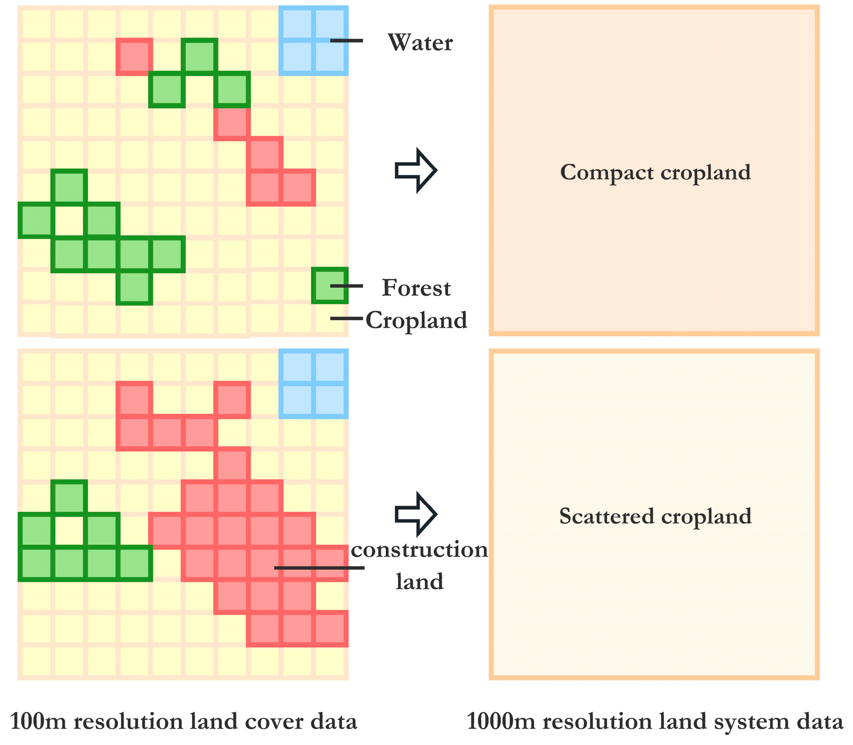
The proportion of area of land use/cover types in the image element characterizes land use intensity in this study. We produced a land system considering land use intensity based on two different resolutions of land use/cover type data (100 m and 1 km) (Figure 2). This land system can reflect land use/cover types and different land use intensities. For example, we first calculated the proportion of cropland pixels at 100 m resolution in the 1 km cropland pixel. Then we used the natural breakpoint method to divide the cropland at 1 km resolution into high-density and low-density cropland. Above the natural breakpoint division line is high-density and below it is low-density, as shown in Figure 3.

2.2.3. Driving Factors

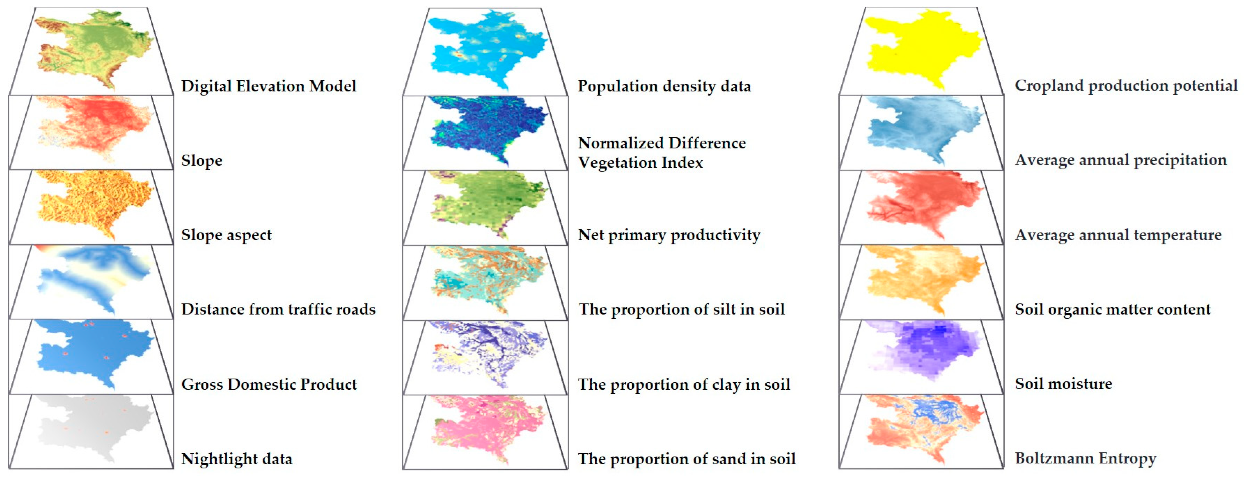
The driving factors of land change were selected according to two criteria: representativity and diversity, and data availability. As a result, we chose 18 driving factors, including 4 socio-economic and 13 natural-environmental driving factors, as seen in Table 1 and Figure 4. All driving factors were treated at a uniform spatial resolution of 1 km.

3. New Method, Evaluation, and Application

3.1. Improved CLUMondo with MaxEnt and Boltzmann Entropy

3.1.1. Overall Framework

In this study, we improve upon the CLUMondo land change model by integrating the MaxEnt model and Boltzmann entropy:
(1)
For the regression’s accuracy, we use the MaxEnt model to replace the logistic regression built into the CLUMondo model to improve the regression’s accuracy.
(2)
For spatial heterogeneity, we computed Boltzmann entropy based on DEM data as an additional driver factor of spatial heterogeneity.
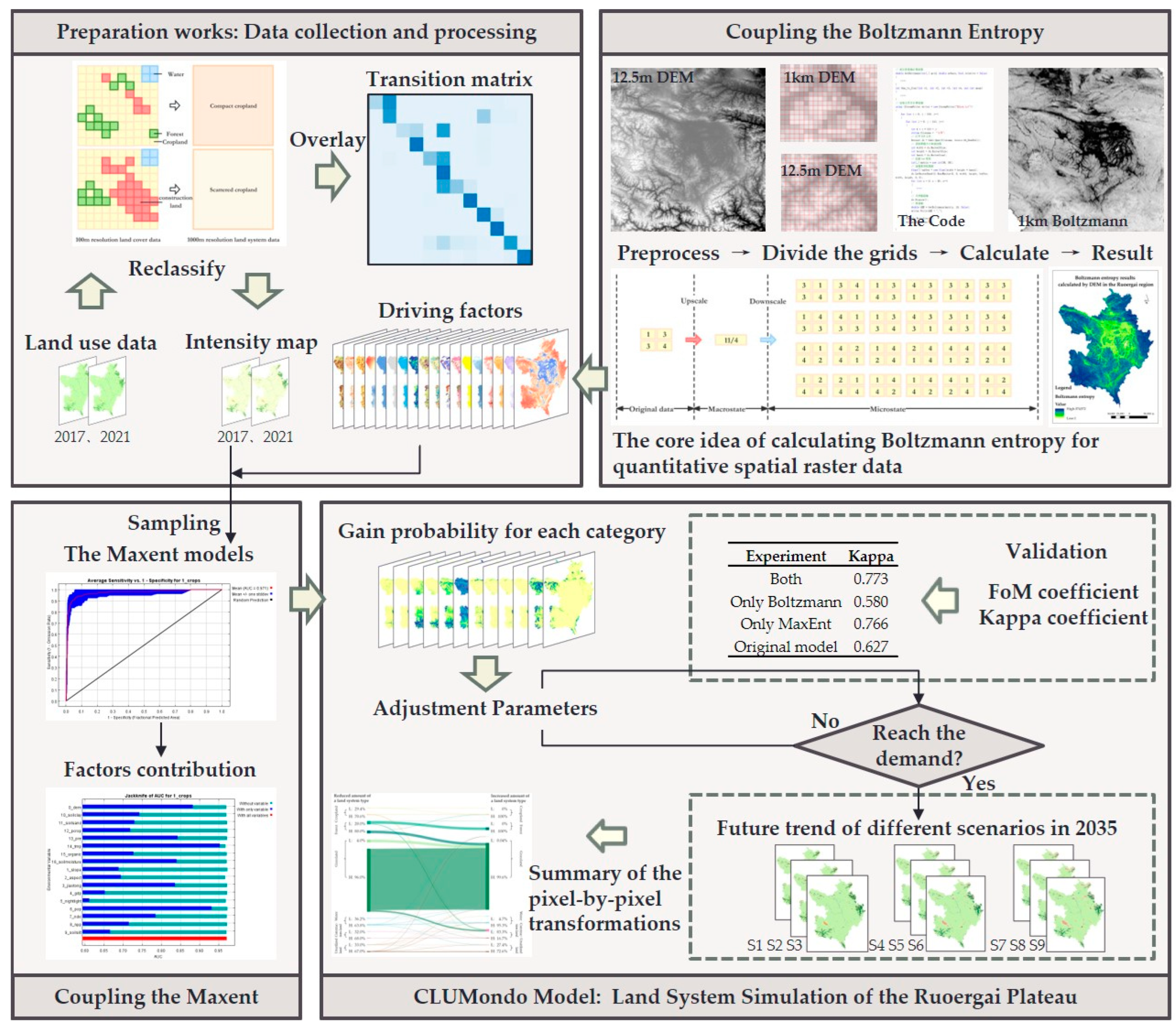
This study also considered land use intensity and proposed a novel integrated land use simulation model. Figure 5 shows the overall framework of the integrated model. Figure 6 shows the main work of this study.

3.1.2. CLUMondo Model

The CLUMondo model was developed by van Asselen and Verburg [38] based on CLUE (conversion of land use and its effects). The model consists of both demand and distribution modules.
The user inputs data on the current spatial distribution of the land system and future land demand. Under some internal mechanisms, the model iterates, configures and updates the spatial distribution data of the land system that are input by the user. The result is an expected spatial distribution of the land system that meets the user’s future demand.
CLUMondo is essentially an empirical demand-side statistical model. The imbalance between “supply” and “demand” motivates land transformation in the simulation process. The interpretation is that there is an imbalance between the supply provided by the current land system and the demand set by the users. If the bid-ask spread exceeds a certain threshold, the demand will cause the land to change until the equilibrium between supply and demand is reached, and the iteration stops. The model is based on the discrete-time step method, which considers space policy constraints, specific parameters of land use conversion, land use needs, and driver location characteristics to allocate land use optimally [38].

3.1.3. MaxEnt Model

Jaynes first proposed the MaxEnt principle based on Shannon’s notion of information entropy [58]. Phillips et al. proposed the MaxEnt model (MaxEnt) based on the principle of maximum information entropy and developed a software package for the MaxEnt model (MaxEnt 3.4) [59]. The central idea of the MaxEnt principle is that in estimating the posterior probability distribution from the prior probability information, we assume that the unknown information conforms to a uniform distribution. In this way, the conditional entropy of the system is maximized while the constraints are satisfied, i.e., the probability distribution of the system in the most durable case.
This paper calculated the probability distributions of various land types using the MaxEnt model with 18 drivers of land use change, such as DEM, average annual precipitation, and population density data as constraints.
H ( Y | X ) = i = 1 n P ( x i ) j = 1 m P ( y j | x i ) log P ( y j | x i )
where Y is the set of land use types, y i is each of the land use types, X is the set of driving factors, and x i is each of the driving factors.
The output of the MaxEnt model is the probability distribution of the different types of land use. We used the output probability file from the MaxEnt model instead of the probability file generated by the logistic regression built into the CLUMondo model.

3.1.4. Boltzmann Entropy

The driving factors used in previous studies applying the CLUMondo model seldom consider spatial heterogeneity within the pixels. In the study of complexity geography, the Boltzmann entropy of landscape gradients can be calculated to characterize spatial heterogeneity [46]. The Boltzmann entropy is chosen for two reasons. Firstly, it is theoretically able to characterize the constituent and configurational disorder of a system, whereas Shannon entropy can characterize only one of these at a time. In this sense, Boltzmann entropy is more suitable for landscape representation, where both composition and configuration are important. Second, Boltzmann entropy is thermodynamic entropy, which is key to explaining landscape ecological processes based on thermodynamic insights [46].
In this paper, we calculated the Boltzmann entropy of the DEM raster data. It is used to characterize spatial heterogeneity within raster data. We use the Boltzmann entropy driver as complementary to the CLUMondo model.
The Boltzmann entropy equation can be simplified by the following Equation (2):
S = k B log ( W )
where S is the Boltzmann entropy of the system; W is the number of microstates corresponding to the microstate; and k B is the Boltzmann constant, which takes the value of 1.3807 × 10⁻²³ J/K.
The method for computing the Boltzmann entropy of a landscape gradient was initially proposed by Gao et al. [60]. The method establishes the connection between macroscopic and microscopic states through scale transformation. Figure 7 illustrates the core idea of calculating Boltzmann entropy for quantitative spatial raster data. This method uses a 2 × 2 sliding window to compute the raster data. For each calculation, we derive the macroscopic (maximum, minimum, average, or sum) parameters for each window and the number of microstates corresponding to the case in which macroscopic parameters are constrained. The Boltzmann entropy of all raster data is computed by adding the number of microstates obtained from each sliding window in Equation (2). The strategy and improvement points of our coupling model can also be shown in Figure 6.
We use two different resolutions of DEM data (1 km and 12.5 km) and the method proposed by Gao et al. [46] to compute the Boltzmann entropy driving factor with a resolution of 1 km. The steps of computation are as follows, which are also illustrated in the “Coupling the Boltzmann Entropy” part in Figure 6.
  • Step 1: Splitting the Raster
Each 1 km pixel contains 80 × 80 12.5 m pixels. We calculated the Boltzmann entropy once for each 80 × 80 12.5 m pixels to represent the spatial heterogeneity of its corresponding 1 km pixel. ArcGIS is used to partition the 12.5 m raster data based on the 1 km pixel boundaries. We then obtain matrixes of 80 × 80 12.5 m pixels within each 1 km pixel.
  • Step 2: Cyclic Calculation
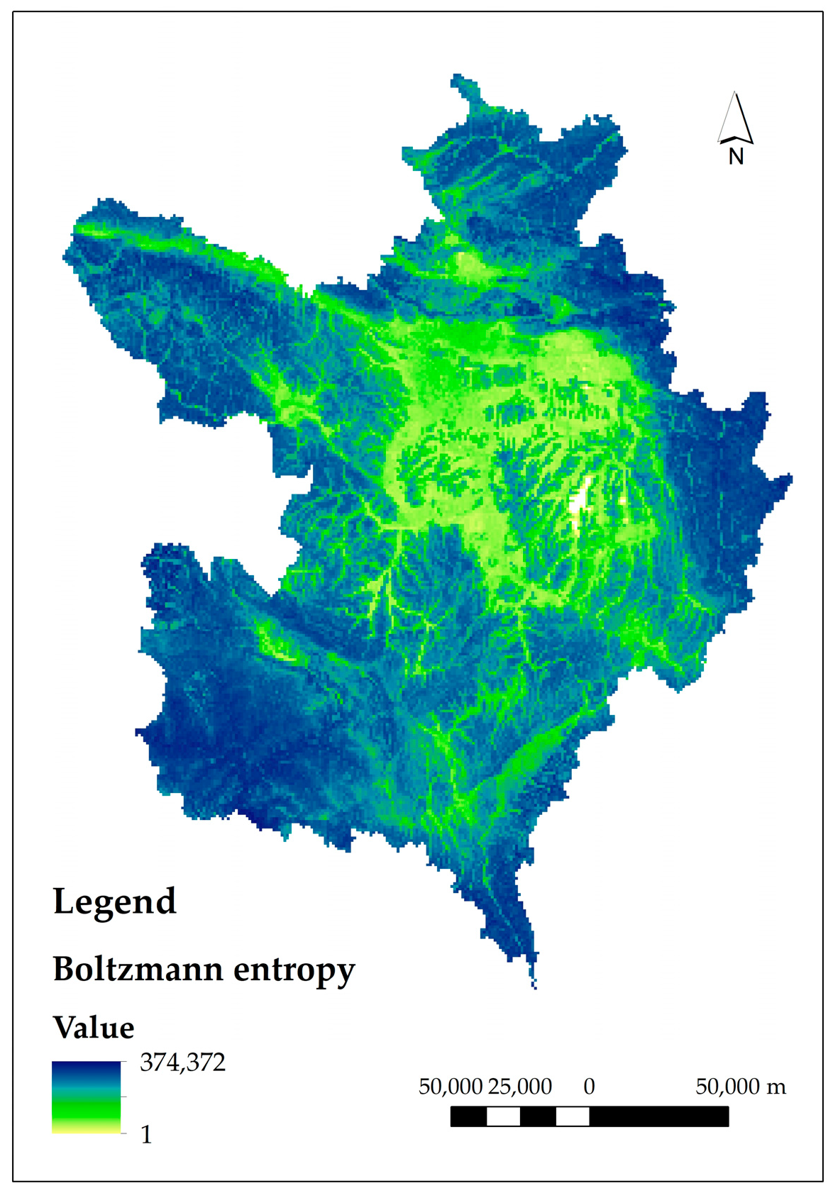
We used C# to compute the Boltzmann entropy of all 80 × 80 12.5 m DEM data in a cyclic manner, and then wrote the results in the Boltzmann entropy calculation result matrix. Finally, we obtained the Ruoergai Plateau’s total Boltzmann entropy driving factor with 1 km resolution, as shown in Figure 8.

3.2. Evaluation

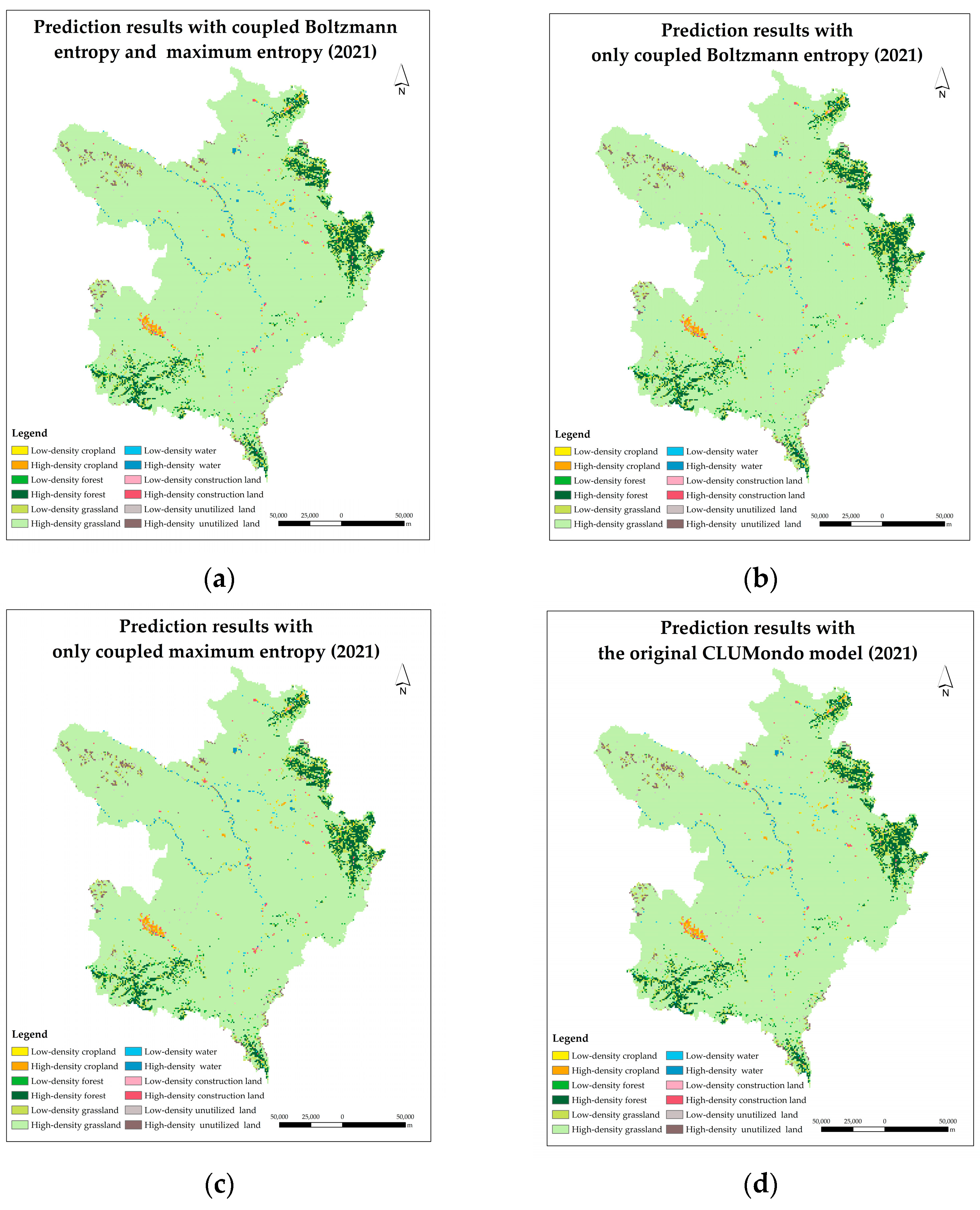
To evaluate the accuracy of the integrated model, we used the land system in 2017 to predict the land system in 2021. We took the prediction results and compared them with the existing land system in 2021. Table 2 and Figure 9 show the results of model evaluation. In the four models, the model integrated MaxEnt and Boltzmann entropy to achieve the highest accuracy, with a Kappa of close to 0.8.

3.3. Application

Next, we applied the improved CLUMondo model to future land system predictions on the Ruoergai Plateau. This study calculated the ecological and economic benefits of each type of land per unit area. Secondly, we set nine scenarios for the future development of the Ruoergai Plateau, with different ecological and economic benefit demands. The necessary parameter settings for the model iteration were also set.

3.3.1. Benefit Coefficients Calculation

In this study, the improved CLUMondo model was used to project the land use status of the study area in 2035, considering the different economic and ecological benefit growth needs. To quantitatively measure the growth of economic (GDP) and ecological benefits (GEP), the coefficient of ecological benefits (E) and the coefficient of economic benefits (D) were calculated in this paper:
G D P = i = 1 n D i
G E P = i = 1 n E i
where i represents the different land use types. The land use intensity was also considered, and the ecological and economic efficiency coefficients were calculated to consider the intensity of the land use.
  • Ecological efficiency coefficient (E)
The computation of the ecological efficiency coefficient is grounded in a theoretical examination of national-scale ecosystem service valuation. Table 3 of the Ecological Service Value Equivalents per Unit Area of Terrestrial Ecosystems in China [61] is the primary reference in this calculation. In addition, we also refer to the area of land use types at the municipal scale for the statistics of Gansu and Sichuan provinces.
When calculating the ecological efficiency factor, the economic value of annual natural food production on 1 hectare of cropland with the national average yield is defined as 1. The economic value of food production services provided by cropland ecosystems is equivalent to 1/7 of the market value of the national average food yield. The value equivalent factor of ecological services in other ecosystems is determined based on the contribution of each ecological service in comparison to the food production services of cropland [61]. This calculation can be expressed as follows:
Step 1: Calculate the economic value of food production services E a provided per unit of agroecosystem:
E a = 1 7 i = 1 n p Q i M
where M is the sum of sown area of food crops in five counties (km2), P is the price of grain (RMB/t), Q i is the grain production of a particular county (t), and E a is the sum of the economic value of five counties (million RMB), combined with the statistical bulletin of national economic and social development of Ruoergai counties in 2021.
E a is calculated in Table 4, which is 56,626 RMB/km2.
Step 2: Calculate the ecological efficiency coefficient E i :
E i = E a × k i
The ecological service value per unit area, denoted as k i , is crucial in the calculation. For instance, Table 3 provides the ecological service value per unit area of cropland as 6.91. By multiplying this value with the economic value of food production services, which is 56,626 RMB/km2 from Step 1, the ecological efficiency coefficient of cropland can be determined as 391,288 RMB/km2, as indicated in Table 5.
  • Economic Benefit Coefficient (D)
The economic coefficient was obtained by calculating the GDP generated from different land use types, as reported in the Statistical Yearbook of Sichuan Province for 2021, to the corresponding areas of each land use type (Table 6).
  • Calculation results in the economic benefit coefficient and ecological benefit coefficient
The results of the calculation of the economic and ecological efficiency coefficients for each land type on the Ruoergai Plateau are shown in Table 5.
Among them, construction land is a manufactured surface. It does not exist as a type of ecosystem services, so it is considered that construction land is incapable of providing ecosystem services. There is no value of ecosystem services, so the coefficient of ecological efficiency of construction land is set to 0. Unutilized land refers to land that cannot be developed and used by humans. There is no economic benefit or value of ecosystem services. Hence, the coefficients of economic and ecological benefits of unutilized land are both 0.
  • Ecological benefit and economic benefit coefficients that take into account land use intensity
Considering the intensity of land use, it is necessary to characterize land’s ecological and economic benefits based on the actual percentage of land use/cover types in the image element:
G E P I = i E i × area i
G D P I = i D i × area i
where G E P I is the ecological efficiency coefficient of a particular land use/cover type, G D P I is the economic efficiency coefficient of a particular land use/cover type; area i is the actual share of that land use/cover type; G E P I is the modified ecological efficiency coefficient, and G D P I is the modified economic efficiency coefficient. The results are shown in Table 7.
The product of the benefit coefficient of each type of land use and the area of each type of land is the ecological benefit of that type of land use. The ecological benefit in 2021 is 11,095,795 RMB, and the economic benefit is 4,963,351 RMB.

3.3.2. Future Scenarios Settings

This study establishes three GDP growth scenarios (12.6%, 63.0%, 126.1%) and three GEP growth scenarios (0.3%, 1.3%, 2.5%). By combining these scenarios, a total of nine demand scenarios are generated, as shown in Table 8.
Regarding economic benefit growth, we referenced the 14th Five-Year Plan (2020–2025) issued by Aba Prefecture and Gannan Prefecture governments. According to the plan, the expected annual GDP growth rate for Gannan Prefecture is 6%, while Aba Prefecture has a GDP annual growth rate of 6.5%. Based on a calculated GDP annual growth rate of 6%, the projected GDP increase in 2035 compared to 2021 is estimated to be 126.1%. If the plan is 50% achieved, the increase would be 63.0%; if it is 10% achieved, the increase would be 12.6%.
Regarding ecological benefit growth, we calculated the average annual GEP growth rate based on the land system in 2017 and the existing land system in 2021, which is determined to be 0.2%. Assuming this growth rate continues, the projected GEP increase in 2035 compared to 2021 would be 2.50%. If the target is 50% achieved, the increase would be 1.25%; if it is 10% achieved, the increase would be 0.25%.

3.3.3. Other Parameter Settings

In addition to the initial land system and projected land demand for the target year, the input parameters of the CLUMondo model also include conversion resistance and a transition matrix. The specific methods for setting the conversion resistance and transition matrix in this study are as follows:
  • Conversion Resistance
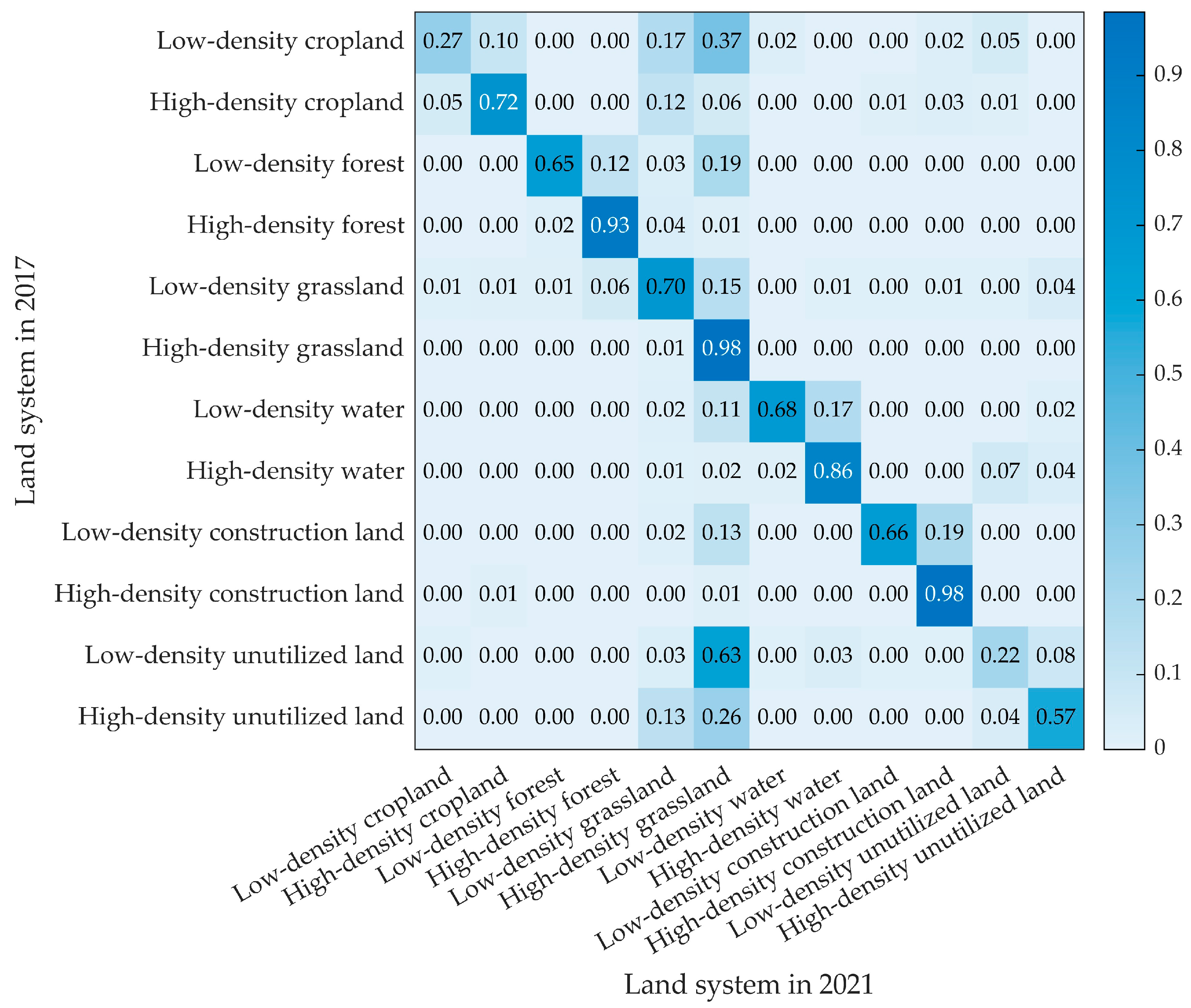
To calculate the conversion resistance values for each land use type, we initially computed the confusion matrix for the land system in 2017 and 2021 using the land use/cover intensity data of those respective years (Table 9; Figure 10). Subsequently, the conversion resistance values for each land use type were determined by dividing the number of unconverted rasters for a particular land use type by the total number of original rasters corresponding to that land use type (as shown in Table 9).
To present the results more clearly, we define low-density cropland, high-density unutilized land and so on, as numbers 0 to 11, respectively.
The conversion resistance value, denoted as r i , for land system type i is given by:
r i = 1 p i
where p i represents the probability of land system type i in 2017 being converted to other land system types in 2021. The results are shown in Table 10.
  • Transfer Matrix
The land use type transfer matrix represents the degree of ease in converting one land use type to another, with values ranging from 0 to 1. A value closer to 1 indicates a higher likelihood of conversion to the specific land use type, while a value closer to 0 suggests a lower likelihood.
In the setting of the transition matrix, a threshold of 0.1% is applied. If there has been a historical conversion between two land use types, the corresponding entry in the transition matrix is assigned a value of 1; otherwise, it is set to 0. Moreover, grassland can be converted to construction land, while water bodies exhibit low potential for conversion to forest or grassland. On the other hand, construction land is considered less prone to conversion into other land use types, thus assigned a value of 0, signifying its limited convertibility. The resulting transition matrix, outlined in Table 11, encapsulates these considerations.

4. Results

4.1. Land System Maps for Different Scenarios

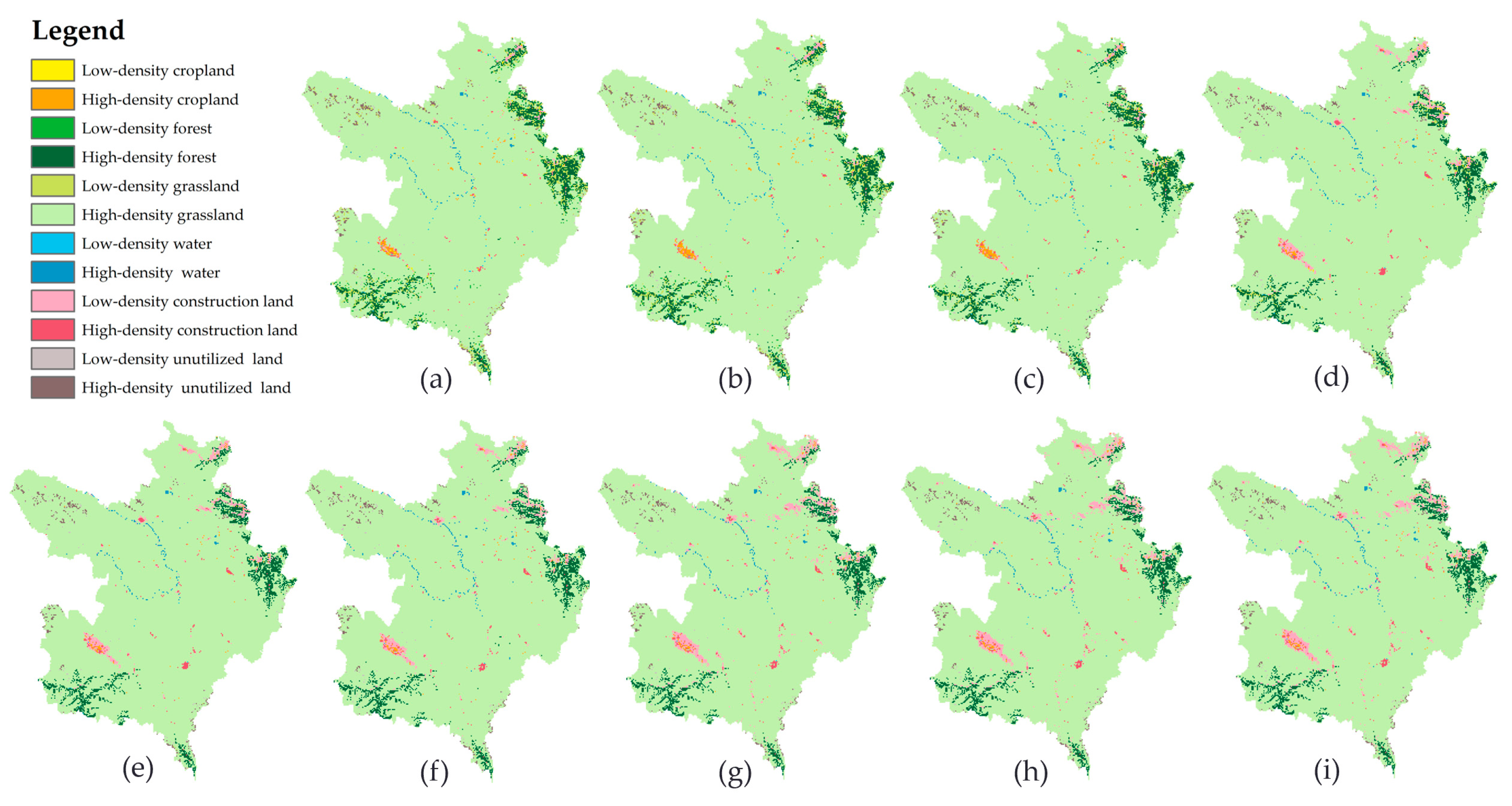
The improved CLUMondo model was used to project the land use types in the Ruoergai region in 2035. The results under nine future development scenarios (Table 8) are shown in Figure 11 and Table 12.
Two typical areas (in Figure 12) were selected: the central town area of Aba County and the lower elevation forest in the eastern part of Ruoergai County, which are shown in Figure 13 and Figure 14.
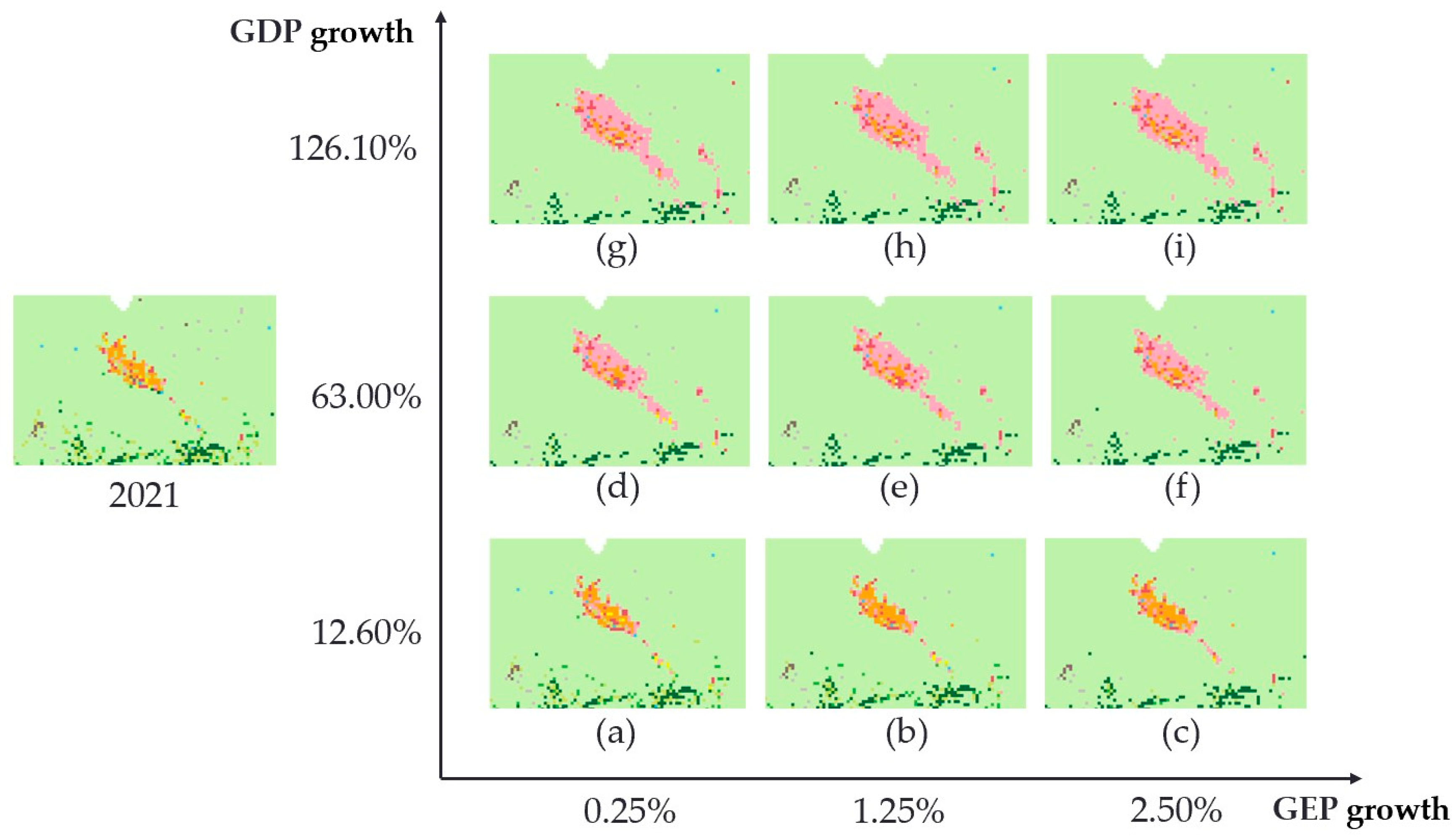
Comparing the subplots in Figure 12 horizontally, we can analyze the change in land use intensity with the increase in the ecological efficiency target when the economic efficiency is certain. Figure 13a–c present the change in land use intensity with increasing ecological efficiency target when the economic efficiency target is low: low-density cropland is converted to high-density cropland, and low-density grassland is converted to high-density grassland, while the increase in economic efficiency (Figure 13d–f) results in more conversion of cropland to urban land and conversion of low-density grassland to high-density grassland. It is known from Figure 13g–i that the expansion of construction land will reach saturation as economic efficiency objectives reach a certain level.
While vertically comparing the subplots in Figure 12, we can analyze the change of land use intensity with the increase in the economic benefit target when the ecological benefit is certain. Subplots Figure 13a–i show similar patterns of change: (1) in terms of type change, cropland and grassland are converted to construction land, and towns show a trend of expansion; (2) in terms of utilization intensity, low-density cropland is converted to high-density cropland, low-density grassland and forest are converted to high-density grassland, and low-density construction land is converted to high-density construction land; (3) in terms of distribution location, there are new town points, indicating that this area may be suitable for town development. In addition, Figure 13c,f,i show that there is a lateral evolution of construction land from linear to faceted distribution as the economic efficiency target increases.
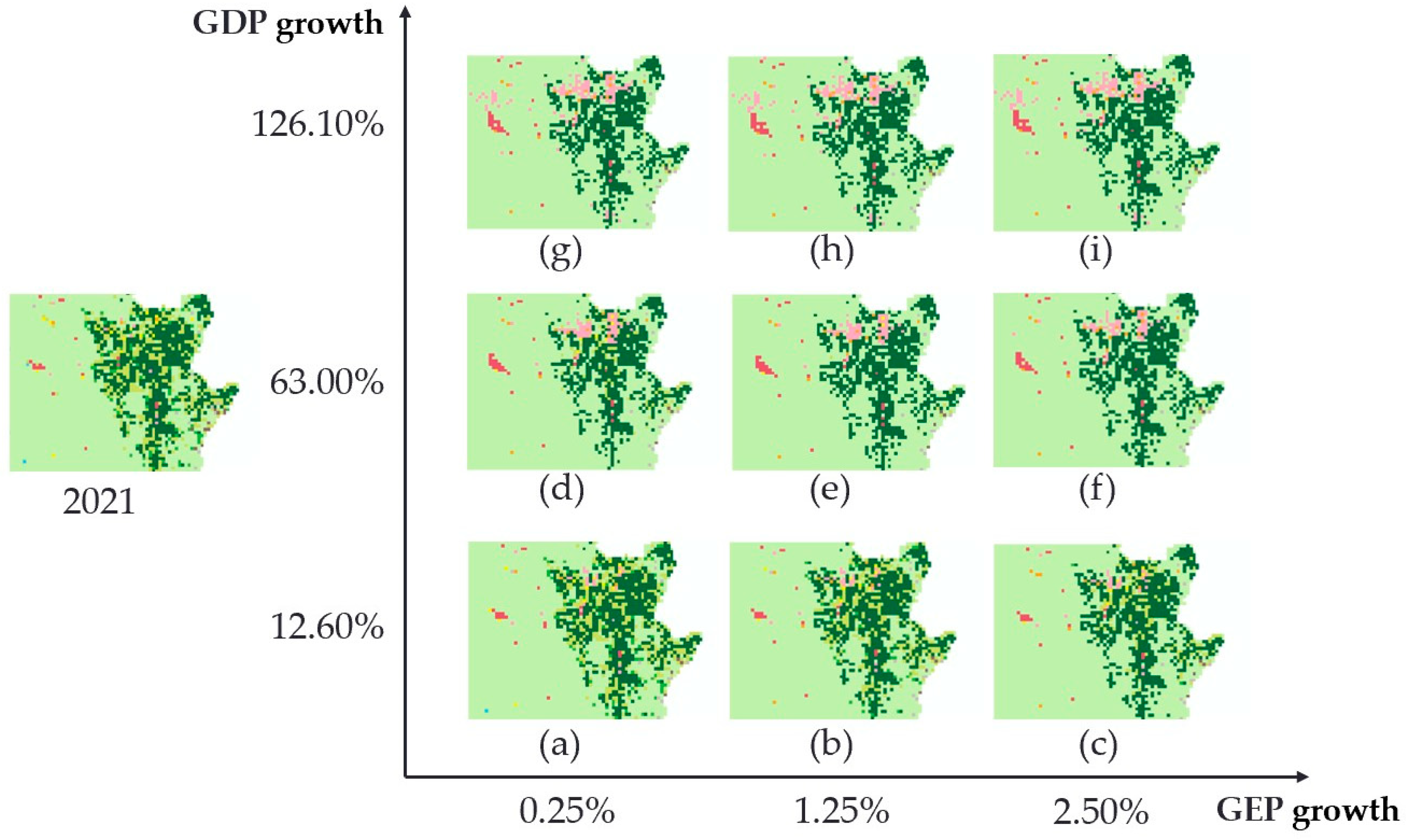
A horizontal look at subplots Figure 14a–c shows that as the ecological efficiency target increases there is a conversion of low-density forest to high-density forest and low-density grassland to high-density grassland. And according to Figure 14d–f, it is known that there is a more significant increase in forest area with the increase in the ecological efficiency target.
Vertically, the change of land use with increasing economic efficiency targets are as follows: (1) in terms of type, forest and grassland are converted to construction land, and towns show expansion trend; (2) in terms of utilization intensity, low-density cropland is converted to high-density cropland, low-density forest is converted to high-density forest, and low-density grassland is converted to high-density grassland.
Overall, Figure 13 and Figure 14 show that: (1) with the increase in demand for ecological benefits, there is little change in land use types. But regarding utilization intensity, land use intensity shows an apparent increasing trend. For example, low-density cropland is transformed into high-density cropland, low-density grassland is transformed into high-density grassland, low-density forest is transformed into high-density forest, etc.; (2) with the increase in demand for economic benefits, the area of construction land significantly increases in terms of land use type, while the area of cropland decreases. In terms of intensity, the intensity of utilization of construction land, unutilized land, forest, and grassland all increase significantly. Regarding spatial distribution, the construction land area expands toward the plain area in the central part of Ruoergai County.

4.2. Analysis of Land System Type Transitions

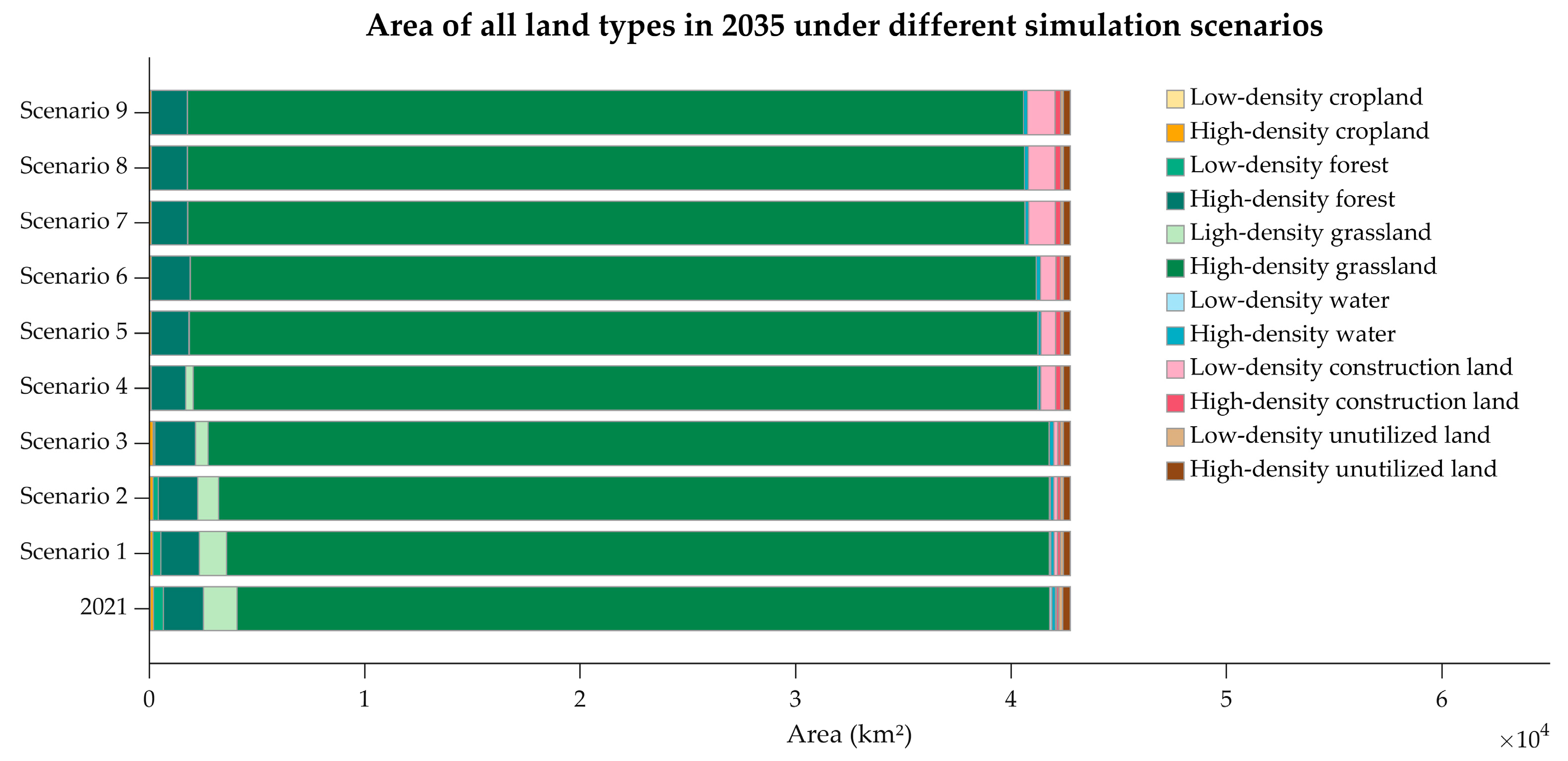
The areas of land use types on the Ruoergai Plateau in 2035 under different scenarios in Figure 11 were measured and plotted in Figure 15 and Figure 16.
By Figure 15 and Figure 16 it can be seen that when the demand for economic benefits is the same (scenarios 1, 2, 3; scenarios 4, 5, 6; scenarios 7, 8, 9), the total area of water shows an apparent increasing trend in terms of the change of land use type as the demand for ecological benefits increases, and grassland and cropland are partially transformed into water. Although the total area of cropland, forest, construction land, and grassland fluctuates, the intensity of land use shows an increasing trend in terms of land use intensity, i.e., from low-density cropland to high-density cropland and low-density grassland to high-density grassland, and the degree of land use intensification increases significantly. The unutilized land is more difficult to develop due to severe natural conditions and other restrictions, and the overall change in area is minimal.
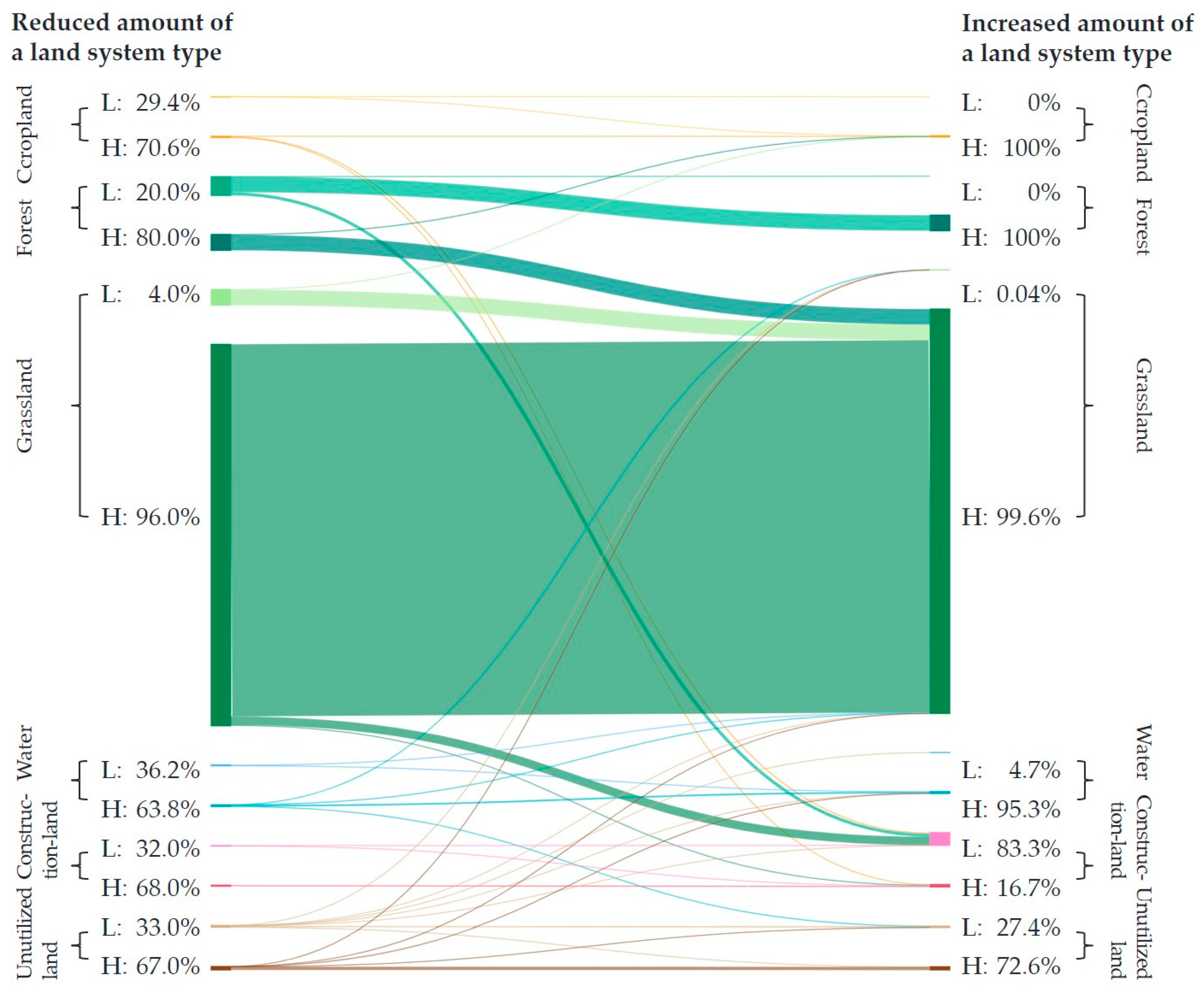
With the same demand for ecological benefits (scenarios 1, 4, 7; scenarios 2, 5, 8; scenarios 3, 6, 9), the total area of construction land shows a noticeable trend of increase in terms of changes in land use/cover types as the demand for economic benefits increases, and grassland, forest, and cropland are partially converted into construction land, which is consistent with the higher economic benefits of construction land. The prediction results show that with the increase in economic benefit demand, the construction land is expands primarily around the original towns and cities, and new construction land gathering areas appear in the lower elevation areas near the mountains of Ruoergai, which is of great significance for guiding the location of towns and cities and urban construction. In terms of land use intensity, there is a significant trend of increasing land use intensity; for example, low-density construction land is mainly converted into high-density construction land and low-density cropland is converted into high-density cropland. High-density construction land can accommodate more people and generate more economic benefits per unit area than low-density construction land; high-density cropland can provide more crop output per unit area than low-density cropland. More precisely, in scenario 9, among the “grassland” sources, 96.0% of the area (37,632 km2) comes from the high-density category (Figure 17) and 4.0% of the area is low density; overall, 0.103% of the area of this source will convert into high-density cropland and 2.35% of the area of this source will convert into construction land.
Compared with the interconversion between various land use types when intensity is not considered, the simulation of land use/cover change with consideration of land use intensity can better determine the conversion within the same land use type, and thus can simulate the actual changes under different demand scenarios in a more refined and reasonable way.

5. Discussion

In this section, we discuss previous research on the Ruoergai Plateau and the contributions of this study. Then we reflect on the limits of our study and look ahead. Finally, we put forward our policy recommendations based on this study.
Previous studies of the Ruoergai Plateau have included methane production potential, soil organic carbon, organochlorine pesticides and polychlorinated biphenyls (PCBs), land desertification and degradation, seismic reflection, ecosystem services and so on [62,63,64,65,66,67]. Based on the improved CLUMondo model, this study predicts 2035 land transformation on the Ruoergai Plateau, which is rare in previous studies.
We used an integrated CLUMondo model to build nine scenarios, which is a highlight of this study. The improved CLUMondo model is based on the driving factors of the land system to derive the suitability of land. It used two-time points of service demand to pull the model iteration. However, there are limitations to this approach. First, using only ecological and economic efficiency may simplify future modeling, for example, by failing to consider resource efficiency [68]. Secondly, this future scenario is based on hypothetical economic growth rates and ecological efficiency growth rates for existing years (2017 and 2021). There are too many implemented factors for the model and focusing mainly on economic and ecological benefits is too simple. It does not represent absolute future results and may differ from actual developments. As a result, the results of this study may be uncertain, and evaluation through field studies and more detailed resolution assessments will enhance the study’s evaluation when time and data are available. In addition, the robustness of the model has not been proved. Land types that considered intensity were likely to have lower Kappa than land types that did not consider intensity. It can be used to predict the whole area and even the broader area of the Tibetan Plateau and can be used as a reference for constructing and protecting measures according to local conditions.
To better balance the ecological protection and economic development of the Tibetan Plateau region, the following countermeasures are proposed according to the simulation results for different future needs:
(1)
To meet economic development needs, the amount of land used for construction needs to be increased substantially.
Comparing the current situation in 2021 with the spatial distribution of projected results in 2035, the low-density construction land in the nine scenarios was mostly replaced by high-density construction land, and the low-density cropland was mostly replaced by high-density cropland.
(2)
Optimizing the development structure for construction land and cropland.
According to the simulation results, to achieve economic benefits, the land use intensity of cropland and construction land is increasing, which shows that the current construction land and cropland have the potential to develop in a more intensive direction. The development of construction land and cropland should focus more on the intensity of development rather than the proportion of the two areas. This can effectively solve the problem of irrational utilization and exploitation of limited land resources caused by the conflict between cropland and construction land. Therefore, it is beneficial to bring into play the ecological value of the Ruoergai Plateau as an important water conservation ecological function area in the upper reaches of the Yellow River and to maintain a more stable ecological balance.
(3)
The central plain of Aba County and the northwest of Ruoergai County are suitable for town selection and urban construction.
According to the spatial distribution of the simulation results, the increase in high-density construction land in 2035 is concentrated in the low plain of Aba County and the northwest of Ruoergai County. The high-density cropland and high-density construction land in these areas show the characteristics of centralized distribution and low heterogeneity of internal space. Therefore, to develop the economy with ecological considerations as far as possible, priority should be given to the development of such areas so that unnatural areas of the Ruoergai Plateau can be utilized to a certain extent for regional development.

6. Conclusions

This study improves the CLUMondo land change simulation model by integrating the MaxEnt model and Boltzmann entropy. The enhanced model simulates land use changes in Ruoergai grasslands of the Qinghai-Tibet Plateau. In addition to considering land use/cover changes, this study also incorporates changes in land use intensity.
The accuracy evaluation of the model involves four sets of comparative experiments. In the four models, the model integrated MaxEnt and Boltzmann entropy to achieve the highest accuracy, with a Kappa of 0.773.. Furthermore, the simulation results considering land use intensity changes are more refined than only considering land use/cover changes. Considering land use intensity changes can reflect the transformation processes between different intensities within the same land use type.
During the land use simulation of Ruoergai Grassland under nine different scenarios of ecological and economic benefits, the following findings are noted:
(1)
With increasing ecological benefit demands, the water area significantly increases, and the intensity of forest and grassland utilization shows an increasing trend. With 0.25% GDP growth, the water area is about 178 km2. With 2.5% GEP growth, the water area is about 202 km2. The latter is 24 km2 more than the former, which is about 13.6% greater. Low-density forest decreased by 82.2%, High-density forest increased by 6.0%, Low-density grassland decreased by 62.2%, and High-density grassland increased by 0.7%.
(2)
With increasing economic benefit demands, construction land and grassland utilization intensities increase. The plain area in the central part of Ruoergai County expands outward for construction land, and new clusters of construction land appear in the eastern region. With 12.6% GDP growth, the High-density construction area is about 399 km2. With 126.1% GEP growth, the water area is about 761 km2. High-density construction land increased by 90.7% (about 362 km2) and High-density grassland increased by 0.6% (about 30 km2).
In future research, expanding the intensity levels of land use, such as subdividing cropland into low-density, medium-density and high-density categories, is recommended. This refinement would allow for more detailed simulation results, enabling a better understanding of land use intensity variations. Additionally, expanding the study area and applying the improved integrated model to the entire Qinghai-Tibet Plateau or even larger regions for land use simulation would be beneficial. This broader scope would provide a more comprehensive analysis of land use dynamics and their implications on a larger spatial scale.

Author Contributions

Conceptualization, Z.S., Y.W., J.L. and P.G.; methodology, Z.S., Y.W. and J.L.; software, Z.S., Y.W. and J.L.; validation, Z.S.; formal analysis, Z.S. and Y.W.; investigation, Z.S.; resources, Z.S.; data curation, Z.S. and J.L.; writing—original draft preparation, Z.S., Y.W. and J.L.; writing—review and editing, P.G.; visualization, Z.S., Y.W. and J.L.; supervision, P.G.; project administration, Z.S. and P.G.; funding acquisition, P.G. All authors have read and agreed to the published version of the manuscript.

Funding

This research has been supported by the National Natural Science Foundation of China (Grant Nos. 42271418, 42230106, 42171088, and 42171250) and State Key Laboratory of Earth Surface Processes and Resource Ecology (Grant No. 2022-ZD-04).

Data Availability Statement

The global land cover map with a 10 m resolution generated from Sentinel-2 satellite data acquired from Esri Releases New 2020 Global Land Cover Map (https://www.esri.com/about/newsroom/announcements/esri-releases-new-2020-global-land-cover-map/ (accessed on 24 May 2023)). Most of the driving factors are from Resource and Environmental Science and Data Center (https://www.resdc.cn/data.aspx (accessed on 24 May 2023)). GDP data were acquired from Global 1 km × 1 km gridded revised real gross domestic product and electricity consumption during 1992–2019 based on calibrated nighttime light data (https://eogdata.mines.edu/nighttime_light/annual/v20/ (accessed on 24 May 2023)). Nightlight data were acquired from EOG Nighttime Light (http://www.glass.umd.edu/NPP/AVHRR/GLASS_NPP_005D_YEAR/2015/ (accessed on 24 May 2023)). Population density data were acquired from Google Earth Engine Datasets (https://developers.google.com/earth-engine/datasets/catalog/WorldPop_GP_100m_pop (accessed on 24 May 2023)). NPP data were acquired from GLASS product (http://www.glass.umd.edu/NPP/AVHRR/GLASS_NPP_005D_YEAR/2015/ (accessed on 24 May 2023)). Average annual precipitation and Average annual temperature data were acquired from 1 km monthly temperature and precipitation dataset for China from 1901 to 2017 (https://doi.org/10.5194/essd-11-1931-2019 (accessed on 24 May 2023)). Soil moisture data are from A fine-resolution soil moisture dataset for China in 2002~2018 (https://doi.org/10.5281/zenodo.4738556 (accessed on 24 May 2023)).

Conflicts of Interest

The authors declare no conflict of interest.

References

  1. Turner, B.L.; Lambin, E.F.; Verburg, P.H. From land-use/land-cover to land system science. Ambio 2021, 50, 1291–1294. [Google Scholar] [CrossRef] [PubMed]
  2. He, C.; Zhang, J.; Liu, Z.; Huang, Q. Characteristics and progress of land use/cover change research during 1990–2018. J. Geogr. Sci. 2022, 32, 537–559. [Google Scholar] [CrossRef]
  3. Li, D.; Wang, L. Sensitivity of surface temperature to land use and land cover change-induced biophysical changes: The scale issue. Geophys. Res. Lett. 2019, 46, 9678–9689. [Google Scholar] [CrossRef]
  4. Heilmayr, R.; Echeverría, C.; Lambin, E.F. Impacts of Chilean forest subsidies on forest cover, carbon and biodiversity. Nat. Sustain. 2020, 3, 701–709. [Google Scholar] [CrossRef]
  5. Dimyati, M.U.H.; Mizuno, K.E.I.; Kobayashi, S.; Kitamura, T. An analysis of land use/cover change in Indonesia. Int. J. Remote Sens. 1996, 17, 931–944. [Google Scholar] [CrossRef]
  6. Thiery, W.; Davin, E.L.; Seneviratne, S.I. Land Use, Land Cover and Land Management Change: Definitions, Scenarios, and Role in the Climate System. In Oxford Bibliographies in Environmental Science; Oxford University Pres: Oxford, UK, 2018. [Google Scholar] [CrossRef]
  7. Kaul, H.A.; Sopan, I. Land use land cover classification and change detection using high resolution temporal satellite data. J. Environ. 2012, 1, 146–152. [Google Scholar]
  8. Comber, A.; Fisher, P.; Wadsworth, R. What is land cover? Environ. Plan. B Plan. Des. 2005, 32, 199–209. [Google Scholar] [CrossRef] [Green Version]
  9. Ito, A.; Hajima, T. Biogeophysical and biogeochemical impacts of land-use change simulated by MIROC-ES2L. Prog. Earth Planet. Sci. 2020, 7, 54. [Google Scholar] [CrossRef]
  10. Wardlow, B.D.; Egbert, S.L.; Kastens, J.H. Analysis of time-series MODIS 250 m vegetation index data for crop classification in the U.S. Central Great Plains. Remote Sens. Environ. 2007, 108, 290–310. [Google Scholar] [CrossRef] [Green Version]
  11. Kindu, M.; Schneider, T.; Teketay, D.; Knoke, T. Changes of ecosystem service values in response to land use/land cover dynamics in Munessa–Shashemene landscape of the Ethiopian highlands. Sci. Total Environ. 2016, 547, 137–147. [Google Scholar] [CrossRef]
  12. Wardlow, B.D.; Egbert, S.L. Large-area crop mapping using time-series MODIS 250 m NDVI data: An assessment for the U.S. Central Great Plains. Remote Sens. Environ. 2008, 112, 1096–1116. [Google Scholar] [CrossRef]
  13. Sohl, T.L.; Sleeter, B.M.; Zhu, Z.; Sayler, K.L.; Bennett, S.; Bouchard, M.; Reker, R.; Hawbaker, T.; Wein, A.; Liu, S.; et al. A land-use and land-cover modeling strategy to support a national assessment of carbon stocks and fluxes. Appl. Geogr. 2012, 34, 111–124. [Google Scholar] [CrossRef]
  14. Gao, P.; Gao, Y.; Ou, Y.; McJeon, H.; Zhang, X.; Ye, S.; Wang, Y.; Song, C. Fulfilling global climate pledges can lead to major increase in forest land on Tibetan Plateau. iScience 2023, 26, 106364. [Google Scholar] [CrossRef] [PubMed]
  15. Tewkesbury, A.P.; Comber, A.J.; Tate, N.J.; Lamb, A.; Fisher, P.F. A critical synthesis of remotely sensed optical image change detection techniques. Remote Sens. Environ. 2015, 160, 1–14. [Google Scholar] [CrossRef] [Green Version]
  16. Jain, A.K.; Meiyappan, P.; Song, Y.; House, J.I. CO2 emissions from land-use change affected more by nitrogen cycle, than by the choice of land-cover data. Glob. Chang. Biol. 2013, 19, 2893–2906. [Google Scholar] [CrossRef]
  17. Song, W.; Deng, X. Land-use/land-cover change and ecosystem service provision in China. Sci. Total Environ. 2017, 576, 705–719. [Google Scholar] [CrossRef]
  18. Sharma, R.; Nehren, U.; Rahman, S.A.; Meyer, M.; Rimal, B.; Aria Seta, G.; Baral, H. Modeling Land Use and Land Cover Changes and Their Effects on Biodiversity in Central Kalimantan, Indonesia. Land 2018, 7, 57. [Google Scholar] [CrossRef] [Green Version]
  19. Miranda, A.; Altamirano, A.; Cayuela, L.; Lara, A.; González, M. Native forest loss in the Chilean biodiversity hotspot: Revealing the evidence. Reg. Environ. Chang. 2017, 17, 285–297. [Google Scholar] [CrossRef]
  20. Patz, J.A.; Daszak, P.; Tabor, G.M.; Aguirre, A.A.; Pearl, M.; Epstein, J.; Wolfe, N.D.; Kilpatrick, A.M.; Foufopoulos, J.; Molyneux, D. Unhealthy landscapes: Policy recommendations on land use change and infectious disease emergence. Environ. Health Perspect. 2004, 112, 1092–1098. [Google Scholar] [CrossRef] [Green Version]
  21. Wu, J.; Sun, Z.; Yao, Y.; Liu, Y. Trends of Grassland Resilience under Climate Change and Human Activities on the Mongolian Plateau. Remote Sens. 2023, 15, 2984. [Google Scholar] [CrossRef]
  22. Yang, H.; Mu, S.; Li, J. Effects of ecological restoration projects on land use and land cover change and its influences on territorial NPP in Xinjiang, China. CATENA 2014, 115, 85–95. [Google Scholar] [CrossRef]
  23. Song, X.-P.; Hansen, M.C.; Stehman, S.V.; Potapov, P.V.; Tyukavina, A.; Vermote, E.F.; Townshend, J.R. Global land change from 1982 to 2016. Nature 2018, 560, 639–643. [Google Scholar] [CrossRef] [PubMed]
  24. Scanlon, B.R.; Reedy, R.C.; Stonestrom, D.A.; Prudic, D.E.; Dennehy, K.F. Impact of land use and land cover change on groundwater recharge and quality in the southwestern US. Glob. Chang. Biol. 2005, 11, 1577–1593. [Google Scholar] [CrossRef]
  25. Mooney, H.A.; Duraiappah, A.; Larigauderie, A. Evolution of natural and social science interactions in global change research programs. Proc. Natl. Acad. Sci. USA 2013, 110, 3665–3672. [Google Scholar] [CrossRef]
  26. Eitelberg, D.A.; van Vliet, J.; Doelman, J.C.; Stehfest, E.; Verburg, P.H. Demand for biodiversity protection and carbon storage as drivers of global land change scenarios. Glob. Environ. Chang. 2016, 40, 101–111. [Google Scholar] [CrossRef]
  27. Song, C.; Cheng, C.; Shi, P. Geography complexity: New connotations of geography in the new era. Acta Geogr. Sin. 2018, 73, 1204–1213. [Google Scholar]
  28. Foley, J.A.; Ramankutty, N.; Brauman, K.A.; Cassidy, E.S.; Gerber, J.S.; Johnston, M.; Mueller, N.D.; O’Connell, C.; Ray, D.K.; West, P.C.; et al. Solutions for a cultivated planet. Nature 2011, 478, 337–342. [Google Scholar] [CrossRef] [Green Version]
  29. Huajun, T.; Wenbin, W.U.; Peng, Y.; Youqi, C.; Peter, H.V. Recent Progresses of Land Use and Land Cover Change (LUCC) Models. Acta Geogr. Sin. 2009, 64, 456–468. [Google Scholar]
  30. Muller, M.R.; Middleton, J. A Markov model of land-use change dynamics in the Niagara Region, Ontario, Canada. Landsc. Ecol. 1994, 9, 151–157. [Google Scholar] [CrossRef]
  31. Portela, R.; Rademacher, I. A dynamic model of patterns of deforestation and their effect on the ability of the Brazilian Amazonia to provide ecosystem services. Ecol. Model. 2001, 143, 115–146. [Google Scholar] [CrossRef]
  32. Parker, D.C.; Manson, S.M.; Janssen, M.A.; Hoffmann, M.J.; Deadman, P. Multi-Agent Systems for the Simulation of Land-Use and Land-Cover Change: A Review. Ann. Assoc. Am. Geogr. 2003, 93, 314–337. [Google Scholar] [CrossRef] [Green Version]
  33. Valbuena, D.; Verburg, P.H.; Bregt, A.K.; Ligtenberg, A. An agent-based approach to model land-use change at a regional scale. Landsc. Ecol. 2010, 25, 185–199. [Google Scholar] [CrossRef] [Green Version]
  34. Li, X.; Yeh, A.G.-O. Cellular automata for simulating complex land use systems using neural networks. Geogr. Res. 2005, 24, 19–27. [Google Scholar] [CrossRef]
  35. Boissau, S.; Castella, J.-C. Constructing a common representation of local institutions and land use systems through simulation-gaming and multiagent modeling in rural areas of Northern Vietnam: The SAMBA-Week methodology. Simul. Gaming 2003, 34, 342–357. [Google Scholar] [CrossRef] [Green Version]
  36. Veldkamp, A.; Fresco, L.O. CLUE-CR: An integrated multi-scale model to simulate land use change scenarios in Costa Rica. Ecol. Model. 1996, 91, 231–248. [Google Scholar] [CrossRef]
  37. Verburg, P.H.; de Koning, G.H.J.; Kok, K.; Veldkamp, A.; Bouma, J. A spatial explicit allocation procedure for modelling the pattern of land use change based upon actual land use. Ecol. Model. 1999, 116, 45–61. [Google Scholar] [CrossRef]
  38. Van Asselen, S.; Verburg, P.H. Land cover change or land-use intensification: Simulating land system change with a global-scale land change model. Glob. Chang. Biol. 2013, 19, 3648–3667. [Google Scholar] [CrossRef]
  39. Gao, P.; Gao, Y.; Zhang, X.; Ye, S.; Song, C. CLUMondo-BNU for simulating land system changes based on many-to-many demand–supply relationships with adaptive conversion orders. Sci. Rep. 2023, 13, 5559. [Google Scholar] [CrossRef]
  40. Kakouei, K.; Kraemer, B.M.; Anneville, O.; Carvalho, L.; Feuchtmayr, H.; Graham, J.L.; Higgins, S.; Pomati, F.; Rudstam, L.G.; Stockwell, J.D.; et al. Phytoplankton and cyanobacteria abundances in mid-21st century lakes depend strongly on future land use and climate projections. Glob. Chang. Biol. 2021, 27, 6409–6422. [Google Scholar] [CrossRef]
  41. Malek, Z.; Verburg, P.H.; Geijzendorffer, I.R.; Bondeau, A.; Cramer, W. Global change effects on land management in the Mediterranean region. Glob. Environ. Chang.-Hum. Policy Dimens. 2018, 50, 238–254. [Google Scholar] [CrossRef] [Green Version]
  42. Gao, P.; Xie, Y.; Song, C.; Cheng, C.; Ye, S. Exploring detailed urban-rural development under intersecting population growth and food production scenarios: Trajectories for China’s most populous agricultural province to 2030. J. Geogr. Sci. 2023, 33, 222–244. [Google Scholar] [CrossRef]
  43. Zhang, Y.; Liu, X.; Chen, G.; Hu, G. Simulation of urban expansion based on cellular automata and maximum entropy model. Sci. China Earth Sci. 2020, 50, 339–352. [Google Scholar] [CrossRef]
  44. Zhang, J.; Chen, Y.; Yang, X.; Qiao, W.; Wang, D. The Demarcation of Urban Development Boundary Based on the Maxent-CA Model: A Case Study of Wuxi in China. Sustainability 2022, 14, 11426. [Google Scholar] [CrossRef]
  45. Gao, P.; Zhang, H.; Jia, D.; Song, C.; Cheng, C.; Shen, S. Efficient Approach for Computing the Discrimination Ratio-Based Variant of Information Entropy for Image Processing. IEEE Access 2020, 8, 92552–92564. [Google Scholar] [CrossRef]
  46. Gao, P.; Li, Z. Computation of the Boltzmann entropy of a landscape: A review and a generalization. Landsc. Ecol. 2019, 34, 2183–2196. [Google Scholar] [CrossRef]
  47. Sichuan Provincial Finance Department. Some Protection and Restoration of Ecological Management Budget (Provincial) Notify the Financial Department of Sichuan Province Natural Resources in Sichuan Province about Released in 2023, 2. Available online: http://czt.sc.gov.cn/scczt/c102423/2023/1/28/4a3004667e504d8eaea17c349d610170.shtml (accessed on 24 May 2023).
  48. The People’s Government of Aba Tibetan Qiang Autonomous Prefecture. Aba Tibetan and Qiang Autonomous Prefecture, Aba Prefecture People’s Government about Print and Distribute the Fourteenth National Economic and Social Development Five-Year Plan and 2035 Vision Compendium of Notice. Available online: https://www.abazhou.gov.cn/abazhou/c102077/202103/598d763b5bab4cfa98cbdb86acdfd778.shtml (accessed on 24 May 2023).
  49. The People’s Government of Ganzi Tibetan Autonomous Prefecture. The 14th Five-Year Plan for National Economic and Social Development of Garze Tibetan Autonomous Prefecture and the Outline of the Long-Range Goals to 2035. Available online: http://www.gzz.gov.cn/ghxxfzgh/article/63726 (accessed on 24 May 2023).
  50. Xiang, S.; Guo, R.; Wu, N.; Sun, S. Current status and future prospects of Zoige Marsh in Eastern Qinghai-Tibet Plateau. Ecol. Eng. 2009, 35, 553–562. [Google Scholar] [CrossRef]
  51. Gong, P.; Liu, H.; Zhang, M.; Li, C.; Wang, J.; Huang, H.; Clinton, N.; Ji, L.; Li, W.; Bai, Y.; et al. Stable classification with limited sample: Transferring a 30-m resolution sample set collected in 2015 to mapping 10-m resolution global land cover in 2017. Sci. Bull. 2019, 64, 370–373. [Google Scholar] [CrossRef]
  52. Xu, X.; Liu, J.; Zhang, S.; Li, R.; Yan, C.; Wu, S. Remote Sensing Data Set of Multi-Period Land Use Monitoring in China; Resource and Environmental Science Data Center: Beijing, China, 2018. [Google Scholar] [CrossRef]
  53. Chen, J.; Gao, M.; Cheng, S.; Hou, W.; Song, M.; Liu, X.; Liu, Y. Global 1 km × 1 km gridded revised real gross domestic product and electricity consumption during 1992–2019 based on calibrated nighttime light data. Sci. Data 2022, 9, 202. [Google Scholar] [CrossRef]
  54. Xu, X.; Liu, L. Dataset of Cropland Production Potential in China; Resource and Environmental Science Data Center: Beijing, China, 2017. [Google Scholar] [CrossRef]
  55. Peng, S.; Ding, Y.; Liu, W.; Li, Z. 1 km monthly temperature and precipitation dataset for China from 1901 to 2017. Earth Syst. Sci. Data 2019, 11, 1931–1946. [Google Scholar] [CrossRef] [Green Version]
  56. Meng, X.; Mao, K.; Meng, F.; Shi, J.; Zeng, J.; Shen, X.; Cui, Y.; Jiang, L.; Guo, Z. A fine-resolution soil moisture dataset for China in 2002–2018. Earth Syst. Sci. Data 2021, 13, 3239–3261. [Google Scholar] [CrossRef]
  57. Yiru, X.; Peichao, G.; Sijing, Y.; Shi, S.; Xiaodan, Z. Review and Prospect of Land Change Simulation Model CLUMondo. Geomat. World 2022, 29, 7–12. [Google Scholar]
  58. Jaynes, E.T. On the rationale of maximum-entropy methods. Proc. IEEE 1982, 70, 939–952. [Google Scholar] [CrossRef]
  59. Phillips, S.J.; Dudík, M. Modeling of species distributions with Maxent: New extensions and a comprehensive evaluation. Ecography 2008, 31, 161–175. [Google Scholar] [CrossRef]
  60. Gao, P.; Zhang, H.; Li, Z. A hierarchy-based solution to calculate the configurational entropy of landscape gradients. Landsc. Ecol. 2017, 32, 1133–1146. [Google Scholar] [CrossRef]
  61. Xie, G.; Lu, C.; Leng, Y.; Zhang, D.; Li, S. Ecological assets valuation of the Tibetan Plateau. J. Nat. Resour. 2003, 18, 189–196. [Google Scholar] [CrossRef]
  62. Liu, D.Y.; Ding, W.X.; Jia, Z.J.; Cai, Z.C. Relation between methanogenic archaea and methane production potential in selected natural wetland ecosystems across China. Biogeosciences 2011, 8, 329–338. [Google Scholar] [CrossRef] [Green Version]
  63. Gai, N.; Pan, J.; Tang, H.; Chen, S.; Chen, D.Z.; Zhu, X.H.; Lu, G.H.; Yang, Y.L. Organochlorine pesticides and polychlorinated biphenyls in surface soils from Ruoergai high altitude prairie, east edge of Qinghai-Tibet Plateau. Sci. Total Environ. 2014, 478, 90–97. [Google Scholar] [CrossRef]
  64. Wu, J.; Lu, J.; Luo, Y.M.; Duan, D.P.; Zhang, Z.H.; Wen, X.H.; Min, X.Y.; Guo, X.Y.; Boman, B.J. An overview on the organic pollution around the Qinghai-Tibet plateau: The thought-provoking situation. Environ. Int. 2016, 97, 264–272. [Google Scholar] [CrossRef] [Green Version]
  65. Huo, L.L.; Chen, Z.K.; Zou, Y.C.; Lu, X.G.; Guo, J.W.; Tang, X.G. Effect of Zoige alpine wetland degradation on the density and fractions of soil organic carbon. Ecol. Eng. 2013, 51, 287–295. [Google Scholar] [CrossRef]
  66. Jia, S.X.; Zhang, X.K. Study on the crust phases of deep seismic sounding experiments and fine crust structures in the northeast margin of Tibetan plateau. Chin. J. Geophys. Chin. Ed. 2008, 51, 1431–1443. [Google Scholar]
  67. Li, J.; Wang, W.; Hu, G.; Wei, Z. Changes in ecosystem service values in Zoige Plateau, China. Agric. Ecosyst. Environ. 2010, 139, 766–770. [Google Scholar] [CrossRef]
  68. Wang, Y.; Song, C.; Cheng, C.; Wang, H.; Wang, X.; Gao, P. Modelling and evaluating the economy-resource-ecological environment system of a third-polar city using system dynamics and ranked weights-based coupling coordination degree model. Cities 2023, 133, 104151. [Google Scholar] [CrossRef]
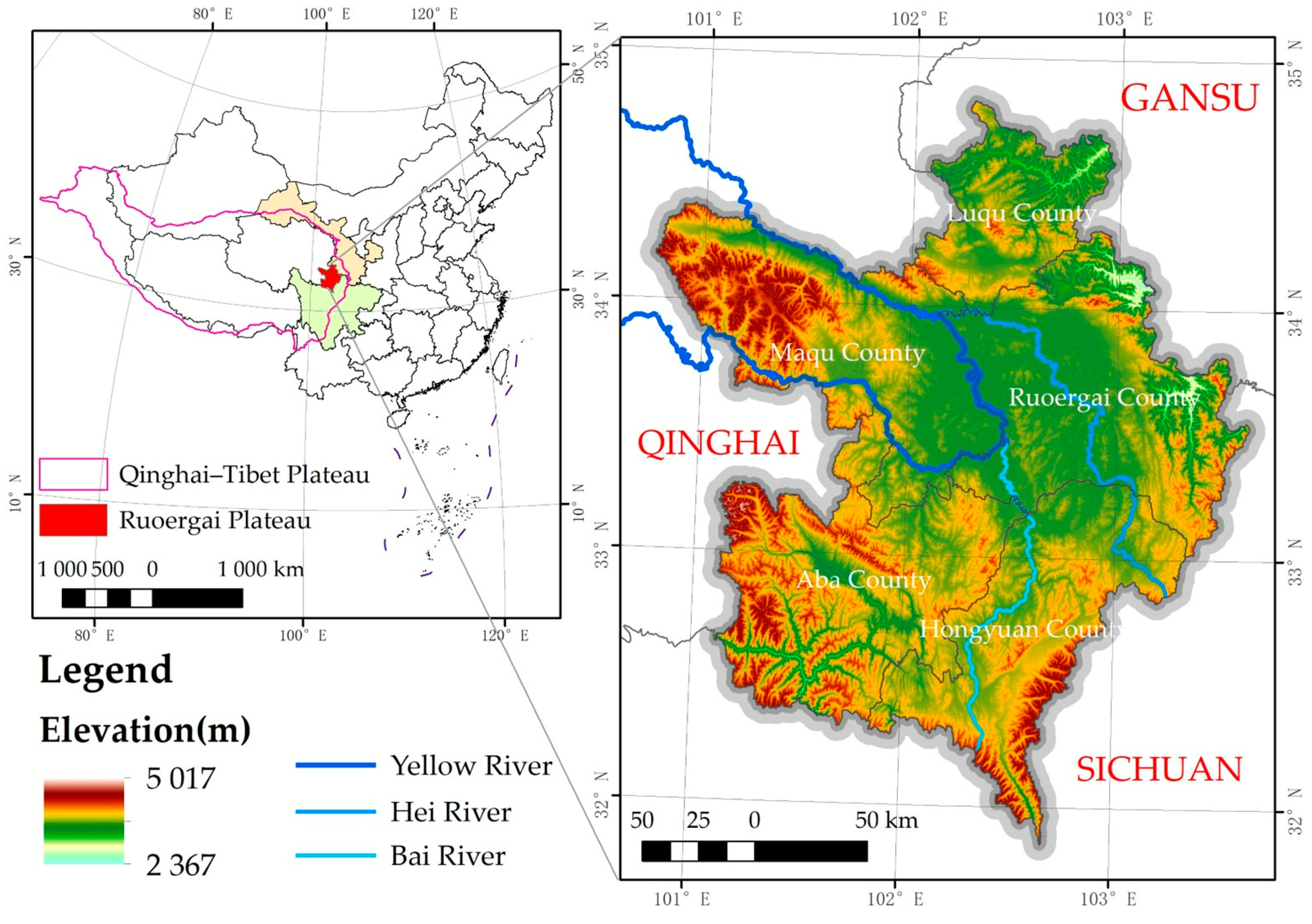
Figure 1. Location and extent of the study area in Ruoergai Plateau.
Land 12 01450 g001
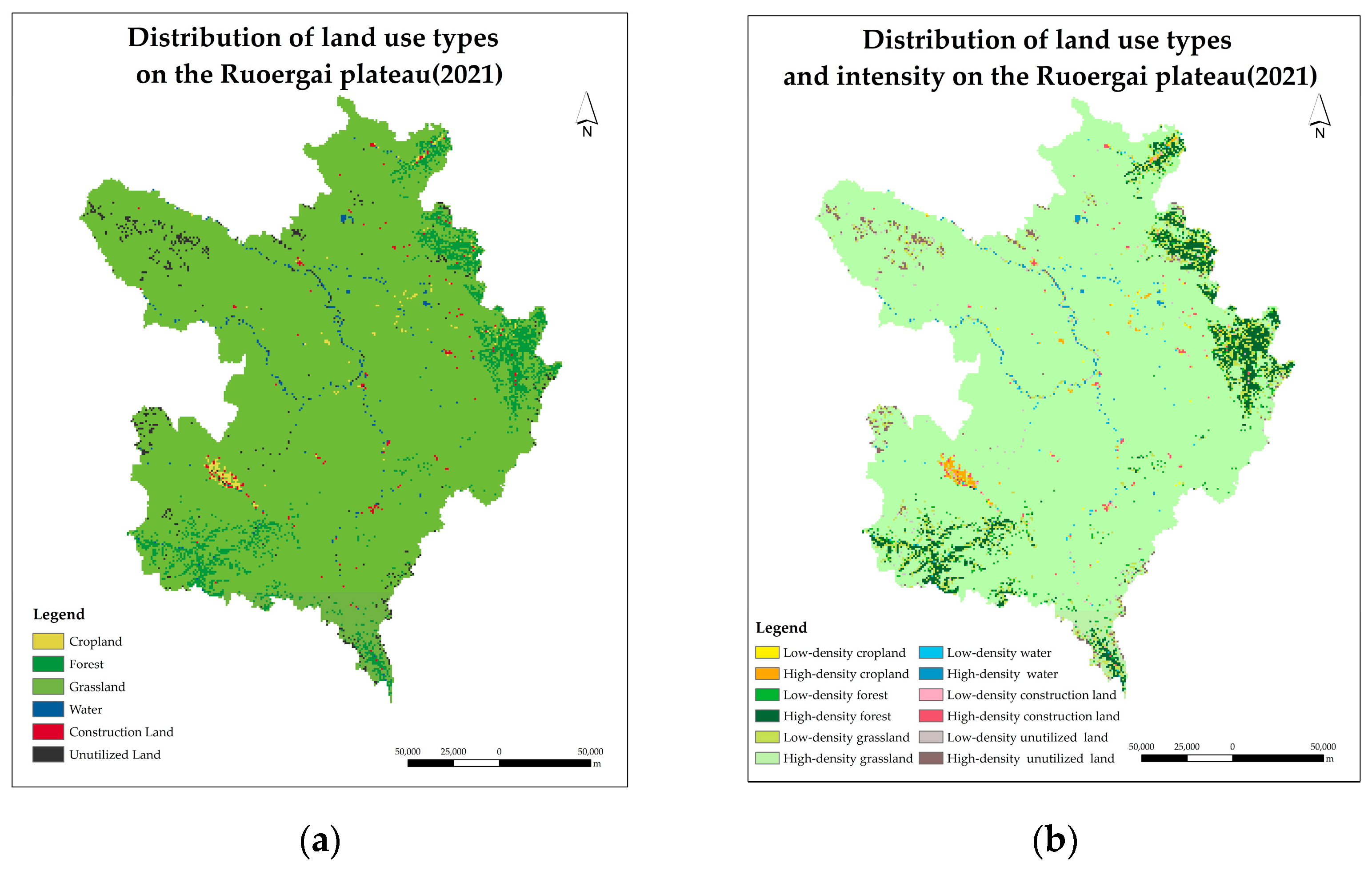
Figure 2. The land use/cover types and land use intensity data. (a) Six land use types distribution map of the Ruoergai Plateau. The results obtained are reliable because we have compared them with the land data from the Resource and Environment Science and Data Center [52] (b) Twelve land use intensity types of the Ruoergai Plateau. All the data have a 1 km resolution. The latter is divided by the natural breakpoint method based on the former.
Land 12 01450 g002
Figure 3. The production schematic diagram of compact cropland and scattered cropland.
Land 12 01450 g003
Figure 4. The driving factors.
Land 12 01450 g004
Figure 5. The overall framework of the integrated model (modified from reference [57]).
Land 12 01450 g005
Figure 6. The main work of this study.
Land 12 01450 g006
Figure 7. The core idea of calculating Boltzmann entropy for quantitative spatial raster data (modified from reference [60]).
Land 12 01450 g007
Figure 8. The Boltzmann entropy results were calculated by DEM on the Ruoergai Plateau. The higher the value, the greater the Botzmann entropy of the pixel, the greater the heterogeneity of space.
Land 12 01450 g008
Figure 9. Four sets of contrasting experiments were used to predict the 2021 land system based on 2017 data. (a) The model is integrated with MaxEnt and Boltzmann entropy. (b) The model is integrated with Boltzmann entropy. (c) The model is integrated with MaxEnt. (d) The original model.
Land 12 01450 g009
Figure 10. The confusion matrix between 2017 and 2021.
Land 12 01450 g010
Figure 11. Predicted results of land use types under 9 scenarios. Subfigure (ai) correspond to scenarios 1–9, respectively.
Land 12 01450 g011
Figure 12. Typical areas of land type and intensity distribution on the Ruoergai Plateau in 2021. The areas in the two red boxes are the selected typical areas.
Land 12 01450 g012
Figure 13. Local area 1 ((ai), in order, original 2021 scenario, scenarios 1–9).
Land 12 01450 g013
Figure 14. Local area 2 ((ai), in order, original 2021 scenario, scenarios 1–9).
Land 12 01450 g014
Figure 15. Summary of 2035 area for various land use types under different scenarios.
Land 12 01450 g015
Figure 16. Areas of (a) cropland; (b) forest; (c) grassland; (d) water; (e) construction; (f) unutilized land in 2035 under different simulation scenarios.
Land 12 01450 g016
Figure 17. Summary of the pixel-by-pixel transformations of the Ruoergai Plateau’s land systems from 2021 to 2035 in scenario 9. (i.e., if 126.1% GDP increase and 2.5% GEP increase become possible).
Land 12 01450 g017
Table 1. Names and sources of driving factors of land use change.
CategoryNameAbbreviationsData Sources/Links
Socio-economic driving factorsDistance from traffic roadstrafficCalculated using Open Street Map
(https://www.openstreetmap.org (accessed on 24 May 2023))
Gross Domestic ProductgdpGlobal 1 km × 1 km gridded revised real gross domestic product and electricity consumption during 1992–2019 based on calibrated nighttime light data [53]
Nightlight datanightlightEOG Nighttime Light
(Index of/nighttime_light/annual/v20 (mines.edu))
Population density datapopGoogle Earth Engine Datasets
(https://developers.google.com/earth-engine/datasets/catalog/WorldPop_GP_100m_pop (accessed on 24 May 2023))
Natural-environmental driving factorsDigital Elevation ModeldemResource and Environmental Science and Data Center
(https://www.resdc.cn/DOI/DOI.aspx?DOIID=123 (accessed on 24 May 2023))
SlopeslopeCalculated based on the DEM
Slope aspectaspect
Normalized Difference Vegetation IndexndviResource and Environmental Science and Data Center
(https://www.resdc.cn/data.aspx?DATAID=257 (accessed on 24 May 2023))
Net primary productivitynppGLASS product
(Index of/NPP/AVHRR/GLASS_NPP_005D_YEAR/2015 (umd.edu))
The proportion of silt in soilsoilsiltResource and Environmental Science and Data Center
(https://www.resdc.cn/data.aspx?DATAID=260 (accessed on 24 May 2023))
The proportion of clay in soilsoilclay
The proportion of sand in soilsoilsand
Cropland production potentialpcropDataset of cropland production potential in China, Resource and Environmental Science Data Center (http://www.resdc.cn/DOI (accessed on 24 May 2023)) [54]
Average annual precipitationPre1 km monthly temperature and precipitation dataset for China from 1901 to 2017 [55]
Average annual temperaturetmp
Soil organic matter contentorganicSoilGrids250m 2.0 (https://soilgrids.org/ (accessed on 24 May 2023))
Soil moisturesoilmoistureA fine-resolution soil moisture dataset for China in 2002~2018 [56]
Table 2. Accuracy evaluation results. The Kappa statistic results from two types of similarity: similarity of quantity and similarity of location. Here quantity refers to the total number of cells taken in by each category found in the legend (in other words: the histogram) and location refers to the spatial distribution of the different categories on the map. Kappa = KHisto → KLoc. KHisto only depends on the total number of cells taken in by each category, and KLoc strictly depends on the spatial distribution of the categories on the map. The Fraction correct statistic is calculated as the number of equal cells divided by the total number of cells.
Experimental SetupKappaFraction CorrectKLocationKHistogram
MaxEnt and Boltzmann entropy0.7730.9520.8140.950
Only Boltzmann entropy0.5800.9290.8880.654
Only MaxEnt0.7660.9510.8160.938
Original model0.6270.9370.9890.634
Table 3. Table of ecological service value equivalents per unit area of terrestrial ecosystems in China.
Ecological ServicesForestGrasslandCroplandWetlandWaterDesert
Gas Regulation3.500.800.501.800.000.00
Climate Regulation2.700.900.8917.100.460.00
Water Harvesting3.200.800.6015.5020.380.03
Soil Formation and Protection3.901.951.461.710.010.02
Waste Treatment1.311.311.6418.1818.180.01
Biodiversity Conservation3.261.090.712.502.490.34
Food Production0.100.301.000.300.100.01
Raw Materials2.600.050.100.070.010.00
Recreation and Culture1.280.040.015.554.340.01
Total21.857.246.9162.7145.970.42
Table 4. Area of Cropland for grain crops, grain price (in RMB per ton), economic value (in ten thousand RMB per square kilometer).
CountyGrain Production (t)Grain Area (km2)
Ruoergai5987.5622.45
Hongyuan205.261.30
Aba6388.1040.46
Magu12,488.1979.09
Luqu3070.0015.12
Total Area28,139.12158.42
Table 5. Economic and ecological efficiency coefficients for each land use type on the Ruoergai Plateau.
Land Use TypeCroplandForestGrasslandWaterConstruction LandUnutilized Land
Economic benefit
coefficient (RMB/km2)
1,814,700990091,300690024,061,6000
Ecological efficiency
coefficient (RMB/km2)
391,2881,237,286409,9753,077,02800
Table 6. GDP (generated from different land use types), area (km2), and Economic Benefit Coefficient (in ten thousand RMB per square kilometer).
Land Use TypeCroplandForestGrasslandWaterConstruction LandUnutilized Land
Corresponding IndustriesAgricultureForestryAnimal HusbandryFisheryOther IndustriesNone
Ruoergai3674.00358.00119,483.00180.0063,850.000.00
Hongyuan3371.14815.6485,137.740.0041,301.480.00
Aba6337.00259.0046,993.000.0059,665.000.00
Magu12,388.30506.3261,495.780.00147,009.600.00
Luqu8352.52341.3845,696.420.0094,883.430.00
Entire study area34,122.962280.34358,805.94180.00406,709.510.00
Area188231439,287262169530
Economic Benefit coefficient181.470.999.130.692406.160.00
Table 7. Area (km2), economic and ecological efficiency coefficients for each land use type taking into account land use intensity (RMB/km2).
Land TypeEconomic Benefit CoefficientEcological Efficiency CoefficientArea in 2021
Low-density Cropland326,70070,42958
High-density Cropland1,270,300273,900139
Low-density Forest1300160,843462
High-density Forest6100767,1001851
Low-density Grassland33,800151,6861571
High-density Grassland81,300364,87137,716
Low-density Water700307,70094
High-density Water38001,723,129166
Low-density Construction Land2,646,800054
High-density Construction Land12,993,3000115
Table 8. Scenarios setting for future land demand.
ScenariosGEP Growth (%)GDP Growth (%)
Scenario 10.25%12.60%
Scenario 21.25%12.60%
Scenario 32.50%12.60%
Scenario 40.25%63.00%
Scenario 51.25%63.00%
Scenario 62.50%63.00%
Scenario 70.25%126.10%
Scenario 81.25%126.10%
Scenario 92.50%126.10%
Table 9. The confusion matrix for the land system in 2017 (Map 1) and 2021 (Map 2).
Map 101234567891011Sum Map 1
Map 2
01140071510012041
168400147001310116
2003466216102001012530
30041167065141020001793
41015151041188257310897661692
53035601522537,06019171012866337,632
600002116717000299
700001221130095132
8000016003190047
90100010008000310
101000715318115319123
1100004588010014194640
Sum Map 2581394621851157137,716941665411517335144,634
Table 10. The conversion resistance for each land type.
Land Type Codes01234567891011
Conversion resistance0.270.720.650.930.700.990.680.860.660.980.220.57
Table 11. The transfer matrix for the land system in 2017 (Map 1) and 2021 (Map 2).
Land Type Codes01234567891011
0110011100110
1110011001110
2001111001011
3001111001000
4111111001111
5001011001111
6000011110001
7000011110011
8000000001100
9000000000100
10100011111111
11000011010011
Table 12. The occupancy area for the nine scenarios (km2).
ScenariosOrigin123456789
Land Types
0584319122030000
11391291631748095103101101101
246236924466100000
31851178118271900159117321790167116671657
4157112659725843504218151414
537,71638,18838,54639,02139,19939,37039,25938,86138,84138,804
69472584018139999
7166145153185127139183163169181
854163181188688679718123112451279
9115139132128227228220250255256
10173130129126123123124123123123
11351326326326326326326326326326
Disclaimer/Publisher’s Note: The statements, opinions and data contained in all publications are solely those of the individual author(s) and contributor(s) and not of MDPI and/or the editor(s). MDPI and/or the editor(s) disclaim responsibility for any injury to people or property resulting from any ideas, methods, instructions or products referred to in the content.