Study on the Spatiotemporal Evolution of the “Contraction–Expansion” Change of the Boundary Area between Two Green Belts in Beijing Based on a Multi-Index System

Abstract

In serving as a pivotal strategy for curbing urban sprawl, large-scale urban green belts, being a significant constituent of the urban green space, have been ubiquitously employed in the scheming and fabrication of green space systems in global megacities. Nevertheless, the disregard for research into the independent alteration mechanism of urban green space, coupled with the reactive approach of planning and construction and the singularity of quantitative indices, has engendered challenges in the creation of urban green belts. This paper presents an investigation into the juncture zone of two green belts in Beijing as a case study, erecting a “contraction–expansion” flux model of its green space and gauging the transformational traits of the green space in light of its spatial–temporal evolution with regards to its quantity, space, and connectivity among others. Findings reveal that between 2005 and 2012, the green space in Beijing underwent an approximately 20% alteration, with the green belt intersection zone’s green space area experiencing a dual trajectory shift of “expansion-contraction”. This shift was primarily characterized by expansion before 2015 and contraction from 2015 onwards. Concerning spatial attributes, patterns of expansion and aggregation were discernible in scattered distribution, whereas contraction and aggregation were evident in mass and spaced distribution. Spatial stability was influenced by the change model, marked by a shift in the center of gravity from a “north-south-east” orientation to a “northwest-southeast” direction. At the connectivity stratum, noticeable variations were witnessed in both the overall and local connectivity levels pre- and post-2015. Regarding individual connectivity, three vital nodes of stable linear connectivity were identified, playing a decisive role in defining the dispersion of crucial corridors within the area of study.

1. Introduction

Urban green belts globally serve as an instrumental mechanism to regulate urban expansion, an assertion supported by an abundance of literature [1,2,3,4]. In spite of ceaseless critiques pertaining to their effectiveness and the challenges of actual implementation [5,6,7], it remains a salient point that in numerous developing and emerging nations, the crux of urban development conflict resides in the inconsistent scales of construction and irreversible damage imparted on urban ecosystems due to construction land expansion under the influence of population growth [8,9,10,11,12,13,14,15]. The reactive nature of urban green space transformation mechanisms is particularly noteworthy. Beijing, China’s capital and one of its megacities, experiences urban sprawl as its foremost developmental issue. Since the 1950s, Beijing has advocated for the application of urban green belts as a means to regulate urban sprawl, yet the management has proven to be relatively reactive [4]. In essence, the feasibility of green space development hinges on the level of control exerted over the construction land upon which it is constructed. It is against this backdrop that Beijing’s inaugural green belt deviated from its original construction objectives [16,17,18]. Moreover, this “green space reactivity” is observable not only in government operations but also in urban space change studies. To elaborate, we are yet to establish an independent mechanism pattern and research perspective of green space within the realm of urban space, thereby failing to reflect the equity, autonomy, and proactive nature of different land-use types, particularly green spaces, in terms of their value bearing and supply functions.

The issue of reactivity also permeates the planning and construction of urban green spaces. The demarcations of administrative boundaries in China emanate from a national hierarchical management system wherein planning targets and developmental resources are allocated through a rigid, downward spatial administration system [19,20,21]. As such, this boundary management system prevails not solely between provinces and cities but also within smaller scale entities such as urban districts and ecological land areas. While this boundary system facilitates clear ownership from a planning control standpoint, offering convenience and standardization for multi-level planning implementation, it morphs into a restriction rather than a facilitator when distinct urban sectors share common economic, cultural, and ecological objectives. Recently, the Chinese government has acknowledged this predicament and proposed a plethora of development strategies targeting regional integration, albeit with a tendency to overlook eco-regional integration issues. The two belts, marked by their unique construction eras, backgrounds, scales, and objectives, have distinctly delineated planning boundaries. These definitive planning boundaries yield the effect of severing urban construction, and the multifaceted landscape structures of greenways, green networks, and green belts within the regions are subject to administrative jurisdiction. This often leads to outcomes that contradict original planning goals. Shifting the focus to their interface characteristics rather than their linear properties holds significant potential for mitigating this issue.

The uniqueness of urban green space indicator evaluation. A significant proportion of prior research primarily revolves around the fragmentation of green space [22,23], the landscape pattern of green space [24,25,26], and changes in green space vegetation cover [27,28], thereby exhibiting a lack of diversity in the analysis of indicators.

There exists a critical need to establish an autonomous mechanism for green land-use changes, concentrate on green regions segmented by administrative boundaries, integrate ecological gray zones, and holistically consider the value of green lands. This study endeavors to contemplate the planning and construction of the entire green space from a macroscopic vantage point, inclusive of the first and second green belts. By using the boundary area in Beijing as the research subject, this article clarifies the specific extent and conceptual definition of the area and proposes the fundamental connotation of the “contraction–expansion” mechanism of green space. Subsequently, diverse evaluation indicators are constructed from three perspectives: quantity, space, and connectivity. Furthermore, the study enhances the content and description subjects of the indicators, scrutinizes the land-use change pattern at the boundary between Beijing’s two green belts from 2005 to 2020, and provides a scientific basis for the planning and construction of green space in Beijing.

2. Concept of “Contraction–Expansion” Evolution

The idea of spatial evolutionary types traces its roots back to patch evolutionary concepts, a terminology utilized extensively within the domain of forestry research to depict the metamorphosis of minor patch topologies and structures. Utilizing this as a foundation, Qiong Wang [29] propelled this classification scheme from forest science into urban greenspace studies, thereby delineating the evolutionary types of urban green space patches within the broader discourse of their evolution. An enlargement in the extent of urban green space patches is conceptualized as an “expansion” evolutionary type, while a reduction is encapsulated within the “contraction” evolutionary type, aimed at depicting the existing evolutionary states throughout urban green space evolution. Drawing upon prior research, this paper defines the “contraction–expansion” evolutionary type of green spaces as the morphing of urban green space patches’ land-use types spurred by urbanization, engendering the dynamic phenomena of geographical and quantitative changes in the form of increasing or decreasing areas. Previous [20,22,30] has devoted considerable attention to the contraction of urban green space, delving into the fragmentation of such spaces, the causative agents behind their shrinkage, and other ecological issues resulting from this reduction. The strength of these studies resides in their ability to provide an accurate depiction of the dynamic relationship between urban sprawl and green space diminution, thus deciphering the patterns. Nonetheless, they suffer from a certain narrowness of perspective, failing to comprehend the dynamism inherent in urban green space changes fully and consequently neglecting the vital role of urban policies. Urban green space transformations are often multifaceted and comprehensive, hence concentrating on their dynamism allows for a more robust understanding of the urban green space’s evolutionary mechanisms and a holistic evaluation of the urbanization process’s impact on these spaces. This understanding is instrumental for the implementation of more effective future urban planning initiatives.

This paper scrutinizes the “contraction–expansion” shift pattern via three distinct approaches: first, by cataloging the specific instances of the “contraction–expansion” transition pattern in the context of urban development and planning stipulations; second, by simulating the “contraction–expansion” state of flux through expansion; third, by narrating and explicating the current land-use alteration patterns.

3. Data Source and Processing

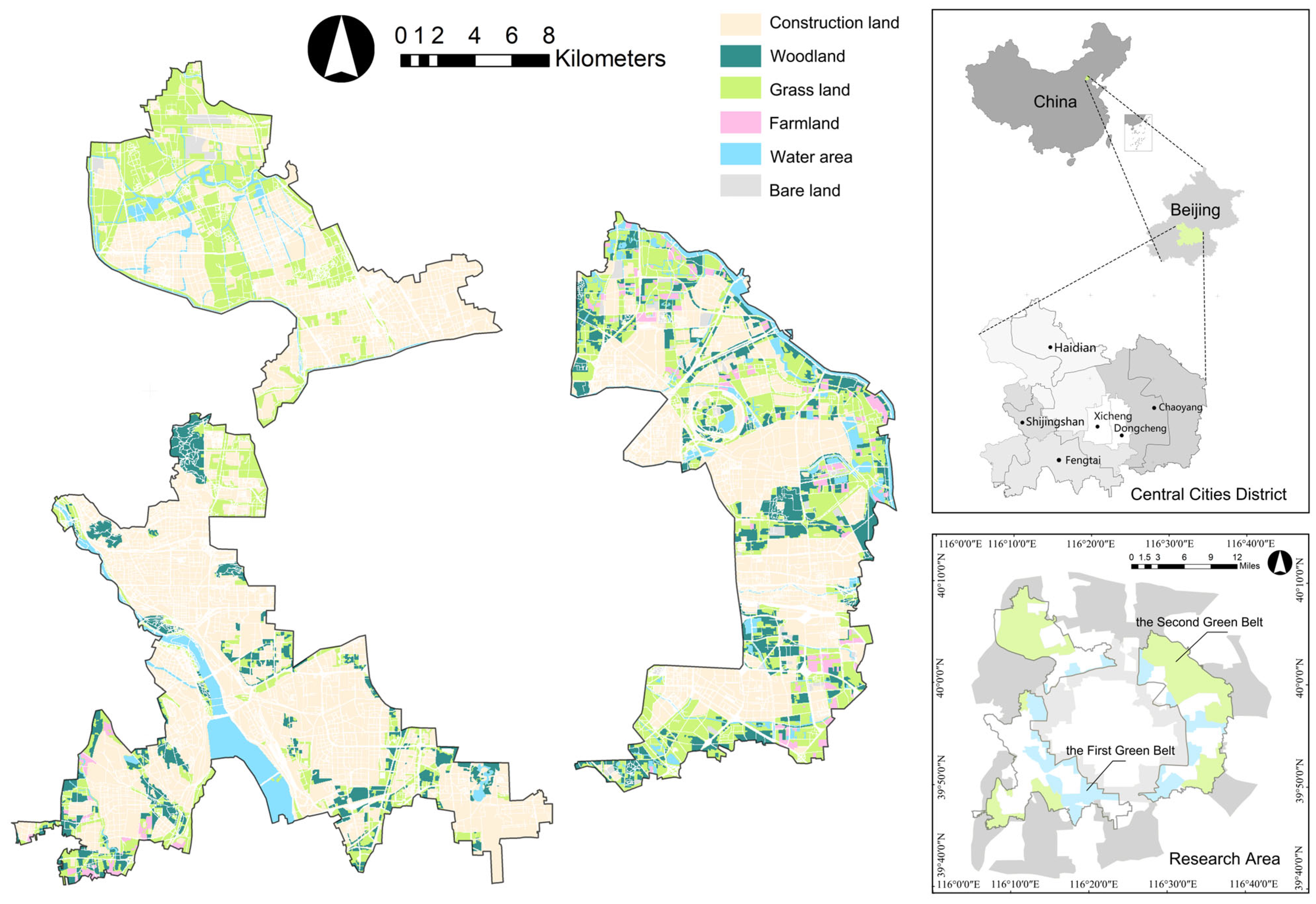
The dataset employed in this study encompasses 10 m land-use data for the years 2005, 2015, and 2020. The data for 2005 and 2015 were procured from the project team, and their accuracy was verified by ENVI 5.4 software using Overall Accuracy (OA) and kappa coefficient based on the confusion matrix [31]. The findings denote that the 2005 and 2015 data for Beijing harbor an OA of 92.4719% and a kappa coefficient of 0.9045, thus substantiating their reliability. The 2020 land-use data were sourced from the European Space Agency’s 10 m global land-use data repository (https://viewer.esa-worldcover.org/worldcover, accessed on 12 April 2023).

4. Research Area

The study area is demarcated between the first and second green belts nestled within Beijing’s central urban expanse (excluding non-plain zones). As delineated in Figure 1, the total area spans 696.75 km², with coordinates of 39°45′–40°9′ north latitude and 116°4′–116°38′ east longitude. The average elevation is 42 m, which constitutes approximately 4.25% of Beijing’s total extent. The extant green space area measures 128.73 km², whereas the planned green space is pegged at 230.38 km². The entire region encompasses four administrative districts, Haidian, Chaoyang, Fengtai, and Shijingshan, rendering a central surrounding layout. According to the “Beijing Central Urban Area Municipal-level Greenway System Plan”, the inner boundary delineates the urban park ring in the city center (the first green belt), and the outer boundary denotes the threshold between the urban near suburbs and far suburbs (inside the second green belt).

5. Construction of a Multidimensional Indicator System

Ecological planning typically necessitates analysis and interpretation from multifarious perspectives. As an increasing number of indicators are amalgamated into the quantitative analysis of ecological planning, research should remain faithful to the overarching direction of multi-objective planning, consequently forming a multifaceted quantitative system. It is incumbent upon us to elucidate in a scientific and lucid manner the challenges encountered in the urban ecological status amid the urban development process. This study will scrutinize the land-use change characteristics of the green ecotone zone from three vantage points: quantity change, spatial characteristics, and connectivity, as Figure 2 shown.

5.1. Change in Quantity Level—Area Change under “Contraction–Expansion” Mode

Quantity change serves as a metric to evaluate the characteristics of urban land-use area changes from a statistical viewpoint. A deductive analysis of land-use alterations among different land categories in the green belt ecotone zone, from the perspective of temporal evolution, can offer a more precise understanding and analysis of shifts in urban green space areas. Simultaneously, aided by the Land Use Patterns Tupu method, a detailed deconstruction of the “map unit” within the green belt ecotone zone can be achieved at the micro-scale level. This Tupu method, initially advocated for by Chen Shupeng [32], offers an enhanced quantification of the variations across diverse land types and can be effectively dovetailed with the “contraction–expansion” transition pattern to elucidate its mechanism and characteristics. Despite demonstrating certain advantages, its application in land-use change research has been relatively sparse.

Area fluctuations within the “contraction–expansion” paradigm primarily encompass area changes under contraction mode, stable mode, expansion mode, and subordinate mode changes within each category. All three computations leverage the graph method and are subsequently classified to calculate their area values. The formula is as follows:

$$\mathrm{P}=\sum _{\mathrm{E}=1}^{\mathrm{N}}{\mathrm{Q}}_{\mathrm{E}}{10}^{\mathrm{N}-\mathrm{E}}(\mathrm{N}\ge 1)$$

where P signifies the land use across varying continuums of expansion intensities within the studied region relative to the attribute values of the new mapping grid unit; N denotes the count of consecutive periods investigated; E corresponds to the chronological sequence number; and ${\mathrm{Q}}_E$symbolizes the attribute value of land-use grid for the Eth period within the examined area. This study amalgamated three periods of land-use change pattern mapping, aligning the encoding order of mapping units with the chronological series. In other words, the initial encoding signifies the land type in 2005, the subsequent encoding represents the land type in 2015, and the final encoding corresponds to the land type in 2020.

5.2. Space Characteristics Level—Morphological Features and Spatial Distribution

The morphology and configuration of urban spaces can, to some extent, mirror the state and pattern of the urban ecological system, thereby making it an essential factor when applying landscape ecology to urban spatial research. The examination of morphological characteristics and spatial distribution of green corridors is primarily twofold: spatial aggregation and spatial stability. The spatial aggregation index is derived by translating the land-use map equation into a geographic spatial graph through ArcGIS software and, subsequently, conducting a qualitative analysis of its aggregation traits. Spatial stability, on the other hand, is examined via the Spatial Structure Stability Index (SSSI) [33]. The SSSI is computed based on the Spatial Structure Conflict Index (SCCI), which provides a positive representation of the green space characteristics. The formula is:

$$\mathrm{S}\mathrm{S}\mathrm{S}\mathrm{I}=1-\mathrm{S}\mathrm{C}\mathrm{C}\mathrm{I}$$

The formula for SCCI is:

$$\mathrm{S}\mathrm{C}\mathrm{C}\mathrm{I}=\mathrm{C}\mathrm{I}+\mathrm{F}\mathrm{I}-\mathrm{S}\mathrm{I}$$

where CI refers to conflict index, FI refers to fragility index, and SI refers to stability index.

Therefore, the expression formula for SSSI is:

$$\mathrm{S}\mathrm{S}\mathrm{S}\mathrm{I}=1-\mathrm{C}\mathrm{I}-\mathrm{F}\mathrm{I}+\mathrm{S}\mathrm{I}$$

Using the Area Weighted Average Patch Fractal Dimension (AWMPFD), the complexity of landscape patterns caused by natural or anthropogenic influences [34], we represent CI with the formula:

$$\mathrm{A}\mathrm{W}\mathrm{M}\mathrm{P}\mathrm{F}\mathrm{D}=\sum _{\mathrm{i}=1}^{\mathrm{m}}\sum _{\mathrm{j}=1}^{\mathrm{n}}\left[\frac{2\mathrm{l}\mathrm{n}\left(0.25{\mathrm{P}}_{\mathrm{i}\mathrm{j}}\right)}{\ln \left({\mathrm{a}}_{\mathrm{i}\mathrm{j}}\right)}\left(\frac{{\mathrm{a}}_{\mathrm{i}\mathrm{j}}}{\mathrm{A}}\right)\right]$$

where ${\mathrm{P}}_{\mathrm{i}\mathrm{j}}$and ${\mathrm{a}}_{\mathrm{i}\mathrm{j}}$ denote the area and perimeter of patches, respectively; A signifies the area of each spatial unit at the landscape level; m is the aggregate number of patches in the study area; and n corresponds to the count of spatial types. The results are subsequently normalized to a range between 0 and 1. The order of landscape vulnerability from robust to feeble, as suggested by the Fragility Index (FI), is as follows: 6 (construction land), 5 (unused land), 4 (farming land), 3 (forest land), 2 (grassland), and 1 (water body). After assigning values to each category of land use employing ARCGIS 10.2 software, the final outcome is normalized within the range (0, 1]. The formula for the Stability Index (SI) is:

$$\mathrm{S}\mathrm{I}=1-\mathrm{P}\mathrm{D}$$

The term PD embodies patch density, where escalated values signal a heightened level of fragmentation and diminished stability. The formula is expressed as:

$$\mathrm{P}\mathrm{D}=\frac{{\mathrm{n}}_{\mathrm{i}}}{\mathrm{A}}$$

where ${\mathrm{n}}_{\mathrm{i}}$ represents the count of patches in the i-th category and A denotes the total landscape area or patches. The resultant SI is normalized to the range (0, 1].

For a superior measure of the spatial stability of the interwoven zone of the circular green belt, ArcGIS will be deployed for visual analysis from two standpoints: overall stability, and stability values above the median value, referred to as Above-middle-level Green Spaces (AGS). In conjunction with the Standard Deviation Ellipse (SDE) analytical method, ARCGIS 10.2 software will be used to investigate the distribution center, direction, and shape of stable or highly stable areas. SDE mirrors the data distribution by gauging the mean and standard deviation using an elliptical representation. It can unravel the multifaceted spatial positioning traits of geographic elements, encompassing centrality, directionality, and spatial morphology. The calculation formula for SDE primarily comprises:

$${\mathrm{C}}_{\mathrm{S}\mathrm{D}\mathrm{E}}=\left(\begin{array}{cc}\mathrm{v}\mathrm{a}\mathrm{r}\left(\mathrm{x}\right)& \mathrm{c}\mathrm{o}\mathrm{v}(\mathrm{x},\mathrm{y})\\ \mathrm{c}\mathrm{o}\mathrm{v}(\mathrm{x},\mathrm{y})& \mathrm{v}\mathrm{a}\mathrm{r}\left(\mathrm{y}\right)\end{array}\right)=\frac{1}{\mathrm{n}}\left(\begin{array}{cc}{\displaystyle \sum _{\mathrm{i}=1}^{\mathrm{n}}}{\tilde{\mathrm{x}}}_{\mathrm{i}}^2& {\displaystyle \sum _{\mathrm{i}=1}^{\mathrm{n}}}{\tilde{\mathrm{x}}}_{\mathrm{i}}{\tilde{\mathrm{y}}}_{\mathrm{i}}\\ {\displaystyle \sum _{\mathrm{i}=1}^{\mathrm{n}}}{\tilde{\mathrm{x}}}_{\mathrm{i}}{\tilde{\mathrm{y}}}_{\mathrm{i}}& {\displaystyle \sum _{\mathrm{i}=1}^{\mathrm{n}}}{\tilde{\mathrm{y}}}_{\mathrm{i}}^2\end{array}\right)$$

$$\mathrm{v}\mathrm{a}\mathrm{r}(\mathrm{x})=\frac{1}{\mathrm{n}}\sum _{\mathrm{i}=1}^{\mathrm{n}}{\left({\mathrm{x}}_{\mathrm{i}}-\overline{\mathrm{x}}\right)}^2=\frac{1}{\mathrm{n}}\sum _{\mathrm{i}=1}^{\mathrm{n}}{\tilde{\mathrm{x}}}_{\mathrm{i}}^2$$

$$\mathrm{c}\mathrm{o}\mathrm{v}(\mathrm{x},\mathrm{y})=\frac{1}{\mathrm{n}}\sum _{\mathrm{i}=1}^{\mathrm{n}}\left({\mathrm{x}}_{\mathrm{i}}-\overline{\mathrm{x}}\right)\left({\mathrm{y}}_{\mathrm{i}}-\overline{\mathrm{y}}\right)=\frac{1}{\mathrm{n}}\sum _{\mathrm{i}=1}^{\mathrm{n}}{\tilde{\mathrm{x}}}_{\mathrm{i}}{\tilde{\mathrm{y}}}_{\mathrm{i}}$$

$$\mathrm{v}\mathrm{a}\mathrm{r}(\mathrm{y})=\frac{1}{\mathrm{n}}\sum _{\mathrm{i}=1}^{\mathrm{n}}{\left({\mathrm{y}}_{\mathrm{i}}-\overline{\mathrm{y}}\right)}^2=\frac{1}{\mathrm{n}}\sum _{\mathrm{i}=1}^{\mathrm{n}}{\tilde{\mathrm{y}}}_{\mathrm{i}}^2$$

where x and y are the coordinates of the i-th element, $\{\overline{\mathrm{x}}, \overline{\mathrm{y}}\}$ $\{\overline{x},\overline{y}$} represents the average center of the elements, and n is the total number of elements.

The sample covariance matrix is decomposed into standard form such that the matrix can be represented by eigenvalues and eigenvectors. Thus, the standard deviation of the x and y axes is:

$${\mathsf{\sigma }}_{\mathrm{1,2}}={\left(\frac{(\sum _{i=1}^n{{\tilde{x}}_i}^2+\sum _{i=1}^n{{\tilde{y}}_i}^2)\pm \sqrt{(\sum _{i=1}^n{{\tilde{x}}_i}^2-\sum _{i=1}^n{{\tilde{y}}_i}^2{)}^2+4{\left(\sum _{i=1}^n{\tilde{x}}_i{\tilde{y}}_i\right)}^2}}{2n}\right)}^{1/2}$$

5.3. Connectivity Level—Global and Local Level of Connectivity

Landscape connectivity analysis was conducted using Graphab 2.6 software (https://sourcesup.renater.fr/www/graphab/en/home.html, accessed on 11 June 2023), a graph theory-based tool for landscape connectivity metric computations. Graphab identifies corresponding land-use types as ecological source patches, predicated on the habitat preferences of indicator species [35]. Amphibians, particularly toads, which are widely distributed in Beijing and highly sensitive to ecological degradation, serve as quintessential indicator species within urban ecosystems, offering prompt feedback concerning environmental modifications [36]. Habitat fragmentation and loss over the past decade have instigated a consistent decrease in their populations. Consequently, they were selected as indicator species for green belt connectivity calculations in this study. Construction land, due to its strong human disturbance, is perceived as detrimental to survival, hence is allocated a value of 100. Conversely, the remaining beneficial land types are assigned a value of 10. A distance threshold of 1500 m was established for this study [37].

Connectivity capacity is a quantitative metric that encapsulates the ecological interactions between different patches, encompassing both global and local connectivity. The Connectivity Probability (PC) is utilized to gauge both overall and local connectivity, supplemented by additional analysis conducted using the maximum and average connectivity unit capacities (SLC and MSC). The Connectivity Probability (PC) serves as an ecological connectivity index at the landscape scale, delineated as “the probability that two points, randomly situated within the landscape, fall into each other’s accessible habitat areas”. In this study, it is employed to represent the connectivity amongst various green spaces, and the formula is as follows:

$$\mathrm{P}\mathrm{C}=\frac{{\sum }_{\mathrm{i}-1}^{\mathrm{n}}{\sum }_{\mathrm{j}-1}^{\mathrm{n}}{\mathsf{\alpha }}_{\mathrm{i}}{\mathsf{\alpha }}_{\mathrm{j}}{\mathrm{P}}_{\mathrm{i}\mathrm{j}}^{\mathrm{n}}}{{{\mathrm{A}}_{\mathrm{L}}}^2}$$

Let ${\mathsf{\alpha }}_{\mathrm{i}}$ and ${\mathsf{\alpha }}_{\mathrm{j}}$ denote the green space areas of patch i and patch j, respectively. We employ n to indicate the total number of such green spaces, while ${\mathrm{A}}_{\mathrm{L}}$ stands for the aggregate land area. ${\mathrm{P}}_{\mathrm{i}\mathrm{j}}^{\mathrm{n}}$ encapsulates the maximum patch rate traversing either directly or indirectly between patch I and patch j.

The Fraction of Delta Probability of Connectivity (dPC) is determined by computing the percentile decline of PC, considering both the existence and subsequent absence of a particular plaque. The formula for such calculation is as follows:

$$\mathrm{d}\mathrm{P}\mathrm{C}=\frac{(\mathrm{P}\mathrm{C}-{\mathrm{P}\mathrm{C}}_{\mathrm{i}}^{\prime })}{\mathrm{P}\mathrm{C}}$$

The Size of the Largest Component (SLC) signifies the capacity of the most extensive, mutually connected patch cluster within the ecological network. A higher SLC value corresponds to a heightened dominance and concentration of the associated patch clusters, bolstering the resilience of the core ecological source patch against interference. This, in turn, implies a superior level of global connectivity. The computational formula is provided below:

$$\mathrm{S}\mathrm{L}\mathrm{C}=\max \left\{\mathrm{a}{\mathrm{c}}_{\mathrm{k}}\right\}$$

In the formula, ${\mathrm{a}\mathrm{c}}_{\mathrm{k}}$ denotes the capacity of landscape connectivity k, which is an aggregate capacity of the patches constituting k.

Mean Size of the Components (MSC) symbolizes the average capacity of a mutually connected patch cluster in the ecological network. An increased MSC value advocates for an enhanced intra-connectivity within a single connected unit, thereby strengthening the unit’s ability to counter ecological threats and elevating the ecological stability. The mathematical equation for such calculation is provided below:

$$\mathrm{M}\mathrm{S}\mathrm{C}=\frac{1}{\mathrm{n}\mathrm{c}}\sum _{\mathrm{k}=1}^{\mathrm{n}\mathrm{c}}\mathrm{a}{\mathrm{c}}_{\mathrm{k}}$$

In the equation, $\mathrm{n}\mathrm{c}$ represents the number of landscape connectivity components, while $\mathrm{a}{\mathrm{c}}_{\mathrm{k}}$ symbolizes the capacity of landscape connectivity component k, calculated as the total of patch capacities forming k.

6. Results

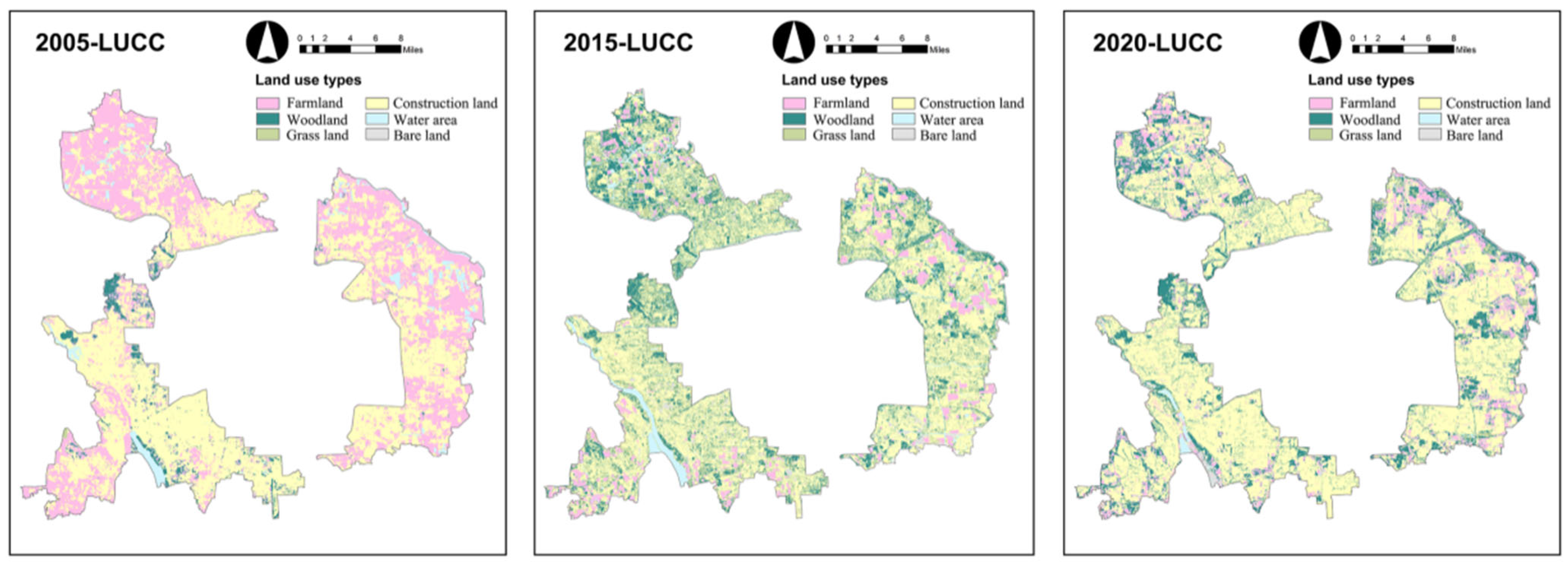
6.1. Analysis of Green Space Land-Use Area from 2005–2020

Figure 3 delineates the dynamics of land-use changes within the green belt interlacing zone spanning from 2005 to 2020. This figure illustrates the nuanced variations of land-use trends over the course of fifteen years, with the year 2015 acting as a watershed. Prior to 2015, land-use changes were typified by the notable conversion of green spaces—composed of forests, grasslands, and water bodies—into cultivated land, signifying a period characterized by rapid urban ecological construction. Following 2015, the green belt witnessed a surge in urban economic construction, with the expansion of construction land as its primary characteristic.

Table 1. Land-use changes of the boundary between two green belts from 2005 to 2020.

Land-Use Type	Farm Land	Forest Land	Grass Land	Construction Land	Water	Vacant Land
	/km2	/km2	/km2	/km2	/km2	/km2
2005	264.43	18.96	0.49	383.48	23.21	0.14
%	38.28	2.75	0.07	55.52	3.36	0.02
2015	56.51	110.19	122.52	348.72	37.27	15.50
%	8.18	15.95	17.74	50.49	5.40	2.24
2020	77.72	107.85	13.21	456.77	7.67	27.28
%	11.25	15.61	1.91	66.13	1.11	11.25

presents that, notwithstanding the fluctuations in land-use attributes during different periods within the green belt interlacing zone, the land-use pattern remains predominantly dictated by the area of construction land, accounting for 55.52%, 50.49%, and 66.13% from 2005 to 2020, respectively. Predicated on this pattern, it can be inferred that the “contraction–expansion” mechanism of the large green spaces is shaped around the evolution of non-green spaces, principally occupied by construction land, and the alteration of diverse land-use categories within green spaces.

During the decade of 2005 to 2015, a 5.03% decrease compared to 2005 was observed. Notably, among the various green space classifications, forest area (110.19 km²) and grassland area (122.52 km²) underwent a considerable enlargement. This expansion of forest and grassland spaces was positively influenced by the Million Mu Afforestation Project in Beijing’s plains and environmental protection and ecological construction initiatives during the Eleventh Five-Year Plan period.

In contrast, between 2015 and 2020, there was a substantial surge in the construction land area, presenting a stark difference in comparison to the preceding decade. The proportion of total construction land area escalated from 50.49% to 66.13%. In respect to green space alterations, the forest land area in 2020 (107.85 km²) remained relatively static compared to that in 2015; conversely, the grassland and water areas witnessed a steep “contraction”, with their proportions dwindling from 17.74% to 1.91% and from 5.40% to 1.11%, respectively. These findings suggest that vertically simple green spaces are more vulnerable to the effects of rigid land use.

6.2. Analysis of the Multiple Index System of Green Spaces from 2005 to 2020

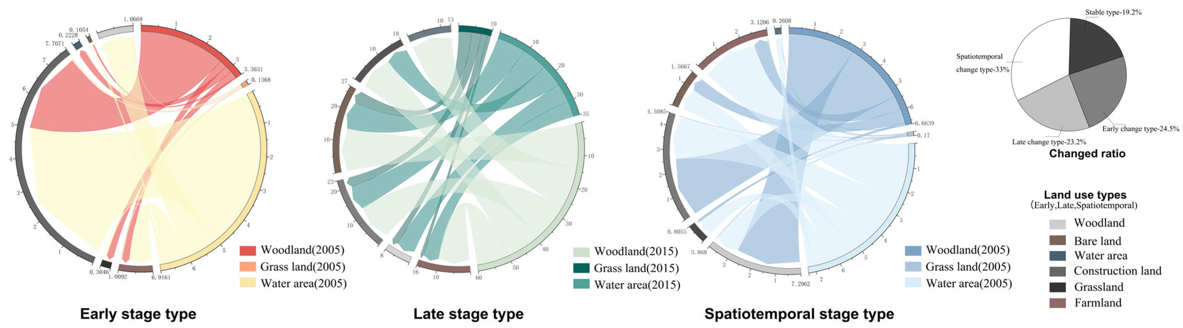
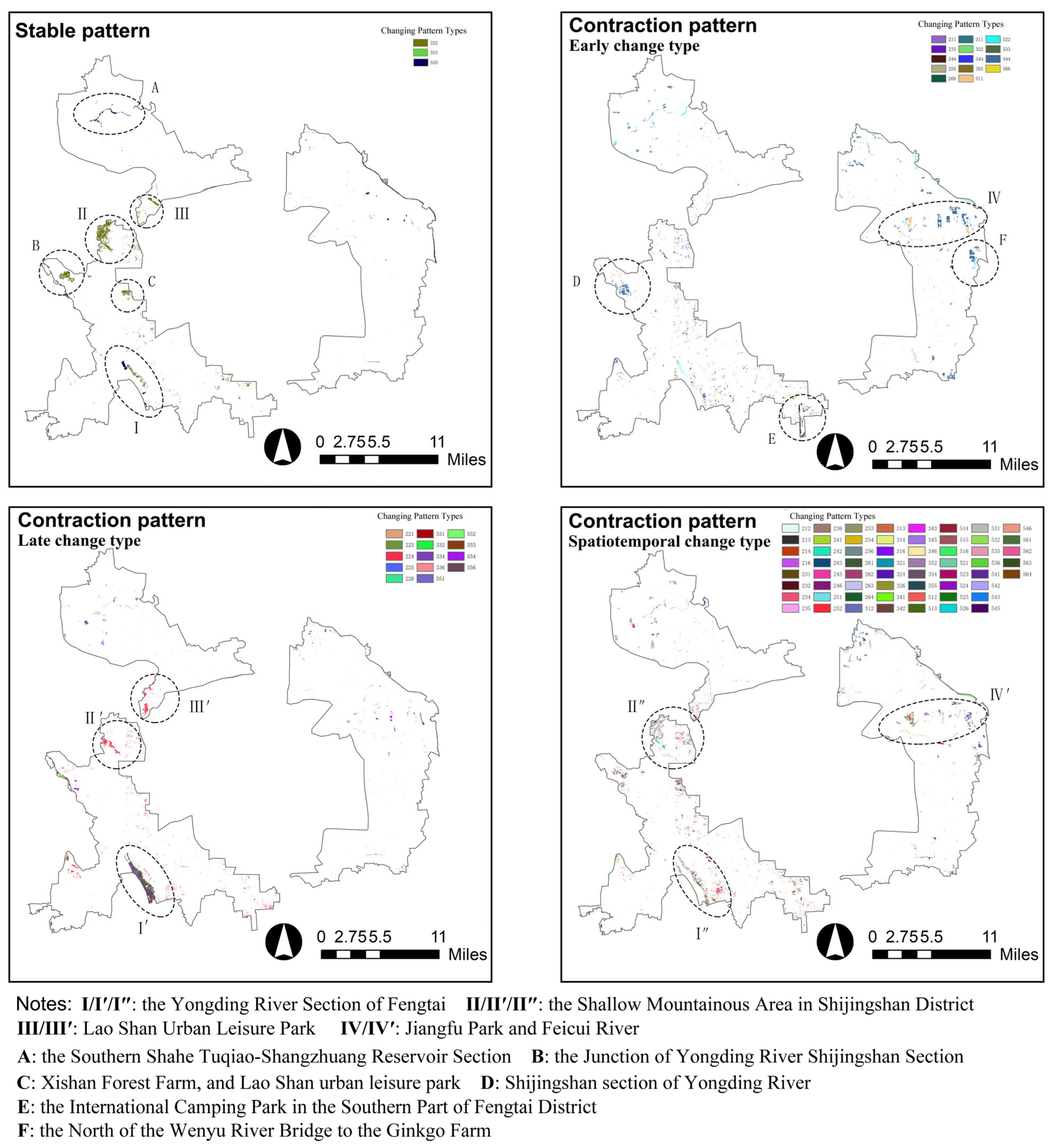
6.2.1. Analysis of the Area Changes in the “Contraction–Expansion” Pattern of Green Space

The dynamism of green space’s internal structure adjustments is not only a function of spatial self-regulation but also of the expansion impetus brought forth by non-green space conversion. Moreover, not all green space types undergo alterations or unidirectional transformations. Certain categories of green land maintain stability, while some green spaces revert to their original state after undergoing a non-green space conversion phase. Given the complexity of these scenarios, this study seeks to comprehend the mechanisms underlying the “contraction–expansion” transition pattern across different temporal scales and transformation frequencies. Three fundamental pattern types—stable, contraction, and expansion—have been identified, and their respective characteristics and subtypes of changes are systematically outlined.

Stable and Contraction Patterns of Green Space

The stable pattern of green space refers to the pattern that retains its original land-use type without any alterations between 2005 and 2020. The contraction pattern pertains to the green space that has been transformed into different land-use types. Considering the current landscape, the top 15 contraction patterns, characterized by significant area variations, are subdivided into 3 subtypes: 1. The early transformation type, referring to green spaces that underwent land-use change exclusively between 2005 and 2015. 2. The late transformation type, referring to those that underwent land-use change solely between 2015 and 2020. 3. The spatiotemporal transformation type, characterizing green spaces that experienced land-use changes during both the 2005–2015 and 2015–2020 periods.

As shown in

Table 2. The land-use change of green spaces in the boundary area between two green belts from 2005 to 2020.

Changing Pattern		Time	Changing Time	Pattern-Change Illustration	Changed Area/km2	Changed Ratio/%
Stable pattern		2005–2020	0	a-a-a	8.17	19.24
Contraction pattern	Early change type	2005–2015	1	a-b-b	10.42	24.54
	Late change type	2015–2020	1	a-a-b	9.84	23.17
	Spatiotemporal change type	2005–2020	2	a-b-c/a-b-a	14.03	33.04

, among these four transformation patterns, the spatiotemporal transformation type constitutes the highest proportion (33.04%), whereas the spatiotemporal stability type carries the lowest proportion (19.24%). These findings suggest a limited stability of green space lands from 2005 to 2020, highlighting a highly dynamic land evolution process.

The initial land-use types of early transformation green spaces reveal an intriguing pattern: 98.66% of woodland and 71.37% of cultivated land originate from water bodies. This implies that the “contraction” of water body spaces within the green belt interlacing zone is influenced by a range of factors. Initially, a significant volume of water bodies has been repurposed into construction land, showcasing a conspicuous manifestation of urban interlaced space’s land-use changes and serving as the direct cause of water body space’s vulnerability within the interlacing zone. Concurrently, the growth in urban development scale has resulted in a rapid surge in urban population, thereby leading to an increase in cultivated land area. The attractive environment provided by water bodies makes them the preferred choice for encroachment and cultivation, which is another indirect reason contributing to the vulnerability of water body spaces. In addition, the swift population increase has culminated in the degradation of the urban ecological environment, triggering the drying up of water bodies. This situation, in turn, has fostered the implementation of urban ecological planning policies, where afforestation of wastelands serves as the simplest way to rejuvenate their original desiccated state. This elucidates why the majority of woodland originates from water bodies.

In the late transformation type, the area of water bodies continued to expand, echoing the pattern observed in the early transformation type(Figure 4). As for post-transformation land use, the area of construction land was measured at 3.93 km², comprising 21.90% of the total area across all transformed land-use types, while the proportion of forest and grassland areas significantly rose compared to in the early transformation type. Contrasting with the late transformation type, the spatiotemporal transformation type demonstrated a landscape pattern characterized by multiple land-use types transforming reciprocally with consistent proportions.

Pre-conversion, the primary contraction types were forests and water bodies, as Figure 4 shown. Post-conversion, the predominant expansion types were croplands, forests, and construction land, with the proportions among these main types remaining relatively balanced. Remarkably, 41.84% of forests underwent a transition, yet remained as forests, indicating a high degree of redundancy in land-use conversion within the transitional zone. Additionally, the “contraction” of water bodies continued to be a key spatiotemporal challenge, with 59.69% of water bodies being converted into construction land (26.01%) and cropland (33.68%). This suggests that under diverse transformation patterns, water bodies exhibited a significant unidirectional contraction.

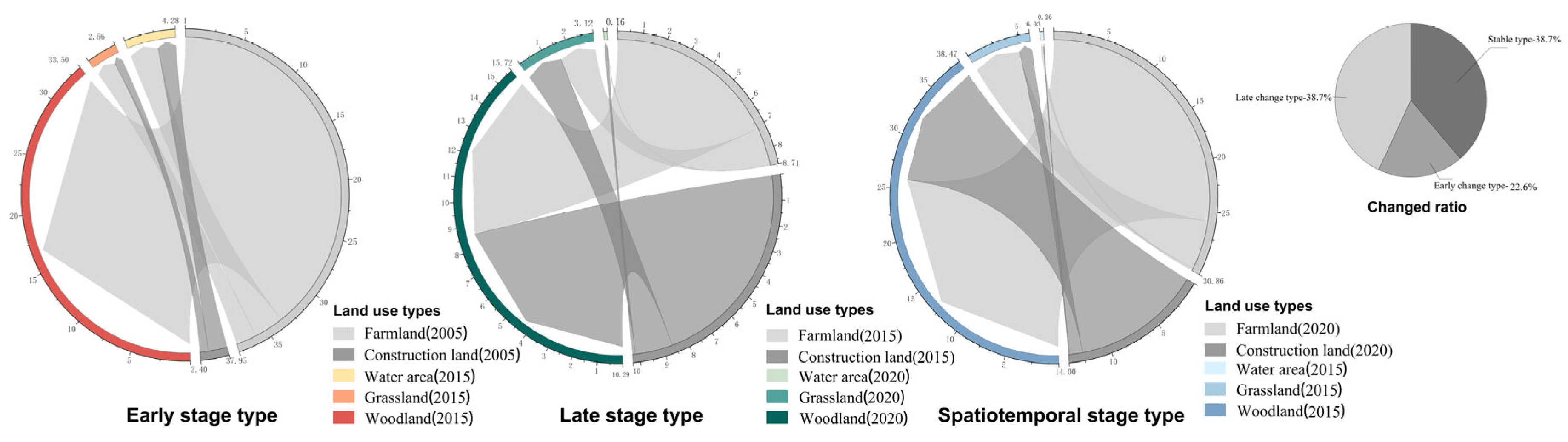
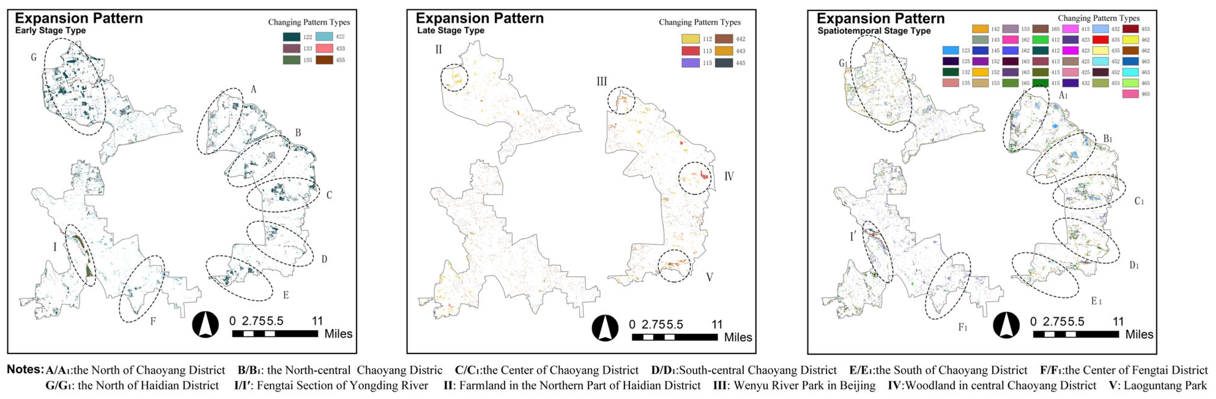
Expansion Patterns of Green Space

The expansion patterns of green spaces refers to the transition where non-green land-use types morph into green space land-use types, resulting in an augmented green space area. This encompasses the transformation of farmlands, construction lands, and unused lands into green space land-use types across different periods.

Mirroring the contraction pattern of green spaces, the expansion pattern classifies the top 15 transformation types into 3 pattern types: early transformation type, late transformation type, and spatiotemporal transformation type, as depicted in

Table 3. Land-use change of green space expansionin the boundary area between two green belts from 2005 to 2020.

Expansion Pattern	Time	Changing Time	Pattern-Change Illustration	Changed Area/km2	Changed Ratio/%
Early-stage type	2005–2015	1	a-b-b	40.36	38.72
Late-stage type	2015–2020	1	a-a-b	19.01	18.24
Spatiotemporal change type	2005–2020	2	a-b-c/a-b-a	44.87	43.04

. Among these three pattern types, the spatiotemporal transformation type represents the highest proportion (43.04%), implying that over 15 years, land areas that experienced varied land-use transitions before eventually evolving into green spaces exceeded the land areas that transformed into green spaces at any single point. This observation potentially provides evidence for the sustained greening efforts of Beijing’s million-acre afforestation over a 15 year span. Furthermore, the policy of returning farmland to forests implemented in Beijing throughout these 15 years had a significant impact on the urban green space pattern, particularly from 2005 to 2015. In the early transformation type, land areas converted from farmland to green spaces considerably outnumbered those from construction land, accounting for a hefty 83.03%. Moreover, all the converted forest lands originated from farmland types. This trend persisted from 2015 to 2020, with nearly half of the total conversion area stemming from the transformation of construction land into green spaces, given the scarcity of farmland in the interlacing zone (Figure 5).

In terms of the land-use types within green spaces, forest land predominates as the land-use type transitioning into green space combined with Figure 5. The area and proportion for each transformation pattern are as follows: in the early transformation pattern, the area is 35.51 km², accounting for 91.71%; in the late transformation pattern, the area is 15.73 km², accounting for 82.75%; in the spatiotemporal transformation pattern, the area is 38.48 km², accounting for 85.76%. These results suggest that afforestation is the primary approach to urban greening in the execution of urban ecological planning and construction. On the one hand, it contributes to the urban tree canopy environment and mitigates the urban heat island effect. On the other hand, for the rapidly contracting water bodies and grasslands, urban greening may not offer targeted solutions to their shrinkage issues. Thus, a singular approach may not suffice for ecological restoration of land use.

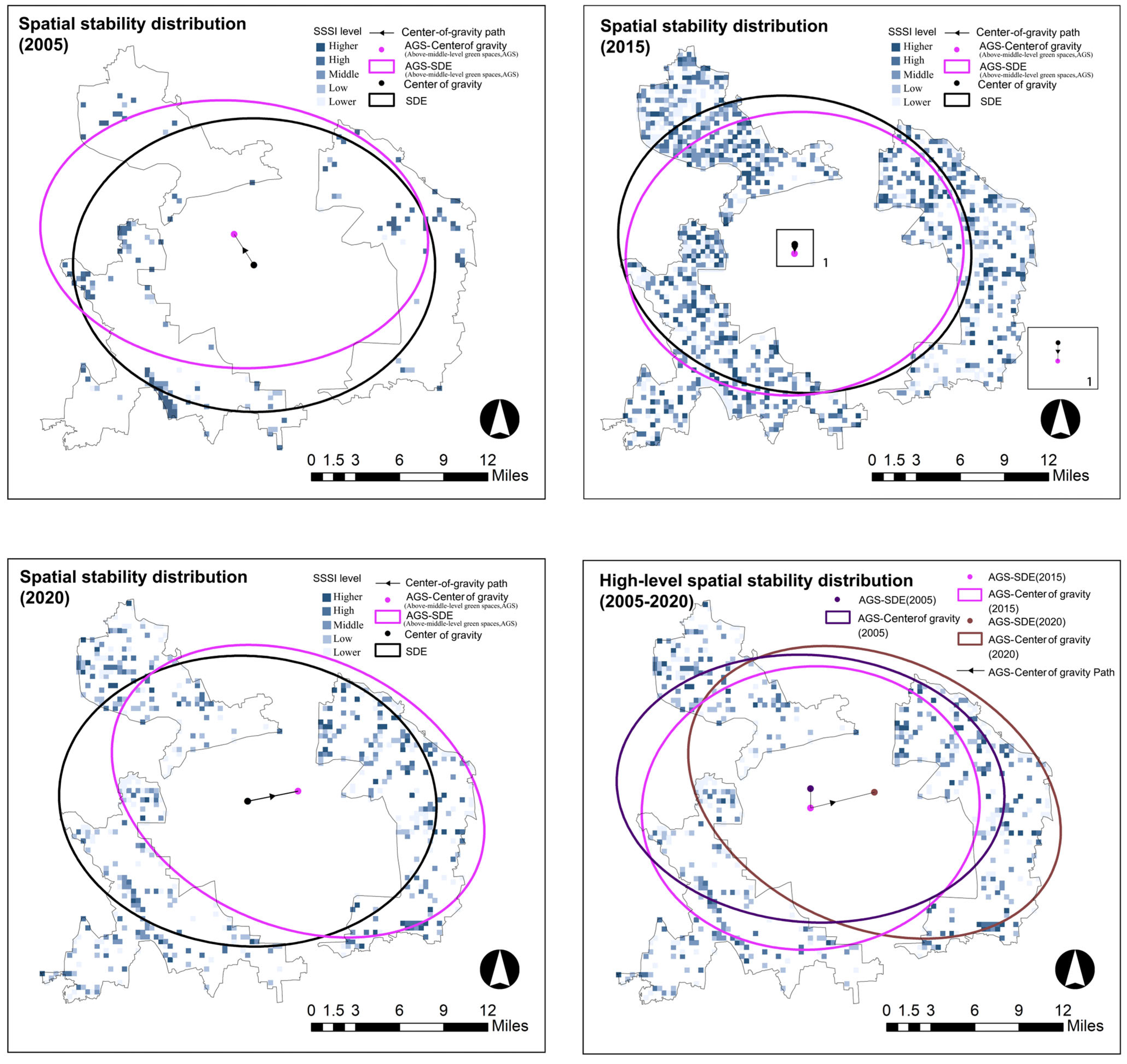
6.2.2. Analysis of Green Space Feature Distribution

Characteristics of Spatially Aggregated Effect

The phenomenon of land-use types’ agglomeration, wherein a non-uniform distribution is observed, forms the subject of this discussion. Utilizing the capabilities of the ArcGIS 10.2 software raster calculator, calculations were performed on the land-use map formula that pertains to the period between 2005 and 2020. Subsequent analysis of the agglomeration of green space was conducted via scrutiny of the green barrier-interlaced belt. The three-digit coding legend embodied in Figure 6 demarcates, from left to right, the land types for the years 2005, 2015, and 2020. Five land types are denoted by numerical codes as follows: farmland (1), woodland (2), grassland (3), construction land (4), water area (5), and bare land (6). Codes 2, 3, and 5 are categorized as green space land types, while 1 and 4 represent non-green space land types.

Agglomeration Characteristics of Green Space Contraction Mode. Depicted in Figure 6 are geospatial maps illustrating various patterns of land change. Within the stable pattern, the conversion of green spaces predominantly occurs in the western sector of the second green belt, the northern portion of Chaoyang District in the east, particularly the hybrid zone of farmland and residential areas proximate to the Second Airport Expressway, along with a modest conversion of green space on the southern bank of the Wenyu River in Yan’an District. High aggregation areas are characterized by regions I, II, and A, whereas regions B, C, and III denote medium aggregation areas, exhibiting a comparatively reduced aggregation range and conversion area. Under the early change type, a distinct wedge-shaped, high aggregation distribution pattern from the outskirts to the suburbs is observed in region IV. Regions D, E, and F are classified as medium aggregation areas. Conversely, the land area in other regions is limited and fragmented. Over the entire period, three high-aggregation areas are identified, namely, the Yongding River section of Fengtai, the Yongding River section of Shijingshan, and the Jingshan Park-Feicui Lake section in Chaoyang District.

Four transformation modes are present, with three high-aggregation areas observed in the entire period, as previously mentioned. The Yongding River Fengtai section and the shallow mountainous area near the western Fifth Ring Road in Shijingshan are linked to three transformation modes, represented by regions labeled as I, I′, I″, and II, II′, II″. Conversely, Lao Shan urban leisure park and the green space of the Jianguo Park-Feicui Lake section are connected to two transformation modes, represented by regions III, III′ and IV, IV′. This implies a potent tendency for the green space land types in these four regions to “shrink” synchronously with the progression of time and space, thus underlining the necessity for meticulous land management and control.

Agglomerative Characteristics of Green Space Expansion Modes. In contrast to the aggregation characteristics of the contraction mode, the expansion mode of the green barrier-interlacing space exhibits distinct distribution patterns in the early- and complete-change types. The three-digit coding legend in Figure 7 represents the land types in the years 2005, 2015, and 2020, moving from left to right. Numerical codes designate five land types: farmland (1), woodland (2), grassland (3), construction land (4), water area (5), and bare land (6). Green space land-type codes are represented by 2, 3, and 5, whereas non-green space land-type codes are signified by 1 and 4.

Referring to Figure 7, in the early change type (2005–2015), regions A through G demonstrate a distinct centripetal trend, whereas region I follows a horizontally connected trend. This pattern fundamentally establishes the “contraction–expansion” changes in the green barrier-interlacing space. In the late-change type (2015–2020), there is an absence of any potent aggregation trend forming a large area. Instead, only a few localized, small-scale aggregation distributions (II to V) are observed, and their specific locations do not deviate from the aggregation areas of the early change type. In the complete-change type (2005–2020), the distribution of the “expansion” of the green space essentially extends the base pattern of the early change type, with the “expansion” change occurring on its periphery.

A noteworthy point is the temporal and spatial evolution of the land types in the Fengtai section of the Yongding River, predominantly characterized by two aspects: First, under the “contraction” and “expansion” modes of green space, this area exhibits strong transformation and aggregation distribution on the type dimension. Second, irrespective of whether it is the early or complete period of change, this area exhibits persistent transformation in the time dimension.

Characteristics of Space Stability

The Spatial Structure Stability Index (SSSI) is derived from the Spatial Structure Conflict Index (SCCI), integrating the Spatial Complexity Index (CI), Spatial Vulnerability Index (FI), and Spatial Stability Index (SI). These components collectively assess the stability of spatial form, considering perspectives of morphological differentiation, land resilience, and stability. This section employs the Standard Deviational Ellipse (SDE) analysis method to examine the overall distribution trend of SSSI and high SSSI within the green space interlacing belt from 2005 to 2020, encompassing alterations in stability gravity center, distribution direction, and distribution shape.

Gravity Center of Distribution. As Figure 8 shown, in 2005, the distribution gravity center for high stability shifted northwestward relative to the overall stability center, indicating a denser distribution of high-stability green spaces in the northwest direction of the two green belts. This region primarily comprises continuous forests and grasslands, manifesting a high-quality ecological environment. By 2015, the high-stability center of gravity made a slight southward shift in comparison to the overall stability center of gravity. Although the total green space area experienced a significant increase, the enhancement of green space quality in the southern Yongding River basin positively impacted its center of gravity. In 2020, the high-stability center of gravity made a considerable eastward shift to the north of Chaoyang District. From 2005 to 2020, the high-stability center of gravity initially migrated slightly southward from the northwest, ultimately settling in the northeast. Broadly speaking, the stability of the northern green space is notably higher than that of the southern green space. Moreover, the change in its center of gravity is profoundly influenced by the temporal constraints of green space planning and construction. The northwest suburbs, benefited by their superior historical ecological environment, possess a robust ecological barrier and environmental foundation, causing an obvious bias in the green space’s center of gravity during the early phase of urban construction. However, the center of gravity has since moved southward, influenced by urban planning policies, such as the construction of Beijing’s Yizhuang New City and the development of Beijing’s sub-center.

Distribution shape. The distribution shape is primarily scrutinized through alterations in the major and minor axes of the standard deviation ellipse and their ratio (Figure 9). A larger axis ratio denotes prominent directional characteristics and vice versa. As depicted in Figure 8, from 2005 to 2020, the SSSI values in the region are generally evenly distributed. The ratio of the major and minor axes of the standard ellipse is generally small, with flatness ranging between 1 and 1.5. The major–minor axis ratio of high SSSI and overall SSSI in 2005 and 2020 exceeded that in 2015, suggesting that the spatial stability of the region’s form in 2005 and 2020 was more directionally oriented and exhibited a stronger northwest direction.

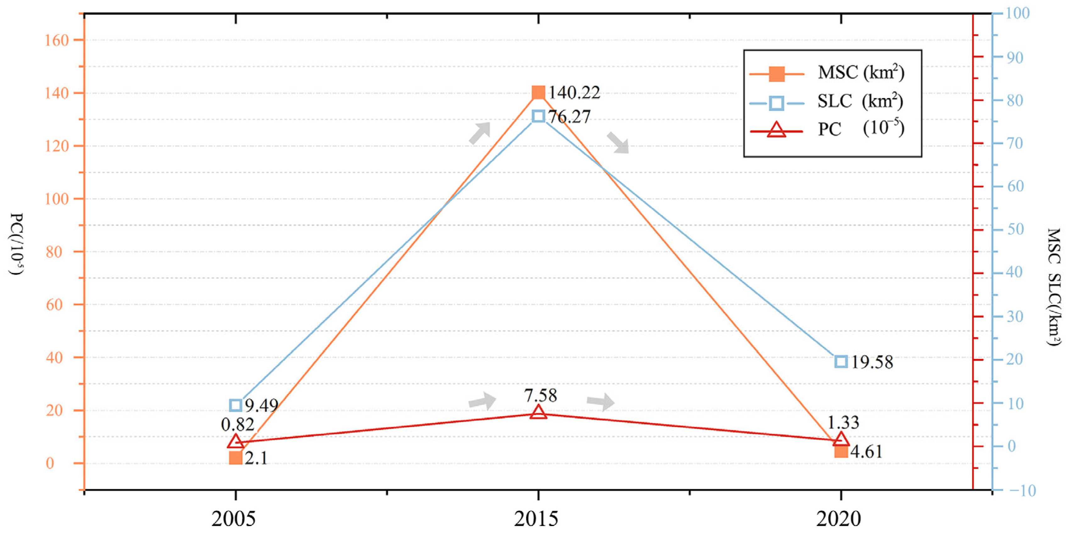
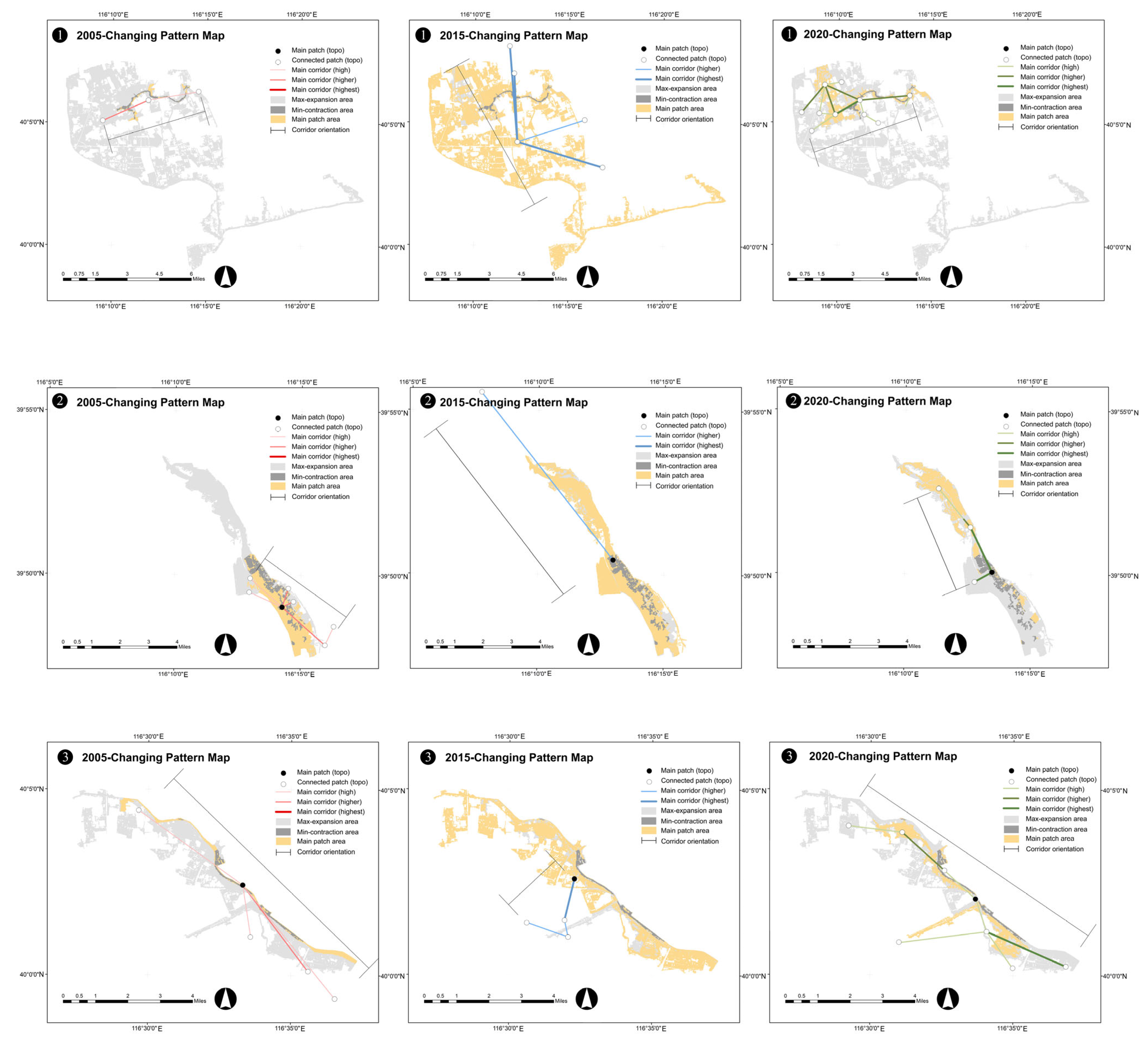
6.2.3. Analysis of Green Space Connectivity Level

Global connectivity. The connectivity indicators (PC, SLC, MSC) of green interlaced belts and green space land use from 2005 to 2020 are depicted in Figure 10. Between 2005 and 2020, the global connectivity level (PC) was noted to have remained stable, with 2015 witnessing a marginal increase compared to the other two years. In 2015, the SLC value exhibited a significant rise compared to 2005 and 2020, indicative of the enhanced dominance and aggregation of the largest patches of green space in 2020. An elevated MSC value was observed in 2015 compared to other years, signalling superior average connectivity for that year (Figure 10).

Local connectivity. The year 2020 was characterized by the highest level of connectivity at nodes, compared to 2005 and 2015, with the fewest in 2005. As for connectivity corridors, their densest distribution and strongest connectivity were recorded in 2015, followed by 2020, with 2005 observing the least.

In 2005, a pattern of “three dominant positions, overall scattered distribution” was evident in the distribution of connectivity nodes and corridors. These dominant positions were predominantly distributed at the high-connectivity nodes and high corridor connectivity characteristics of the Wenyu River Chaoyang section, the North West Mountain Plain in Haidian district, and the Yongding River Fengtai section. The distribution of connectivity nodes and corridors in 2015 adopted a “one dominant position, three cores, and overall density” pattern. This “one dominant position” is a reflection of the complex and radially distributed network characteristics of multiple centers in the northwest suburban plain area of Haidian district. The area encircling the Cuihu National Urban Wetland Park as the core node boasted the strongest connectivity, displaying strong connectivity to both the north and south and forming a gradient difference. The “three cores” relate to the Yongding River Fengtai section, the Wenyu River Chaoyang North section, and the Jiufu Park group. Notably, the corridor connectivity and length of the Yongding River Fengtai section experienced considerable enhancement, extending from the north to Shijingshan Park in Shijingshan district and to the south to World Park in Fengtai district. In 2020, the distribution of connectivity nodes and corridors adopted a “multi-center, short corridors, and even distribution” pattern.

While varying characteristics of local connectivity in the study area have been observed from 2005 to 2020, it is noteworthy that high connectivity has been consistently maintained in the green spaces of the north of Haidian district (Label 1), the northwest of Fengtai district (Label 2), the middle of Chaoyang district (Label 3), and the middle of Haidian district (Label 4) during the pronounced “contraction–expansion” pattern of change. Particularly, the green spaces in the north of Haidian district (Label 1), the northwest of Fengtai district (Label 2), and the middle of Chaoyang district (Label 3) have managed to preserve high connectivity amidst the dramatic “contraction–expansion” pattern, As illustrated in Figure 11.

As illustrated in Figure 12, a linear pattern is exhibited by areas 2 and 3, which continues to be upheld in the “contraction–expansion” change pattern, while the linear region in area 1 sustains a stable pattern post-2015, exerting significant influence on the corridor orientation characteristics of the area. In this linear pattern, the distribution of its high-connectivity corridors is distinctly characterized by a unidirectional trend. Among them, the corridor distribution tendencies of the three regions in 2005 and 2020 align with the overall linear pattern. Remarkable reversals (regions 1, 3) and modification (region 2) in the direction of their corridor distribution were discernible in 2015.

7. Discussion

Drawing upon the principles of landscape ecology, this study quantifies the ecological value of a given area via the land-use alterations within green space interlaced belts. The spotlight is on the proactive transformation patterns of the green space as the primary subject, rather than the passive modifications incited by urban expansion. The emergence of the “contraction–expansion” alteration mechanism in green spaces is governed by the interaction of two factors—the propagation of construction land under urban economic construction and the drive from urban ecological policies for green construction. This dynamic interplay not only affects the transformation of green space and non-green space land-use types but also alters the internal structure of the green space. This is the fundamental mechanism whereby present circumstances and planning concurrently stimulate the urban land pattern.

A prevalent global solution involves constructing extensive green belts within urban built-up areas to deter the haphazard spread of urban land. However, discussions regarding the ecological value and transitional nature of green spaces within these green belts, neglecting their unique “urban” attribute, are often scarce. On the contrary, intense land conflicts frequently hinder the execution of such construction. Hence, the value of green spaces as urban land that can be “cut” lacks equitable treatment, underscoring the need for a scientific identification methodology and value expression that can effectively validate the worth of green spaces for planning and construction of unique transitional green spaces.

The spatiotemporal evolution pattern of the “contraction–expansion” mechanism at the boundary between two green belts aligns with the overall developmental trajectory of Beijing’s urban growth. Post-2015, Beijing transitioned into a phase of urban economic development and ecological construction, which essentially accounts for the emergence of the “contraction–expansion” mechanism at the boundaries between two green belts. Moreover, empirical evidence of the considerable “expansion” of forest land highlights that the implementation of a single green space plan negatively impacts other green spaces, such as significantly reducing water space, necessitating adequate attention. The non-circular pattern and the deviation of the center of gravity exhibited by the interspersion zone space reveal an inequitable distribution of green spaces across different regions. This disparity may reflect the strategic layout differences among varying administrative regions, implying that advocating for a green space compensation mechanism across diverse regions could be more significant than establishing an absolute circular pattern based on green space fairness. This study emphasizes the identification of ecological source areas as crucial connectivity nodes in the formation of a green network, expanding beyond the existing binary judgments of “quality” and “quantity” and concentrating on the integrated regional ecological network planning mode encompassing “space” and “relationship”.

8. Conclusions

Over a span of 15 years, the area witnessed a 10% increase in construction land, consequently triggering a significant metamorphosis in urban green space from “expansion” to “contraction”. This transformation was particularly salient within the land-use structure during the same epoch. For instance, the considerable “expansion” of green space from 2005 to 2015 bears testament to the successful implementation of Beijing’s urban planning policies, which were designed to “curb” urban sprawl. Post-2015, however, the trend of urban construction land proliferation became more pronounced, and the ensuing “contraction” of urban green space became readily apparent. Concurrently, a peculiar phenomenon of temporal and spatial repeated transformation of certain green space areas was observed. Despite these land patches being relatively small, their perpetual alteration and fragmentation within the geographical space call for scrutiny from land management authorities. Broadly speaking, between 2005 and 2020, the green space within the green belt interlaced zone underwent an “expansion-contraction” trajectory, exhibiting a marked shift in land pattern around 2015. As far as the morphological characteristics of green space are concerned, despite different types of green space land exhibiting diverse transformation outcomes under varying transformation modalities, they manifested similar aggregation effects within the geographical space. This study counters the prior singular notion of either stability or instability explored at the medium scale, implying that land can concurrently exhibit characteristics of stability and extreme instability at this scale. In the evolution of expanding green space, there was also a conspicuous aggregation effect observable in the spatial morphology, such as the emergence of five evenly distributed wedge-shaped and longitudinal green space forms in Chaoyang District, which are the outcome of superior-level land planning. The stability, the high stability gravity center, and the standard deviation elliptical shape and direction were shaped by the urban historical ecological texture in its early stage, and the greenification initiatives and ecological strategies of different urban sections significantly remolded the spatial stability. Land connectivity also displayed a crucial shift around 2015. Furthermore, this study highlighted three directionally significant distribution nodes, which have been instrumental in fostering connectivity amidst the vast spatiotemporal evolution of the land, bridging disparate green space units, and shaping the corridor distribution dynamics.

References

1. Islam, M.N.; Rahman, K.-S.; Bahar, M.M.; Habib, M.A.; Ando, K.; Hattori, N. Pollution attenuation by roadside greenbelt in and around urban areas. Urban For. Urban Green. 2012, 11, 460–464. [Google Scholar] [CrossRef]
2. Kowarik, I. The “Green Belt Berlin”: Establishing a greenway where the Berlin Wall once stood by integrating ecological, social and cultural approaches. Landsc. Urban Plan. 2019, 184, 12–22. [Google Scholar] [CrossRef]
3. Pathak, V.; Tripathi, B.D.; Mishra, V.K. Evaluation of Anticipated Performance Index of some tree species for green belt development to mitigate traffic generated noise. Urban For. Urban Green. 2011, 10, 61–66. [Google Scholar] [CrossRef]
4. Yang, J.; Jinxing, Z. The failure and success of greenbelt program in Beijing. Urban For. Urban Green. 2007, 6, 287–296. [Google Scholar] [CrossRef]
5. Immergluck, D.; Balan, T. Sustainable for whom? Green urban development, environmental gentrification, and the Atlanta Beltline. Urban Geogr. 2018, 39, 546–562. [Google Scholar] [CrossRef]
6. Ramesh, R.M.; Nijagunappa, R. Development of urban green belts—A super future for ecological balance, Gulbarga city, Karnataka. Int. Lett. Nat. Sci. 2014, 27, 47–53. [Google Scholar] [CrossRef]
7. Xie, X.; Kang, H.; Behnisch, M.; Baildon, M.; Krüger, T. To What Extent Can the Green Belts Prevent Urban Sprawl?—A Comparative Study of Frankfurt am Main, London and Seoul. Sustainability 2020, 12, 679. [Google Scholar] [CrossRef]
8. Dou, Y.; Kuang, W. A comparative analysis of urban impervious surface and green space and their dynamics among 318 different size cities in China in the past 25 years. Sci. Total Environ. 2020, 706, 135828. [Google Scholar] [CrossRef]
9. Han, H.; Huang, C.; Ahn, K.-H.; Shu, X.; Lin, L.; Qiu, D. The Effects of Greenbelt Policies on Land Development: Evidence from the Deregulation of the Greenbelt in the Seoul Metropolitan Area. Sustainability 2017, 9, 1259. [Google Scholar] [CrossRef]
10. Kardani-Yazd, N.; Kardani-Yazd, N.; Mansouri Daneshvar, M.R. Strategic spatial analysis of urban greenbelt plans in Mashhad city, Iran. Environ. Syst. Res. 2019, 8, 30. [Google Scholar] [CrossRef]
11. Kuang, W.; Chi, W.; Lu, D.; Dou, Y. A comparative analysis of megacity expansions in China and the U.S.: Patterns, rates and driving forces. Landsc. Urban Plan. 2014, 132, 121–135. [Google Scholar] [CrossRef]
12. Sun, L.; Chen, J.; Li, Q.; Huang, D. Dramatic uneven urbanization of large cities throughout the world in recent decades. Nat. Commun. 2020, 11, 5366. [Google Scholar] [CrossRef] [PubMed]
13. Elmqvist, T.; Andersson, E.; McPhearson, T.; Bai, X.; Bettencourt, L.; Brondizio, E.; Colding, J.; Daily, G.; Folke, C.; Grimm, N.; et al. Urbanization in and for the Anthropocene. NPJ Urban Sustain. 2021, 1, 6. [Google Scholar] [CrossRef]
14. Xu, G.; Jiao, L.; Liu, J.; Shi, Z.; Zeng, C.; Liu, Y. Understanding urban expansion combining macro patterns and micro dynamics in three Southeast Asian megacities. Sci. Total Environ. 2019, 660, 375–383. [Google Scholar] [CrossRef]
15. Zhao, S.; Zhou, D.; Zhu, C.; Qu, W.; Zhao, J.; Sun, Y.; Huang, D.; Wu, W.; Liu, S. Rates and patterns of urban expansion in China’s 32 major cities over the past three decades. Landsc. Ecol. 2015, 30, 1541–1559. [Google Scholar] [CrossRef]
16. Li, F.; Wang, R.; Paulussen, J.; Liu, X. Comprehensive concept planning of urban greening based on ecological principles: A case study in Beijing, China. Landsc. Urban Plan. 2005, 72, 325–336. [Google Scholar] [CrossRef]
17. Ma, M.; Jin, Y. What if Beijing had enforced the 1st or 2nd greenbelt?—Analyses from an economic perspective. Landsc. Urban Plan. 2019, 182, 79–91. [Google Scholar] [CrossRef]
18. Sun, L.; Fertner, C.; Jørgensen, G. Beijing’s First Green Belt—A 50-Year Long Chinese Planning Story. Land 2021, 10, 969. [Google Scholar] [CrossRef]
19. Chen, J.; Han, S.S.; Chen, S. Understanding the structure and complexity of regional greenway governance in China. Int. Dev. Plan. Rev. 2022, 44, 241–264. [Google Scholar] [CrossRef]
20. Cheng, J.; Turkstra, J.; Peng, M.; Du, N.; Ho, P. Urban land administration and planning in China: Opportunities and constraints of spatial data models. Land Use Policy 2006, 23, 604–616. [Google Scholar] [CrossRef]
21. Ma, L.J.C. Urban administrative restructuring, changing scale relations and local economic development in China. Political Geogr. 2005, 24, 477–497. [Google Scholar] [CrossRef]
22. Chu, M.; Lu, J.; Sun, D. Influence of Urban Agglomeration Expansion on Fragmentation of Green Space: A Case Study of Beijing-Tianjin-Hebei Urban Agglomeration. Land 2022, 11, 275. [Google Scholar] [CrossRef]
23. Jiao, L.; Xu, G.; Xiao, F.; Liu, Y.; Zhang, B. Analyzing the Impacts of Urban Expansion on Green Fragmentation Using Constraint Gradient Analysis. Prof. Geogr. 2017, 69, 553–566. [Google Scholar] [CrossRef]
24. Li, K.; Li, C.; Liu, M.; Hu, Y.; Wang, H.; Wu, W. Multiscale analysis of the effects of urban green infrastructure landscape patterns on PM2.5 concentrations in an area of rapid urbanization. J. Clean. Prod. 2021, 325, 129324. [Google Scholar] [CrossRef]
25. Liu, K.; Li, X.; Wang, S.; Gao, X. Assessing the effects of urban green landscape on urban thermal environment dynamic in a semiarid city by integrated use of airborne data, satellite imagery and land surface model. Int. J. Appl. Earth Obs. Geoinf. 2022, 107, 102674. [Google Scholar] [CrossRef]
26. Tian, Y.; Jim, C.Y.; Wang, H. Assessing the landscape and ecological quality of urban green spaces in a compact city. Landsc. Urban Plan. 2014, 121, 97–108. [Google Scholar] [CrossRef]
27. Yang, J.; Huang, C.; Zhang, Z.; Wang, L. The temporal trend of urban green coverage in major Chinese cities between 1990 and 2010. Urban For. Urban Green. 2014, 13, 19–27. [Google Scholar] [CrossRef]
28. Zhao, J.; Chen, S.; Jiang, B.; Ren, Y.; Wang, H.; Vause, J.; Yu, H. Temporal trend of green space coverage in China and its relationship with urbanization over the last two decades. Sci. Total Environ. 2013, 442, 455–465. [Google Scholar] [CrossRef]
29. Qiong, W.; Bin, W.; Shenjun, Y.; Jianping, W.; Ying, Z.; Jing, Z. Evolution and change of an urban greenspace: A case study on the outer ring of Shanghai. J. East China Norm. Univ. Nat. Sci. 2021, 2, 100–109. [Google Scholar]
30. Kowe, P.; Mutanga, O.; Dube, T. Advancements in the remote sensing of landscape pattern of urban green spaces and vegetation fragmentation. Int. J. Remote Sens. 2021, 42, 3797–3832. [Google Scholar] [CrossRef]
31. Cohen, J. A Coefficient of Agreement for Nominal Scales. Educ. Psychol. Meas. 1960, 20, 37–46. [Google Scholar] [CrossRef]
32. Shupeng, C. Geographical data handling and GIS in China. Int. J. Geogr. Inf. Syst. 1987, 1, 219–228. [Google Scholar] [CrossRef]
33. Bao, W.; Yang, Y.; Zou, L. How to reconcile land use conflicts in mega urban agglomeration? A scenario-based study in the Beijing-Tianjin-Hebei region, China. J. Environ. Manag. 2021, 296, 113168. [Google Scholar] [CrossRef] [PubMed]
34. Li, X.; Lu, L.; Cheng, G.; Xiao, H. Quantifying landscape structure of the Heihe River Basin, north-west China using FRAGSTATS. J. Arid Environ. 2001, 48, 521–535. [Google Scholar] [CrossRef]
35. Foltête, J.-C.; Clauzel, C.; Vuidel, G. A software tool dedicated to the modelling of landscape networks. Environ. Model. Softw. 2012, 38, 316–327. [Google Scholar] [CrossRef]
36. Shi, N.; Guo, N.; Liu, G.; Wang, Q.; Han, Y.; Xiao, N. Spatial distribution pattern and influencing factors of amphibians and reptiles in Beijing. ACTA Eologinca Sin. 2022, 42, 3806–3821. [Google Scholar]
37. Li, H.; Chen, H.; Wu, M.; Zhou, K.; Zhang, X.; Liu, Z. A Dynamic Evaluation Method of Urban Ecological Networks Combining Graphab and the FLUS Model. Land 2022, 11, 2297. [Google Scholar] [CrossRef]
Figure 1. Study area.
Land 12 01621 g001
Figure 2. Framework of the multi-index system.
Land 12 01621 g002
Figure 3. Land use classification map (2005–2020).
Land 12 01621 g003
Figure 4. Sankey diagram of green space contraction pattern in the boundary area.
Land 12 01621 g004
Figure 5. Sankey diagram of green space expansion pattern in the boundary area.
Land 12 01621 g005
Figure 6. Spatial agglomerations of contraction pattern in the green space (2005–2020).
Land 12 01621 g006
Figure 7. Spatial agglomerations of expansion pattern in the green space (2005–2020).
Land 12 01621 g007
Figure 8. Gravity center of distribution.
Land 12 01621 g008
Figure 9. Distribution shape of green space in the boundary area, 2005–2020.
Land 12 01621 g009
Figure 10. Changes in green space connectivity at the global level, 2005–2020.
Land 12 01621 g010
Figure 11. Changes in green space connectivity at the local level, 2005–2020.
Land 12 01621 g011
Figure 12. Characterization of “contraction–expansion” changes in the area and corridor changes in three important regions.
Land 12 01621 g012