Integrated Modeling of Land Degradation Dynamics and Insights on the Possible Future Management Alternatives in the Gidabo River Basin, Ethiopian Rift Valley

Abstract

Land degradation is a pivotal environmental concern, bearing substantial impacts in the Gidabo river basin (GRB) in Ethiopia, prompting a critical need for effective mitigation strategies. In this study, we aimed to assess the dynamics of land degradation pathways in the context of change in climate and land use. The identification of potential erosion hotspots and the appraisal of management strategies was also carried out. The Soil and Water Assessment Tool (SWAT) and the Good Practice Guidance (GPG) framework was employed. The results revealed a compelling synergy between land use dynamics and climate changes, asserting joint and individual prevalence in influencing surface runoff and sediment yield. The past simulation revealed 4–5.9% and 24–43% increments in mean annual runoff and sediment yield, respectively. While the near (2021–2040) and mid (2041–2060) future scenarios displayed varying trends under RCP4.5 and RCP8.5. Furthermore, sub-basins prone to soil erosion risk were identified, thereby enabling targeted conservation efforts. The assessment of trends in land degradation neutrality (LDN) unveiled the expansion of land degradation trajectories (by 26%) from 1985–2003 to 2003–2021. This might be attributed to the dynamic interplay between climate and land use land cover (LULC) change, with croplands and bare land emerging as high-risk degraded areas. Addressing these concerns, soil/stone bund, terracing, contour farming, and reforestation practice can significantly reduce the annual sediment yield in the future. The integration of soil erosion indicators with LDN sub-indicators can provide a more comprehensive approach that can lead to more effective land management and restoration strategies to achieve the LDN goal. The findings of this study could contribute crucial insights and substantial implications for policymakers, land managers, and conservationists. Moreover, future efforts should be directed to expand investigations into diverse land degradation pathways and mitigation measures.

1. Introduction

Land has the potential to provide a full suite of goods and services at local, landscape and global scale [1,2]. Nevertheless, land is coming under growing pressure from ever-increased competing uses [3] and subjected to increasing degradation trends [2]. Land degradation has diverse and wide-reaching impacts on the provision of vital ecosystem services, causing economic and social consequences more severely than ever before [4,5,6,7]. These impacts, however, are worse in developing countries, where the majority of the population directly depends on land resources for its livelihood [8,9]. Most of East Africa, including Ethiopia, has experienced severe land degradation problems that pose a challenge to people’s livelihoods [8,10,11]. Different approaches have been used to assess land degradation including expert opinions, field measurement, biophysical modeling and remote sensing, or a combination thereof [11,12,13].

The expert opinion approach highly relied on the people consulted and is considered subjective, inconsistent and replicable with difficulty [13,14]. Field measurement involves local sampling techniques and surveys to provide detailed objective information, for example, at a plot level [13]. However, this approach is often criticized for being time-consuming, labour intensive, costly and applicable to small areas [13]. The biophysical modeling approach integrate biophysical variables to assess land degradation. Though it is globally consistent and quantitative, its accuracy might be influenced by inherent error [13,14]. The remote sensing approach is vital in measuring land degradation, especially over a larger scale [11,15]. Remote sensing provides a plausible, consistent and useful alternative for multi-temporal and operational scale monitoring of land degradation. This approach is considered a cost-effective, reputable and time-efficient [14].

Most recently, the United Nations Convention to Combat Desertification (UNCCD) introduced the concept of “Land Degradation Neutrality” (LDN) to combat and recover the current trends in land degradation [16]. LDN that refers to a condition of “zero net land degradation” became one of the significant targets of the Sustainable Development Goal (SDG 15.3). An extensive description of LDN is provided in [17,18]. The LDN assessment is based on three significant biophysical sub-indicators: (i) land productivity (LP), (ii) land cover (LC) and (iii) soil organic carbon (SOC) [17]. The three indicators follow the principle of “The One-Out, All-Out (1OAO)” [18,19]. This principle enables the identification of land degradation more accurately with three dimensions of land status including aboveground, below-ground, and surface change [19]. Trends.Earth, a QGIS plugin, is working in combination with the Google Earth Engine to facilitate data preparation and processing for generating both the sub-indicators and the final SDG indicator 15.3.1 [20].

Soil erosion is a widely distributed land degradation pathway and an important complement to the three global LDN indicators that interacts with other environmental issues [21,22]. In recent decades, with the well-established use of geospatial technologies, models are becoming increasingly important in the identification of erosion prone areas at different time and spatial scales [23,24,25]. Process-based hydrological models are very accurate owing to their capabilities to simulate and describe the spatial distribution of land degradation [4]. These models can depict the spatial characters of meteorological conditions, topography, land cover and soil properties [24]. The soil and water assessment tool (SWAT) model, the most widely used model [23], considers these factors to identify areas susceptible to soil erosion [26]. SWAT model provides spatial and temporal distribution and magnitude of soil erosion and sediment load [4]. Moreover, the SWAT model allows to quantify the impact of land management practices and is capable of assessing the best management alternatives in large and complex watersheds [25].

The present study demonstrated an integrated approach to assess the trends of land degradation in the Gidabo river basin (GRB), located in the Ethiopian rift valley. The basin has been subjected to substantial landscape alteration, climatic variability and drastic ecological change [27,28,29,30,31,32]. These changes, triggered by dynamic population growth, exacerbate soil erosion, excessive sedimentation and eutrophication of waterbodies, hydrological imbalance and land–water–energy–food nexus resource degradation in the basin [33,34,35,36,37,38]. The explicit quantification of spatial and temporal trends of land degradation and its trajectory help to achieve LDN [15]. Moreover, decisions addressing land degradation problems are not only based on an assessment of the current land degradation but also on the expected future state of the land [4].

Climate and land use change are intertwined with soil erosion and land degradation. Understanding these interactions is crucial for developing effective strategies to achieve LDN goals. It is notable that land degradation can take many forms and that some methods are not appropriate for measuring all forms of land degradation pathways [11]. However, previous studies lack spatial and temporal information on the extent and magnitude of land degradation in the GRB. Therefore, this study aimed at the integration of SWAT model and Trends.Earth platform to assess land degradation pathways in the GRB. The specific objectives were to (1) extensively evaluate the individual and joint impacts of climate and land use land cover (LULC) change on runoff and soil erosion during the temporal span of 1990 to 2060, (2) conduct an in-depth assessment of trends in land degradation neutrality, (3) identify erosion hotspots necessitating intensified attention, and (4) evaluate potential management alternatives aimed at curtailing sediment production.

2. Materials and Methods

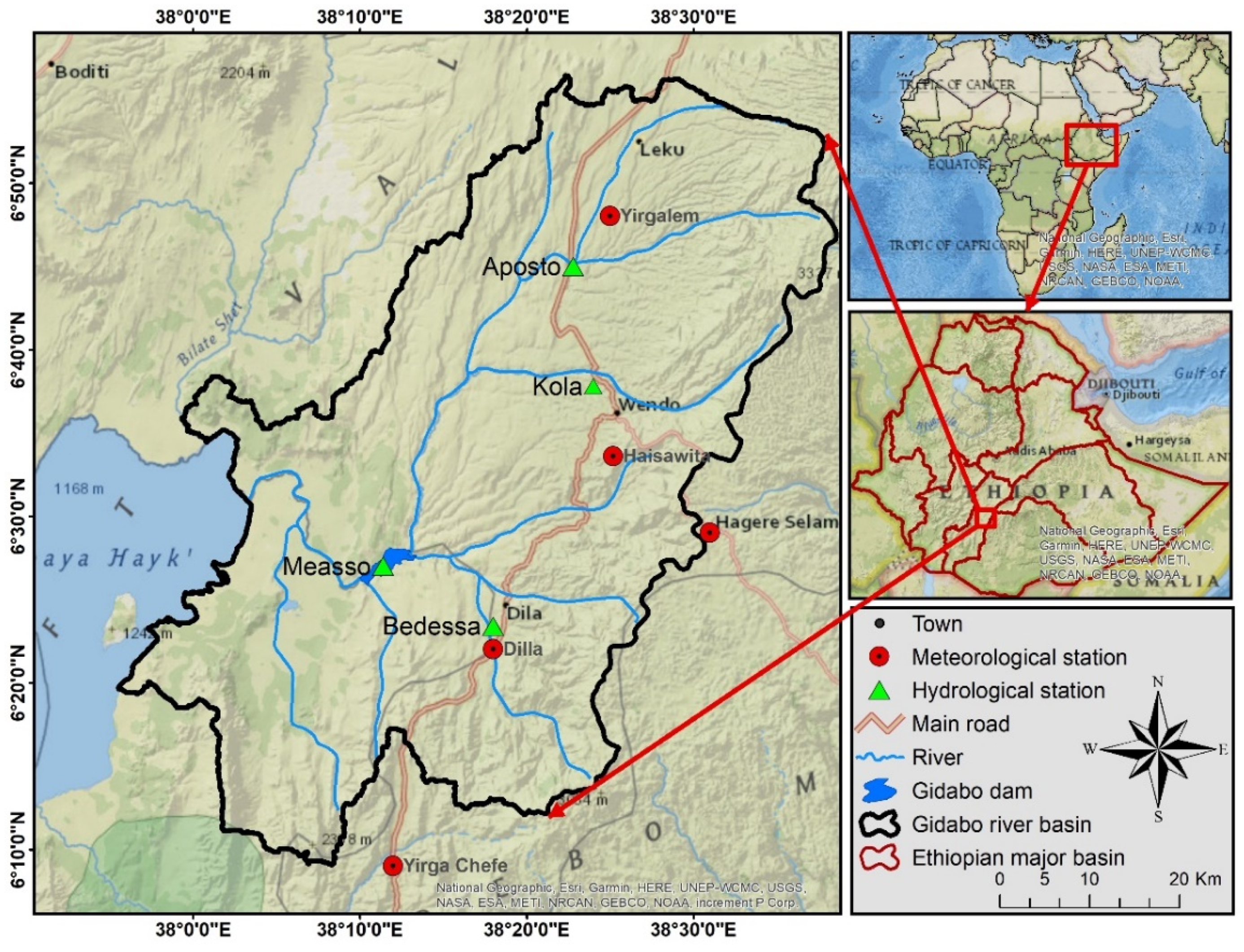
2.1. Description of the Study Area

The GRB is located in the Ethiopian main rift valley between 6°8′ N to 6°57′ N latitude and 37°0′ E to 38°40′ E longitude with approximately 3549 km² (Figure 1). GRB is characterized by its diverse biophysical composition with dendritic drainage patterns [27], flowing east–west into Lake Abaya. The area receives bimodal rainfall distribution (March–May and June–October) with mean annual rainfall of 1315 mm [39]. The average monthly temperature varies between 11 °C and 25 °C. Among the land uses, agriculture and agroforestry are the dominant contributors to the livelihood of the local community, resulting in increased trends with the expense of natural vegetation [30]. The population density increased towards the eastern highland and their livelihoods primarily depend on mixed crop-livestock farming system [35].

2.2. Data Source and Processing

2.2.1. Climate Data

The observed data of daily rainfall, temperature, solar radiation, relative humidity and wind speed were collected from 5 stations (Figure 1). The data were acquired from the Ethiopian Meteorology Institute (EMI) for the period of 1990–2021 and Dilla station was used to establish the weather generator database. Filling of missed meteorological data and temporal homogeneity test was performed using XLSTAT 2022.4 statistical software as used by previous studies [39,40,41]. Moreover, double mass curve (DMC) analysis was executed to assess the consistency of rainfall [42]. Projected climate data for near (2021–2040) and mid (2041–2060) future were acquired from Regional Climate Model (RCM) of Coordinated Regional Climate Downscaling Experiment (CORDEX) (https://esgf-data.dkrz.de/search/esgf-dkrz/ (accessed on 11 April 2022)). Two representative concentration pathways (RCP), i.e., moderate emission (RCP4.5) and highest emission (RCP8.5) were considered as future scenarios [43]. According to our performance study [39], RACMO22T (ECEARTH), CCLM4–8 (MPI), CRCM5 (MPI), CCLM4–8 (CNRM) and REMO2009 (EC-EARTH) were chosen. Thus, the ensemble of these RCMs was used and bias corrected using distribution mapping (DM) method. DM method provided better result in the study basin [31]. Moreover, Mann–Kendall (MK) test and Sen’s slope estimator were used to test the trends in climate variables. A detailed description of these trend test methods can also be found in Girma et al. [39].

2.2.2. Spatial Data

The long-term LULC dynamics for the baseline years (1985, 2003 and 2021) and projected years (2035 and 2050) were adopted from our recent study [30]. For erosion modeling, soil data were extracted from the latest FAO Harmonized World Soil Database version 2.0 (https://gaez.fao.org/pages/hwsd (accessed on 2 June 2023)) [44]. Additionally, the SoilGrids raster layer at 250 m spatial resolution developed by the International Soil Reference Information Center (ISRIC) was used for SOC estimation (https://soilgrids.org/ (accessed on 15 July 2023)). Topographic data were extracted from the Alaskan Satellite Facility digital elevation model (DEM) (12.5 m resolution) available at https://search.asf.alaska.edu/#/ (accessed on 20 June 2023).

2.2.3. Hydrology Data

For SWAT model calibration and validation, 18 years (1997–2014) daily streamflow data at Aposto and Bedessa gaging stations (Figure 1) were used. The two stations were considered since they have the longest period of flow data. The data were acquired from the Ministry of Water and Energy (MoWE) of Ethiopia. Due to the lack of continuous-time step sediment records, sediment yield data were generated using sediment rating curve (SRC). The SRC is extensively used to overcome the scarcity of temporal sediment data [45,46,47,48,49]. Hence, the suspended sediment load for Aposto and Bedessa gauging stations was generated using the sediment discharge rating curve developed by Adi et al. [48] with an R² value of 0.96 and 0.91, respectively.

2.3. Assessment of Land Degradation Indicators

2.3.1. Soil Erosion Modeling Using SWAT

To evaluate the effects of climate and LULC change, we applied 20 different simulations (individual and combined scenarios), as shown in

Table 1. SWAT model simulation setup.

Simulation	LULC	Climate	RCP
Past period
S1 *	1985	1990–2005	–
S2	2003	1990–2005	–
S3	2021	1990–2005	–
S4	1985	2006–2020	–
S5	2003	2006–2020	–
S6 **	2021	2006–2020	–
Future LULC change scenario
S7	2035	2006–2020	–
S8	2050	2006–2020	–
Future climate change scenario
S9	2021	2021–2040	RCP4.5
S10	2021	2041–2060	RCP4.5
S11	2021	2021–2040	RCP8.5
S12	2021	2041–2060	RCP8.5
Future combined (LULC and climate change) scenario
S13	2035	2021–2040	RCP4.5
S14	2035	2041–2060	RCP4.5
S15	2035	2021–2040	RCP8.5
S16	2035	2041–2060	RCP8.5
S17	2050	2021–2040	RCP4.5
S18	2050	2041–2060	RCP4.5
S19	2050	2021–2040	RCP8.5
S20	2050	2041–2060	RCP8.5

*, ** represents baseline for past period and future scenario, respectively.

. Prior to simulation, the study area was divided into sub-basins using the DEM as input in SWAT2012 (interface of ArcGIS10.8). Furthermore, each sub-basin was further subdivided into several number of hydrologic response units (HRUs) ¹ with a unique combination of 5% land cover, 10% soil type and 10% slope thresholds. Then, all the required climatic variables were fed to the model and a three-year warming-up period was given during simulation. Details of SWAT model procedure is given in SWAT theoretical documentation [50]. Surface runoff was estimated using the soil conservation service curve number (SCS-CN) method (Equation (1)) [50].

$${\mathrm{Q}}_{\mathrm{s}\mathrm{u}\mathrm{r}\mathrm{f}}=\frac{{\left({\mathrm{R}}_{\mathrm{d}\mathrm{a}\mathrm{y}}-0.2\mathrm{S}\right)}^2}{\left({\mathrm{R}}_{\mathrm{d}\mathrm{a}\mathrm{y}}+0.8\mathrm{S}\right)},$$

(1)

where Q_surf is the accumulated runoff (mm), R_day is the daily rainfall depth (mm water), and S is the retention parameter (mm water) mathematical expressed using the curve number (CN) (Equation (2)). The CN is governed mainly by LULC, soil permeability and a hydraulic group of soils [50].

$$\mathrm{S}=25.4\left(\frac{1000}{\mathrm{C}\mathrm{N}}-10\right),$$

(2)

Soil erosion and sediment yield was estimated using the Modified Universal Soil Loss Equation (MUSLE) (Equation (3)) [51].

$$\mathrm{S}\mathrm{Y}=11.8\times {\left({\mathrm{Q}}_{\mathrm{s}\mathrm{u}\mathrm{r}\mathrm{f}}\times {\mathrm{Q}}_{\mathrm{p}\mathrm{e}\mathrm{a}\mathrm{k}}\times {\mathrm{a}\mathrm{r}\mathrm{e}\mathrm{a}}_{\mathrm{h}\mathrm{r}\mathrm{u}}\right)}^{0.56}\times \mathrm{K}\times \mathrm{C}\times \mathrm{P}\times \mathrm{L}\mathrm{S}\times \mathrm{C}\mathrm{F}\mathrm{R}\mathrm{G},$$

(3)

where SY is the sediment yield on a day (metric tons), Q_surf is the surface runoff volume (mm ha⁻¹), Q_peak is the peak runoff rate (m³ s⁻¹), area_hru is the area of the HRU (ha), K is the soil erodibility factor, C is the cover and management factor, P is the support practice factor, LS is the topographic factor, CFRG is the coarse fragment factor, and 0.56 is the delivery ratio.

2.3.2. SWAT Calibration, Validation and Performance Measures

Multi-site calibration was performed using the sequential uncertainty fitting (SUFI-2) algorithm in SWAT-CUP. SWAT simulates total sediment load, i.e., suspended load plus bedload [50]. In most rivers, bed load to suspended load ranges between 10 and 30% [52]. Since most (81%) of the study area was characterized as gentle to moderate steep slopes, 10% of the suspended sediment load obtained from the rating curve were considered as bedload. Similar assumptions were employed in the Ethiopian rift valley [47,53]. Parameters to be calibrated were initially selected by reviewing previously used parameters in the GRB [36,37,47,48] and SWAT theoretical documentation [50].

Afterwards, sensitivity analysis was performed and the most sensitive parameters were identified based on Lenhart et al. [54] sensitivity classes. Furthermore, model performance was evaluated using Nash–Sutcliffe efficiency (NSE) coefficient, coefficient of determination (R²) and percent bias (PBIAS) according to the ratings given by Moriasi et al. [55]. The iteration was run for the simulation period of 1997–2014 and the first 3 years were used for warm-up period. A split sample test was employed to split the remaining years into calibration period (2000–2009) and validation period (2010–2014) on a monthly basis [56].

2.3.3. Assessing and Monitoring LDN Indicators

The assessment and monitoring of LDN was carried out based on the Good Practice Guidance (GPG) prepared for the Sustainable Development Goal (SDG15) [17]. Accordingly, QGIS3.28 Trends.Earth plugin and Google Earth engine was used to quantify the following sub-indicators.

The LP sub-indicator (in kg/ha/year) were determined from a time series of annual normalized difference vegetation index (NDVI) dataset [18,57]. In this study, two NDVI data sources were used to monitor the entire period from 1985 to 2021: (i) the Advanced Very-High-Resolution Radiometer (AVHRR) data obtained from Global Inventory Modeling and Mapping Studies (GIMMS) were used to assess trends from 1985 to 2003, and (ii) data provided by the Terra Moderate Resolution Imaging Spectroradiometer (MODIS) Vegetation Indices (MOD13Q1) Version 6 was used to determine trends from 2003 to 2021 [58]. Moreover, Water Use Efficiency (WUE) correlation method was employed to correct the effects of climate on LP [18].

To assess the LC sub-indicator, custom LULC data (1985, 2003, 2021) were used and reclassified to forestlands, grasslands, croplands, wetlands, artificial areas, bare land and waterbodies using UNCCD reporting and IPCC land classification [58]. Afterwards, the land cover transition matrix between 1985–2003 and 2003–2021 were analyzed to identify which pixels remained in the same land cover class, and which ones changed [17]. Based on expertise and local knowledge of the conditions in the study area, table of degradation typologies was created to identify which transitions correspond to degradation, improvement, or no change [58]. Finally, Trends.Earth combined the information from the LULC maps and the table of degradation typologies by LC transition to compute the LC degradation between 1985–2003 and 2003–2021.

For SOC sub-indicator, the relative change in SOC (t/ha) was determined using a combined LULC/SOC method in Trends.Earth. Area which experienced a loss in SOC of >10% during the reporting period (2003 and 2021) was considered potentially degraded, and areas experiencing a gain of >10% as potentially improved [58].

The sub-indicators were then combined using the 1OAO principle to determine the extent of land that is degraded as a percentage of the total area [17]. The 1OAO principle implies that a significant reduction or negative change in any one of the three sub-indicators is considered to comprise land degradation in a land unit, then the final indicator is assessed as degraded for the specific land unit [17,20].

2.4. Soil Conservation Scenarios

The SWAT model simulates the efficiency of land management interventions by adjusting both erosion and runoff parameters [25,59,60]. Thus, five soil conservation scenarios were examined including filter strips, terracing, soil/stone bund, contour farming and reforestation. The filter strips scenario was implemented on croplands by changing the width of the filter strip (i.e., FILTERW) into 1 m [61,62]. Likewise, terracing, contour farming and soil/stone bund scenarios were evaluated by modifying the corresponding CN2, USLE_P, the slope length (SLSUBBSN) and slope steepness (HRU_SLP) on croplands [60,61]. The reforestation scenario assumes that all the cultivated lands above 15% slope as well as bare land will be changed into forest [60,61]. Thus, the implementation of the reforestation scenario was made by changing the land use map [61].

3. Results

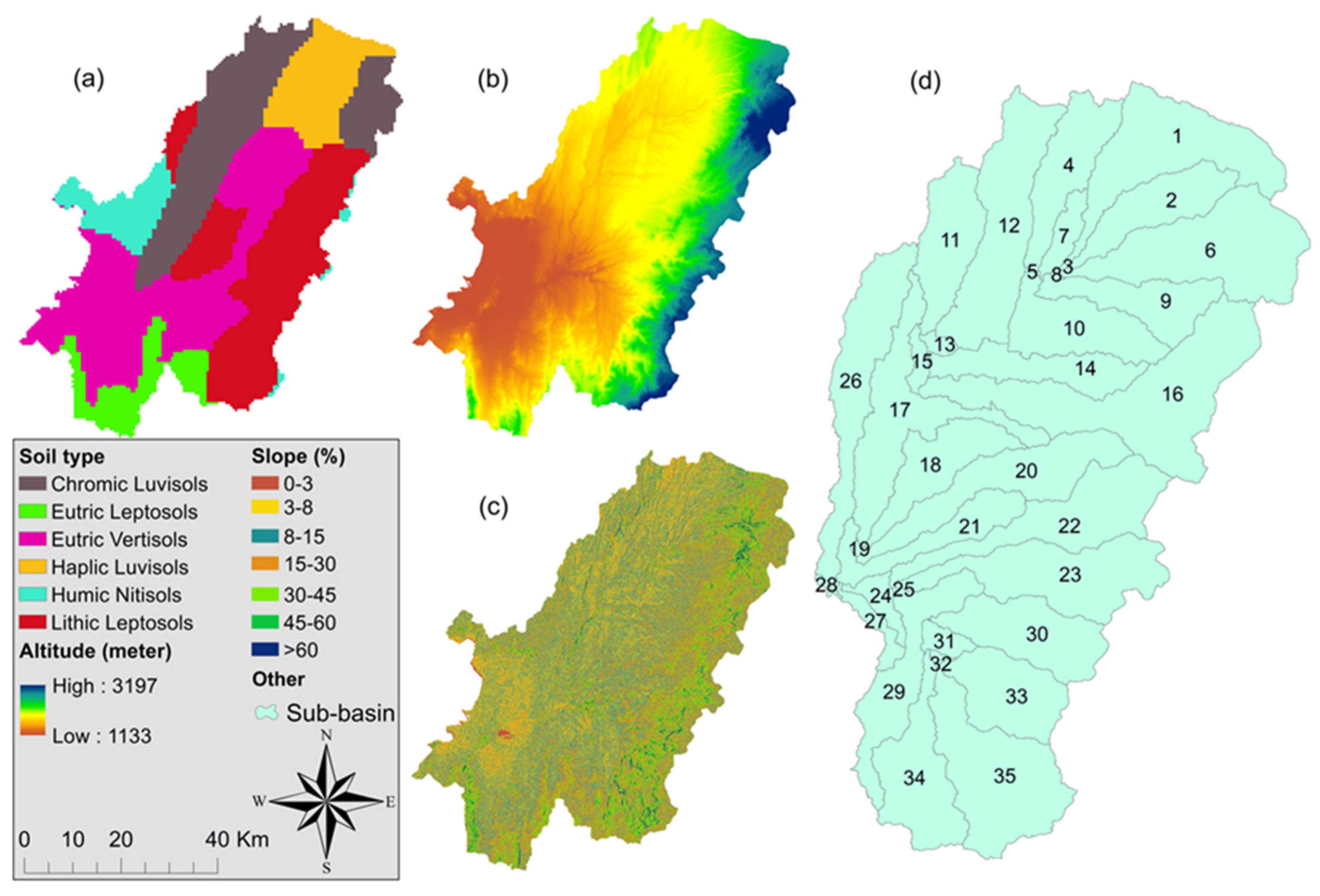
3.1. Biophysical Characteristics

More than 70% of the GRB is covered by three soil groups (Figure 2a): Eutric Vertisols (29%) characterized by a significant proportion of clay-sized particles and vetric property [63], Lithic Leptosols (25%) dominated in the eastern escarpment and have limited agricultural potential due to their shallow depth, low fertility and poor water-holding capacity [63], and Chromic Luvisols (22%) are soils with subsurface accumulation of high activity clays and high base saturation [64]. The altitude of the study area ranged from 1133 to 3197 m above sea level (a.s.l) (Figure 2b) and most (81%) of the basin exhibited gentle to moderate steep slopes (Figure 2c). The eastern part of the basin is characterized by longest and very steep slopes (having >45% slope), while the lower part is dominantly characterized by flat terrain (<3% slope). On the bases of topographic features, the study area was subdivided in to 35 sub-basins (Figure 2d).

3.2. Trends in Rainfall and Temperature

The trend analysis indicated that the observed mean annual rainfall experienced decreasing trend with a magnitude of about 13.4 mm/year from 1990 to 2005 (significantly) and 0.44 mm/year from 2006 to 2021 (insignificantly) (

Table 2. The Mann–Kendall and the Sen’s slope test results for rainfall and temperature.

Variable	Trend Test	Observed		RCP4.5		RCP8.5
		1990–2005	2006–2021	2021–2040	2041–2060	2021–2040	2041–2060
Rainfall	Z-Score	−1.39 ***	−0.22	−0.55	−0.49	−0.88	1.14
	Sen’s slope	−13.4	−0.44	−4.5	−6.4	−5.4	7.8
Minimum temperature	Z-Score	−0.05	0.88	2.63 *	1.46 ***	3.15 *	3.36 *
	Sen’s slope	−0.003	0.02	0.1	0.02	0.1	0.1
Maximum temperature	Z-Score	2.63 *	−0.44	2.17 **	0.81	2.95 *	1.72 **
	Sen’s slope	0.1	−0.01	0.04	0.02	0.04	0.03

*, **, *** means significant trend at alpha (α) = 0.01, 0.05, and 0.1, respectively.

). The observed mean annual maximum temperature showed a significant increasing trend, whereas minimum temperature declined insignificantly. Under RCP4.5, the projected mean annual rainfall showed a non-significant decreasing trend with a magnitude of about 4.5 and 6.4 mm/year (2021–2040 and 2041–2060, respectively). However, both mean annual minimum and maximum temperature showed statistically significant evidences of increasing trends (Table 2). Under high emission scenario (RCP8.5), the annual rainfall will decrease (at a rate of 5.4 mm/year during the near future) and increase (at a rate of 7.8 mm/year during the mid future) insignificantly, while both the annual minimum and maximum temperature will increase significantly. The results were consistent with the findings of previous studies [28,29,32,36]. The spatial pattern of projected mean annual rainfall and temperature were included in supplementary material (Figures S1 and S2).

3.3. Land Use Land Cover Dynamics

Nine LULC classes were identified, including waterbody, grasslands, forestlands, agriculture lands, bare land, settlements, agroforestry, shrublands and marshy area (Figure 3 and Figure 4). A detailed description of the LULC classification and change analysis can also be found in our recent study (Girma et al. [30]). In 1985, the largest land cover type was shrublands (24.3%) followed by forestlands (21.8%) and agriculture lands (19.8%) (Figure 3). However, agricultural lands, agroforestry and bare land showed increments and overturned the dominancy in 2003 and 2021 (Table S1). These unceasing expansion and trends will also be expected by 2035 and 2050 at the expense of forest, shrub and grasslands loss (Table S2). Moreover, the expansion of waterbodies (Figure 4), particularly along the shore side of Lake Abaya might be attributed to the displacement and lateral expansion of the lake’s water due to the increase in sediment load, resulting from soil erosion [65,66,67]. Rapid population growth, social instability, land policy, unproductive land and climate change were identified as the key driving forces of LULC changes in the area [33,68]. Land-use changes beyond land’s capability played a significant role in triggering land degradation [30]. To minimize these adverse consequences of land use change, it is recommended that adequate land use planning and management strategies must be implemented.

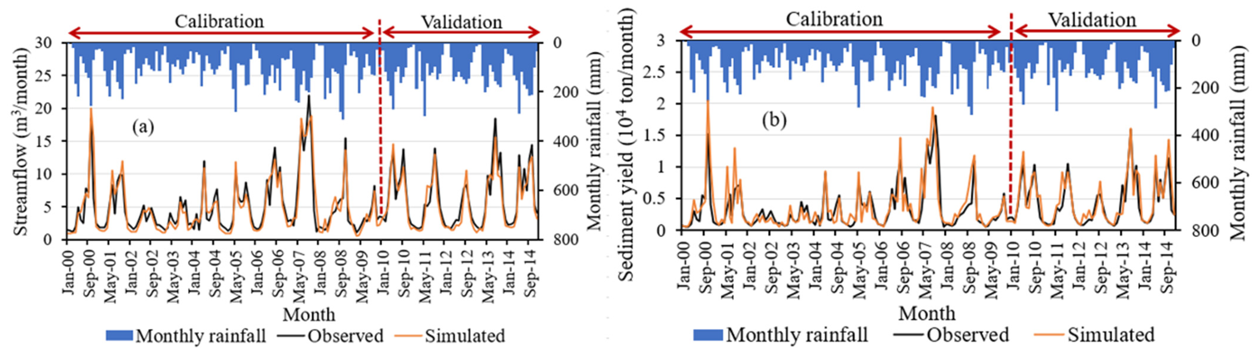
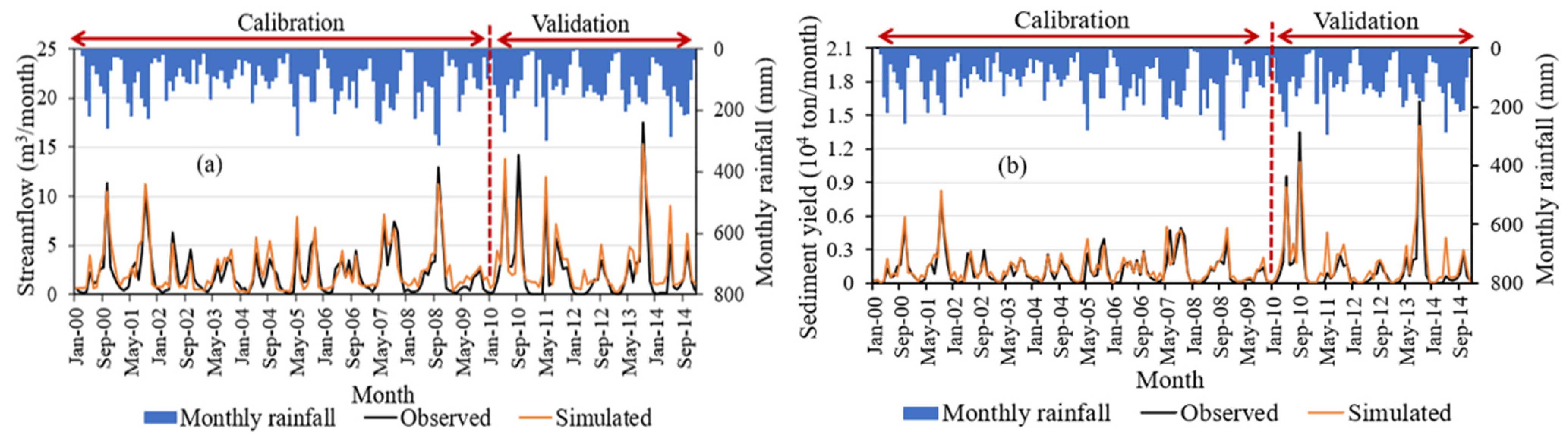
3.4. Sensitivity Analysis, Calibration and Validation

A total of fifteen parameters listed in

Table 3. Selected parameters, allowable range and fitted values for SWAT calibration.

Parameters	Description	Sensitivity			Allowable	Fitted
		t-Stat	p-Value	Rank	Range	Value
Streamflow
CN2	SCS runoff curve number	−21	0	1	35–98	0.15
ALPHA_BF	Baseflow alpha factor	−9.6	0	2	0–1	0.3
SOL_BD	Moist bulk density	−7.4	0	3	0.9–2.5	1.01
GW_DELAY	Groundwater delay	4.5	0.04	4	0–500	272
CH_K2	Effective hydraulic conductivity	3.8	0.1	5	−0.01–500	67
SOL_K	Saturated hydraulic conductivity	−3.7	0.16	6	0–2000	32
SOL_AWC	Available water capacity of the soil layer	1.6	0.34	7	0–1	0.16
Sediment
USLE_P	USLE support practice factor	−8.4	0	1	0–1	0.57
USLE_C	USLE cover factor	−5.8	0	2	0.001–0.5	0.05
CH_COV1	Channel erodibility factor	1.6	0.11	3	−0.05–0.6	0.03
SPCON	Linear factor for the channel sediment routing	1.3	0.25	4	0.0001–0.01	0.01
CH_EQN	Sediment routing method	1.2	0.27	5	0–4	3.0
SPEXP	Exponential factor for channel sediment routing	−0,68	0.49	6	1–2	1.2
CH_COV2	Channel cover factor	−0.64	0.51	7	−0.001–1	0.75
HRU_SLP	Average slope steepness	0.59	0.55	8	0–1	0.17

with very high to high sensitivity were selected. The sensitivity result showed the SCS runoff curve number (CN2) as a major key parameter with highest t-stat and lowest p-value (Table 3), while USLE_C and USLE_P are the two most important parameters for sediment calibration. The graphical representation in Figure 5 and Figure 6 showed that the magnitude and temporal variation of simulated and measured streamflow and sediment yield matched closely. As shown in

Table 4. Statistical indices for the SWAT model performance measure.

Model Simulation	Period	Aposto			Bedessa
		R2	NSE	PBIAS (%)	R2	NSE	PBIAS (%)
Streamflow	Calibration	0.89	0.80	−1.5	0.79	0.76	8.9
	Validation	0.81	0.75	−3.9	0.84	0.8	11.1
Sediment yield	Calibration	0.74	0.67	4.9	0.76	0.72	8.1
	Validation	0.8	0.76	3.6	0.84	0.77	13.8

, the R² values (R² > 0.74) were satisfactory, as indicated by the goodness-of-fit between the measured and simulated dataset. The NSE values indicated good model performance for stream flow and sediment yield simulation at both stations. The PBIAS showed slight underestimation at Aposto (streamflow) and overestimation at Bedessa. However, all the PBIAS values are less than ±15% indicating a good simulation [55]. Hence, all the statistical indices are in the acceptable range.

3.5. Estimation of Surface Runoff and Soil Loss

3.5.1. Impacts of Land Use Change on Surface Runoff and Soil Loss

The simulations that were driven from LULC change in the past indicated that the mean annual surface runoff increased by 15.3 mm (4.5%) and 23.4 mm (6.8%) during S2 and S3, respectively, compared to S1 (base period for past). Similarly, the sediment yield increased by 7.1 t/ha/year (28.8%) and 11.4 t/ha/year (46.2%) during S2 and S3, respectively. Despite lower precipitation, surface runoff and sediment yield were increased in the past. This could be attributed to the changes in LULC particularly the expansion of agricultural land at a rate of 3.23% per year at the expense of natural vegetation (deforestation at a rate of 2.4% per year) between 1985 and 2021 [30]. Moreover, significant changes were observed in settlement areas ranged between 1.5 and 9.5%.

Simulations driven by future modeled LULC and observed climate data (S7 and S8) showed an increase in surface runoff by 64.7 mm (17.8%) and 114.4 mm (31.5%), respectively, compared to S6 (baseline for future simulations). Likewise, the annual sediment yield increased by 5.1 t/ha/year (14.4%) and 8 t/ha/year (22.8%) during S7 and S8 compared to S6. Consequently, the predicted LULC change will lead to an increased surface runoff and sediment yield assuming a similar climate development as observed in S6. This could be due to the unceasing expansion of, for example, agriculture land (48.3%, 55%) and settlements (1.4%, 2%) by 2035 and 2050, respectively (Figure 3). The degradation of soil and vegetation may increase the area of impervious surface, lowers the infiltration capacity of the soil and increases the surface runoff [69,70]. The result revealed that land-use changes have a more positive synergy on surface runoff and sediment yield. The results were consistent with those in the previous studies [36,48].

3.5.2. Impacts of Climate Change on Surface Runoff and Soil Loss

Simulation obtained from climate change in the past (S4) depicted a decline in surface runoff by 3.9 mm (1.1%) and sediment yield by 0.9 t/ha/year (3.7%), as compared to S1. The near-term (S9) and mid-term (S10) simulations driven by future climate data (RCP4.5) and observed LULC (2021) decreased the surface runoff by 17.7 mm (4.9%) and 20.2 mm (5.6%), respectively, compared to S6. Likewise, the sediment yield will be reduced by 2.9 t/ha/year (8.3%) and 3.1 t/ha/year (8.9%) during the S9 and S10, respectively. Under RCP8.5, the surface runoff will decrease by 64.9 mm (17.9%) in the near-term (S11) and increase by 6.7 mm (1.9%) during the mid-term (S12), compared to S6. Correspondingly, the sediment yield will decrease by 4.6 t/ha/year (13%) in the S11 and increase by 1.7 t/ha/year (4.9%) in the S12. This might be related to the dynamic trends in climate variables (precipitation and temperature) in the future scenario period, as described in Table 2. The findings of decreasing surface runoff and sediment yield in the future projected scenarios were consistent with the results of other studies in the Ethiopian rift valley [36,45].

3.5.3. Combined Impacts of Land Use and Climate Change on Surface Runoff and Soil Loss

Under the combined effect of land use and climate change, there is high variation in annual surface runoff and sediment yield as compared to the individual effect. The result obtained from past simulation (S5 and S6) indicated that the annual runoff increased by 13.9 mm (4%) and 20.1 mm (5.9%), respectively, as compared to S1. Under these same scenarios, the sediment yield increased by 6 t/ha/year (24.2%) and 10.5 t/ha/year (42.7%), respectively, for S5 and S6. Urbanization and deforestation associated with land use change reduce the ability of land to absorb water, leading to increased surface runoff. Climate change can intensify this effect by causing more frequent and intense rainfall events, resulting in even higher rates of sediment yield. However, the combined effect of projected LULC (2035, 2050) and climate change indicated a decrease in surface runoff and sediment yield compared to S6.

Under RCP4.5, for example, the S13 (near-term) and S14 (mid-term) scenario showed a decrease in surface runoff by 10.3 mm (2.9%) and 13.6 mm (3.7%). Likewise, the sediment yield decreased by 2.4 t/ha/year (6.9%) and 2.6 t/ha/year (7.4%), respectively, in the S13 and S14. Under RCP8.5, S15 (near-term) showed a decrease in surface runoff and sediment yield by 41.5 mm (11.4%) and 3.1 t/ha/year (8.8%), respectively. Similarly, S17, S18 and S19 indicated a decrease in surface runoff and sediment yield. Thus, the percentage decrease in surface runoff ranged from 1.6% (S17) to 10.2% (S19). Similarly, the percentage decrease in sediment yield ranged from 1.1% (S18) to 5.4% (S19), whereas S16 and S20 showed an increase in surface runoff by 13.2 mm (3.6%) and 19.8 mm (5.5%), sediment yield by 2.5 t/ha/year (7.2%) and 3.96 mm (11.3%) into the future, respectively. This might be attributed to the expected increasing trends in the annual rainfall (7.8 mm/year) under the RCP8.5 scenario (Table 2). It is clearly evident that a little rise in annual precipitation is resulting in a higher surface flow. These findings were supported by previous studies on the impact of climate and LULC change on hydrological processes and sediment yield [36,71].

3.6. Identification of Soil Erosion Hotspots

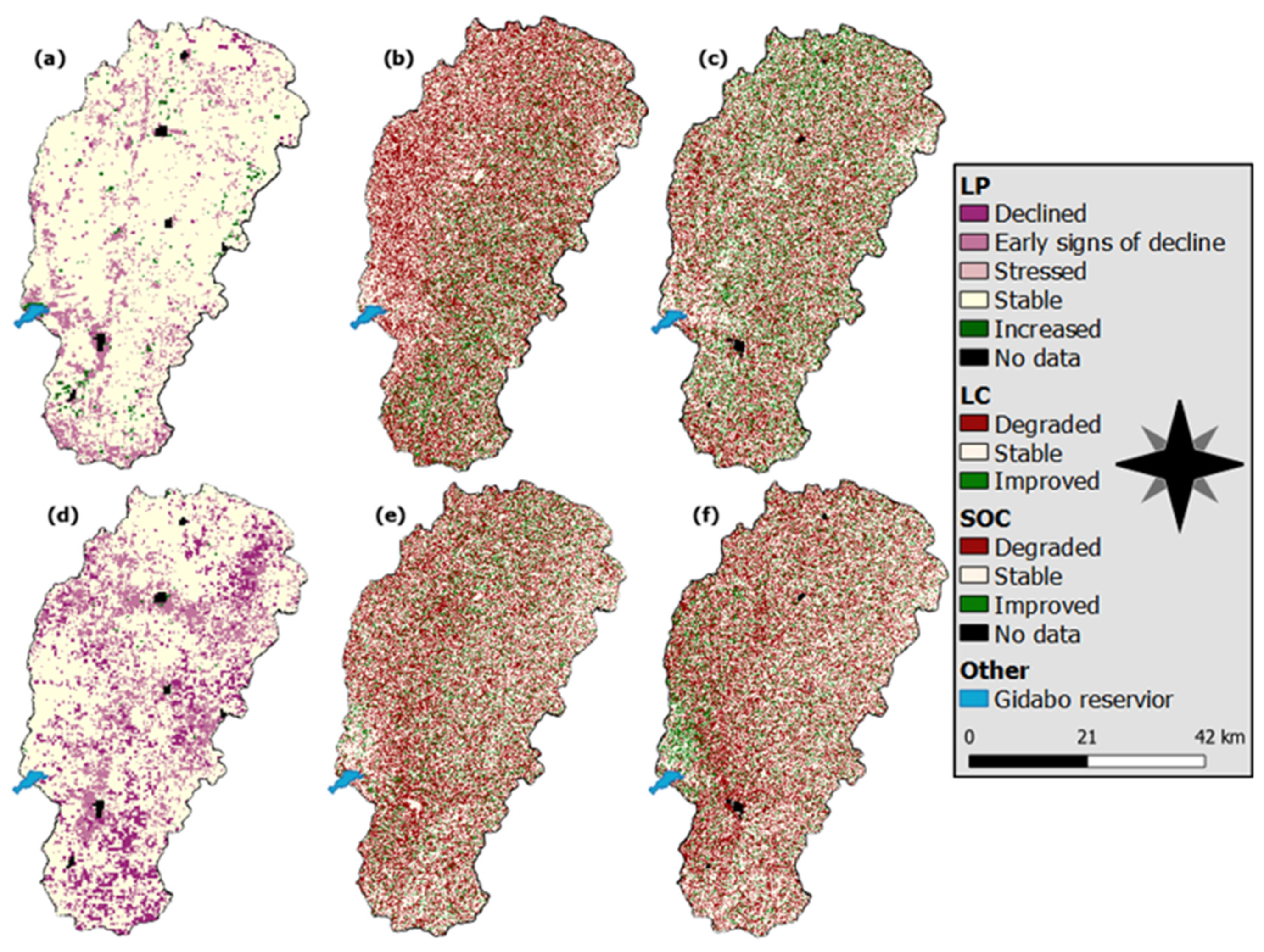
The identification of erosion hotspot areas is crucial for effective land and water resource management, as well as for developing targeted erosion control and mitigation strategies. Hence, the average annual soil loss of GRB was classified into five sediment severity classes (

Table 5. The percentage of erosion severity areas (Area%) in the past and future scenarios.

Severity Class	Description	Past		Near Future		Mid Future
		S1	S5	S13	S15	S18	S20
0–5	Low	4.9	4.9	0.7	0.7	0.7	0.6
5–10	Moderate	18.6	13.6	0.9	0.9	4.1	0.1
10–25	High	38.8	33.7	26.9	32.8	51.5	10.5
25–50	Very high	32.7	40.1	51.3	52	26.2	60.8
>50	Severe	5	7.7	20.2	13.6	17.5	28

). The classes were adapted from Dananto et al. [47]; Guduru and Jilo [38]. Table 5 indicated that most (>77%) of the study area experienced high to severe soil erosion rate in a given scenario. The past analysis depicted that a mean annual soil loss of 42.9 t/ha/year and 45.6 t/ha/year was accounted for in S1 and S5, respectively. Moreover, Figure 7 showed the spatial variability of mean annual soil loss at sub-basin scale under the different scenarios. The highest amount of soil loss was showed in the southern as well as in eastern part of the basin (Figure 7 and Figures S1 and S5), characterized by widespread steep slopes and more often, the southern part received the high amount of rainfall [39]. On the contrary, most of the sub-basins in the western and northern part experienced low to high soil loss. The results are consistent with Dananto et al. [47]; Adi et al. [48]; Guduru and Jilo [38].

Furthermore, the spatial variability of sediment yield was identified for future combined scenarios. The combined scenario analysis (Section 3.5.3) depicted the insignificant intra-variability within each RCP scenario. Hence, we used a combination of one future period (2021–2040, 2041–2060) correspondingly for each projected land use (LULC 2035, LULC 2050) under each RCP (2 LULC $\times$ 2 pathways $\times$ 1 climate $=$ 4). In this line, S13 and S15 as well as S18 and S20 were considered for near and mid future scenario, respectively. Thus, the near future average annual sediment yield varied between 28.25 t/ha/year and 29.57 t/ha/year (S13 and S15, respectively), while the mid future average annual sediment yield ranged from 30.71 t/ha/year to 43.5 t/ha/year (S18 and S20, respectively). Among the 35 sub-basins (Figure 7), sub-basins 6, 19, 25, 27, 29, 30, 33, 34 and 35 will generate the highest amount of surface runoff and sediment yield in to the future (S13, S15, S18 and S20); thus, they were categorized under critical sub-basins.

3.7. LDN Indicators

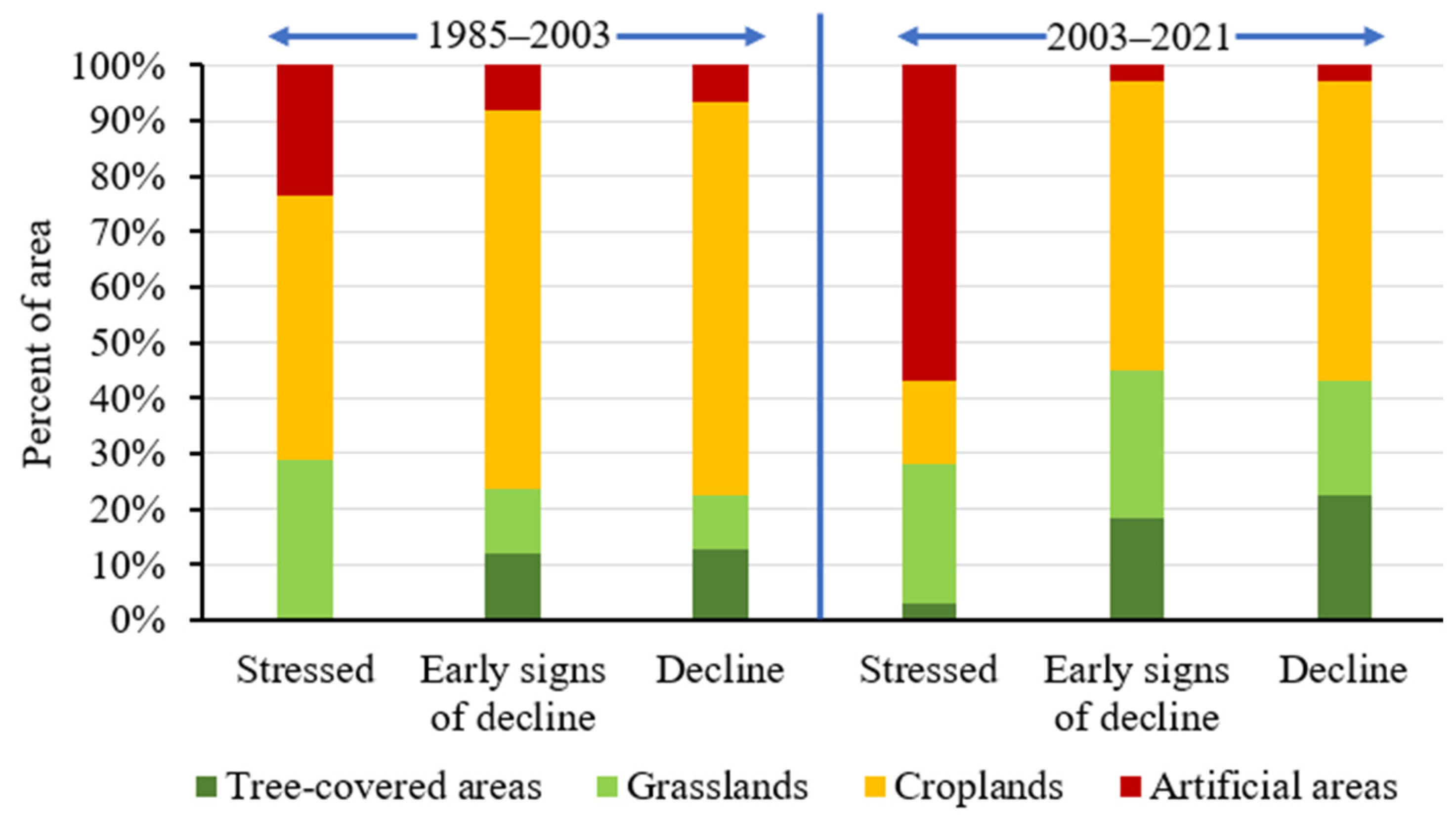
3.7.1. Land Productivity Dynamics

From 1985 to 2003, most (83.2%) of the study area was characterized under stable productivity class and smaller (1.6%) proportion of the study area showed improvements in productivity (Table S3). The LP trend showed early signs of decline in 13.2% of the area. Another 1.4% of the study area showed decline land productivity and insignificant proportion (0.01%) of the study area characterized as stressed. Based on the LP trend analysis applied between 2003 and 2021, 67% of the study area was marked as stable (Table S3). Furthermore, 18.4% and 14.1% of the study area were under early signs of decline and decline, respectively. Similar to the previous years, an insignificant proportion (0.03%) of the study area was characterized as stressed between 2005 and 2021.

The stress or pressure on land productivity varied with land use and land cover. For example, out of the total stressed area, 48% were found in croplands. Similarly, the largest share of early signs of decline (68%) and decline (71%) categories were contributed from croplands in 1985–2003 (Figure 8). Furthermore, the share of the area with early signs of decline (52%) and decline (53.8%) were higher in croplands from 2003 to 2021 (Figure 8), while around 57% of the stressed category were found in artificial areas between 2003 to 2021. From 1985–2003 to 2003–2021, the area where LP was improved and stable were reduced while the land area degraded were increased (Figure 9a,d, respectively).

3.7.2. Land Cover Degradation

The outputs for the land cover sub-indicator revealed that land area with stable land cover were dominant (52% and 47%) in both periods (1985–2003 and 2003–2021, respectively). Additionally, the degraded land cover was increased from 36% during the 1985–2003 to 42% during the 2003–2021 (Figure 9b,e). However, land area with improved land cover was slightly reduced from 12% during the 1985–2003 to 11% during the 2003–2021 (Table S3). The long-term LULC dynamics indicated that GRB experienced significant landscape alteration between 1985 and 2021 (Table S1). Croplands covering 20% of the study area (in 1985) experienced the highest relative expansion by 25% and 40% (in 2003 and 2021, respectively). Similarly, the spatial extent of agroforestry was increased from 13% to 15% and 20% over the study years. The other major rate of change was recorded in the residential areas from 1.5% to 9.5% between 1985–2003 and 2003–2021, respectively. This reflects the intensification of agricultural practice and urbanization activity in the GRB. Furthermore, the expansion of agroforestry was mainly attributed to cultural values and traditional beliefs in the study area [68].

3.7.3. Soil Organic Carbon Loss

Figure 9c,f showed the spatial distribution of SOC over the two periods (1985–2003 and 2003–2021, respectively). The results indicated that 13% and 12% of the study area showed improvement in SOC, 53% and 49% of the GRB displayed stable condition during 1985–2003 and 2003–2021, respectively (Table S3). In addition, it appeared that the percentage of degraded areas were increased from 35% in 1985–2003 to 39% in 2003–2021. This could be attributed to the significant conversion of forestlands (–1.16%, –4.23%), grasslands (−1.31%, −3.26%) and shrublands (−2.41%, −3.59%) to other land uses, mainly croplands (Table S3) and extractive nature of the farming practice. In line with this, Negasa et al. [72] and Okolo et al. [73] indicated that conversion of native forest to other land uses and the intensification of agricultural activities resulted in a significant decrease in the SOC stocks across Ethiopia.

3.7.4. Land Degraded Status

Combining all the three sub-indicators, 45% and 56% of the study area were under degraded status, 41% and 31% unchanged, 14% and 12% improved over the periods between 1985–2003 and 2003–2021, respectively (

Table 6. The extent of degraded, stable, and improved land according to the SDG 15.3.1 indicator.

Land Degradation Status	1985–2003 (% of Land)	2003–2021 (% of Land)
Stable	40.9	30.9
Improved	13.7	12.3
Degraded	44.6	56
No data	0.8	0.8

). From 1985–2003 to 2003–2021, the proportion of degraded land was increased by 26%, while stable and improved land areas were reduced by 25% and 9%, respectively. The expansion of degraded area might be attributed to the dynamic interplay of climate and LULC change. The high-risk degraded land was mainly located in areas dominated by croplands and bare land (Figure 10).

3.8. Sediment Yield under Soil Conservation Scenarios

The average annual sediment yield reduction (% reduction) with respect to the soil conservation practices was presented in

Table 7. Mean annual sediment reduction in soil conservation scenarios over the entire basin.

Conservation Scenarios	Sediment Yield (% Reduction) *
	S13	S15	S18	S20
Terracing	77.2	63.1	78.9	70.8
Contour farming	72	58.4	77.1	71
Filter strip	38.7	38.4	45.2	33.1
Stone/soil bund	79.8	67.9	81.1	76.2
Reforestation	67.9	55.7	70.4	63

* Compared to the corresponding “without SWC” scenario.

. The result revealed that soil/stone bund generated the lowest value of sediment yield (5.7–10.3 t/ha/year), then terracing (6.4–12.7 t/ha/year) and contour farming (7–12.6 t/ha/year), followed by reforestation (9.1–16.1 t/ha/year) and filter strip of 1 m (16.8–29.1 t/ha/year). Furthermore, Figure 11 shows the distribution of average sediment yield (t/ha/year) in critical sub-basins under the proposed conservation scenario. The analysis justified that soil conservation practices used in each scenario could significantly reduce the annual sediment yield. At the implementation of terracing, for example, there are no areas within the severe sediment yield category. Accordingly, 64.8% and 59.4% (Low), 21.6% and 27% (moderate), 13.6% (high to very high) were classified during S13 and S15, respectively. Likewise, 36.4% and 29.2% of the study area were accounted for low severity class during S18 and S20, respectively, while 51.9% and 47.2% were identified as moderate class. The remaining (11.7% and 23,6%) were grouped under high to very high class during S18 and S20, respectively. The results attained are comparable with the findings of previous studies in GRB [47,48]. Similarly, Lemma et al. [25], Gashaw et al. [60], Admas et al. [61], Leta et al. [74] quantified the significant contribution of the aforementioned conservation scenarios in different part of the country.

4. Discussion

4.1. Key Features and Variables

While there has been a significant decline in rainfall in the earlier past (1990–2005), the trend in the more recent years (2005–2021) was relatively stable in the GRB. The future projections under different emission scenarios (RCP4.5 and RCP8.5) indicated varying trends, with temperature increases being a consistent feature. This indicates that the basin is likely to experience warmer conditions in the future, which can have various implications for ecosystems, water resources and human activities. For example, rising temperatures will amplify the impact of droughts, reducing soil moisture availability and cropland productivity [75]. Since majority of the livelihoods were primarily dependent on subsistence rainfed agriculture [35], these trends could have significant effects on agricultural practices and might be the determinant factor for various socio-economic problems in the basin. These findings emphasize the need for robust climate monitoring and adaptation strategies to address the potential impacts of changing climate conditions on water resources, agriculture and overall environmental sustainability in the region.

The existing diverse range of LULC types reflects the complex nature of the landscape and its susceptibility to change. The results revealed significant shifts in land cover over the past several years (1985–2021). The “from–to” analysis in Tables S1 and S2 showed a substantial conversion of natural landscapes into cultivable areas and settlements. By 2035 and 2050, it is expected that agricultural lands, agroforestry and bare land will continue to expand at the expense of forest, shrub and grasslands. These projections are indicative of ongoing land use changes that could have far-reaching environmental and socio-economic consequences [76]. The increase in human population often leads to higher demands for land, particularly for agriculture and settlements [33]. Effective land-use planning and management are critical for achieving sustainable and resilient landscapes.

4.2. Land Degradation Pathways

The results of the simulations, which were driven by land use and climate change scenarios, provide valuable insights into the impacts on soil erosion and land degradation. Comparing baseline (S1 and S6) and land use change alone, the simulations indicated a substantial increase in surface runoff and sediment yield. Therefore, the study boldly underscored that land use change alone have a more positive synergy on surface runoff and soil loss. For example, the conversion of natural landscapes, such as forestlands, shrublands and grasslands into agriculture land and urban areas, including impervious surfaces like roads and buildings, reduced the land’s ability to absorb and retain water [69,70]. These lead to an increase in surface runoff while decreasing infiltration. Moreover, deforestation and clearing of natural vegetation leave the soil exposed to the erosive forces of water and leading to more water reaching the ground and contributing to runoff. Additionally, land-use changes can modify natural drainage patterns, leading to the concentration of runoff into specific areas. This might result in localized flooding and erosion.

The comparison between the baseline and climate change scenario showed decrease that might be attributed to a decrease in precipitation and an increase in temperature. The impacts of climate change on surface runoff and soil loss are interconnected. For example, Mana et al. [32] revealed the reduction in stream flow in the future due to the decrease in precipitation and an increase in evapotranspiration (associated with an increase in temperature). It has also been shown that there is a significant relationship between streamflow and sediment yield [45,48]. Thus, the result implies that the reduction in sediment yield (S9, S10 and S11) in the future period is associated with the reduction in streamflow, which is, in turn, linked with climate changes.

Despite increased impervious surface through increased settlement areas and bare land, lesser runoff and sediment yield were predicted in most of the combined future scenario compared to base period (S6). Additionally, the increments of runoff and sediment in these scenarios were lower compared to land use change alone (S7 and S8). This could be due to the offset of runoff and sediment reduction by climate change (i.e., lower precipitation and higher temperature projections) in the coupled climate and land-use change scenario. This indicates that climate change has greater contribution on hydrological process compared to land use.

Most of the critical sub-basins (28% of the total area) were characterized by shallow (Leptosols) and clay dominant soils (Vertisols), dominated by agriculture and grasslands, and very steep slopes. Moreover, the southern part of the GRB will receive high amount of rainfall under both RCPs (Figure S1). Regardless of differences in rainfall, surface runoff and soil erosion were much higher on croplands and grazing lands [77]. This is largely due to excessive tillage operations and intense grazing by livestock which lead to increased soil disruption and vulnerability to erosion. Moreover, high values of surface runoff were correlated with Vertisols owing to slow internal drainage and low infiltration capacity after getting wet [78,79]. On the contrary, sub-basins 4, 7, 8, 28 and 31, which represented 4.7% of the total area, were under low sediment severity class. These sub-basins were dominated by shrublands and forestlands with a slope ranged between 3 and 12%.

According to the LP dynamics, croplands accounted for 68.4% and 53% of the degraded area in 1985–2003 and 2003–2021, respectively. These areas are characterized by lower tree cover, unsustainable land management practices, accelerated carbon decomposition and erosion. In line with this, Degefa [80], Debelo et al. [81] and Hassen et al. [82] indicated that trend in agricultural productivity has declined over the last decades given that climate change, soil erosion, and poor soil and water conservation (SWC) practices were mentioned as the main drivers. This, in turn, resulted in increased demand for farm inputs (e.g., fertilizer, pesticides) and increased production costs. Moreover, studies identified that human and livestock population in regions of limited resources, unsustainable farming techniques, an insecure land tenure system, poverty and climate change as major drivers of LULC and land degradation [76,83,84,85]. As a result of the expansion of land degradation over time, agricultural productivity has decreased and worsened food insecurity and poverty in the GRB [35].

4.3. Enhancing Land Degradation Assessment

Soil erosion, as a key driver of land degradation, directly impacts soil quality and land productivity. Soil erosion assessment provides insights into erosion extent, severity and vulnerability of areas that may not be fully captured by the LDN sub-indicators alone. Moreover, soil erosion indicators can help to evaluate the success of land restoration activities, providing valuable feedback on the effectiveness of LDN interventions, and ultimately supports land management and conservation efforts. Therefore, the integration of soil erosion indicator into LDN assessments can complement the existing sub-indicators, allows for more comprehensive understanding of land degradation and restoration dynamics.

4.4. Potential Management Alternatives

Addressing these concerns, the study underscored the implementation of soil/stone bund, terracing, contour farming and reforestation practice. While these conservation practices had varying levels of effectiveness, they can significantly reduce the annual sediment yield and will help to achieve the LDN in the future. For example, soil/stone bund generated the lowest sediment yield values, indicating its high effectiveness in reducing soil erosion, while filter strip, although beneficial, was not as effective as the others. In line with this, Hassen et al. [86] revealed the positive correlation between soil conservation practice, agroecology and soil physicochemical properties in the GRB. Particularly, the traditional agroforestry system and plantation work has a significant contribution to soil fertility improvement and local communities’ livelihood [82,87]. Apparently, the integration of the proposed conservation scenarios with the traditional practice might reduce the soil erosion and also improve the LDN indicators, thereby reducing related degradations.

5. Conclusions

This study was conducted in the GRB, in an Ethiopian rift valley, to assess trends in land degradation and evaluate management alternatives. The study employed an integrated approach combining the SWAT model and the Trends.Earth. The GRB faces substantial landscape alteration and climatic variability, and significant challenges related to soil erosion and land degradation. Historical changes in LULC led to an increase in mean annual surface runoff and sediment yield despite lower precipitation. This increase is attributed to the expansion of agricultural land and deforestation, which reduced the land’s ability to absorb water and increased surface runoff. Future projection showed further increases in surface runoff and sediment yield due to the ongoing expansion of agriculture and settlements. Past simulations as well as future climate change scenarios under the RCP4.5 showed a decline in surface runoff and sediment yield, while under RCP8.5, results showed decreases in the near-term (2021–2040) and increases in the mid-term (2041–2060) in surface runoff and sediment yield. The interplay between land use and climate change led to varied outcomes, with some scenarios (e.g., S5 and S6) showed increases in surface runoff and sediment yield, indicating a synergy between land use change and climate change, while certain future scenarios (e.g., S13, S14, S15) showed decreases in surface runoff and sediment yield. The findings revealed that significant portion of the study area, particularly the southern and eastern parts of the basin, exhibited high to severe soil erosion rates. The LP dynamics indicated that the proportion of land categorized as stable were decreased, while areas displayed early signs of decline and decline were increased from 1985–2003 to 2003–2021. Concurrently, land-cover degradation and SOC loss was also increased. Overall, the proportion of degraded land expanded significantly emphasizing the need for sustainable land management practices to mitigate further degradation. The study evaluated various soil conservation practices in the context of sediment yield reduction, with soil/stone bund emerging as the most effective measure, followed by terracing, contour farming and reforestation. These practices exhibited the potential to significantly reduce annual sediment yield and are crucial for achieving LDN goals.

References

1. Sanz, M.J.; de Vente, J.; Chotte, J.L.; Bernoux, M.; Kust, G.; Ruiz, I.; Almagro, M.; Alloza, J.A.; Vallejo, R.; Castillo, V.; et al. Sustainable Land Management Contribution to Successful Land-Based Climate Change Adaptation and Mitigation: A Report of the Science-Policy Interface; United Nations Convention to Combat Desertification (UNCCD): Bonn, Germany, 2017. [Google Scholar]
2. UNCCD. Land Degradation Neutrality Transformative Projects and Programs: Operational Guidance for Country Support; United Nations Convention to Combat Desertification (UNCCD): Bonn, Germany, 2019. [Google Scholar]
3. Orr, B.J.; Cowie, A.L.; Castillo Sanchez, V.M.; Chasek, P.; Crossman, N.D.; Erlewein, A.; Louwagie, G.; Maron, M.; Metternicht, G.I.; Minelli, S.; et al. Scientific Conceptual Framework for Land Degradation Neutrality; A Report of the Science-Policy Interface; United Nations Convention to Combat Desertification (UNCCD): Bonn, Germany, 2017. [Google Scholar]
4. IPBES. The IPBES Assessment Report on Land Degradation and Restoration; Montanarella, L., Scholes, R., Brainich, A., Eds.; IPBES: Bonn, Germany, 2018. [Google Scholar]
5. Verburg, P.H.; Metternicht, G.; Allen, C.; Debonne, N.; Akhtar-Schuster, M.; da Cunha, M.I.; Karim, Z.; Pilon, A.; Raja, O.; Santivañez, M.S.; et al. Creating an Enabling Environment for Land Degradation Neutrality: And Its Potential Contribution to Enhancing Well-Being, Livelihoods and the Environment; United Nations Convention to Combat Desertification (UNCCD): Bonn, Germany, 2019. [Google Scholar]
6. Akça, E.; Büyük, G.; İnan, M.; Kırpık, M. Sustainable Management of Land Degradation through Legume-Based Cropping System. In Advances in Legumes for Sustainable Intensification; Academic Press: Cambridge, MA, USA, 2022. [Google Scholar]
7. Pricope, N.G.; Daldegan, G.A.; Zvoleff, A.; Mwenda, K.M.; Noon, M.; Lopez-Carr, D. Operationalizing an Integrative Socio-Ecological Framework in Support of Global Monitoring of Land Degradation. Land Degrad. Dev. 2023, 34, 109–124. [Google Scholar] [CrossRef]
8. UNCCD. The Global Land Outlook, East Africa Thematic Report; United Nations Convention to Combat Desertification (UNCCD): Bonn, Germany, 2019. [Google Scholar]
9. Shitu, D. Cause of Land Degradation and Rehabilitation Practices in Case of Amba Sidist Western Ethiopia. Am. J. Chem. Pharm. 2022, 1, 18–25. [Google Scholar] [CrossRef]
10. Moges, S.A.; Gebregiorgis, A.S. Climate Vulnerability on the Water Resources Systems and Potential Adaptation Approaches in East Africa: The Case of Ethiopia. In Climate Vulnerability: Understanding and Addressing Threats to Essential Resources; Elsevier: Amsterdam, The Netherlands, 2013; Volume 5. [Google Scholar]
11. Kirui, O.K.; Mirzabaev, A.; von Braun, J. Assessment of Land Degradation ‘on the Ground’ and from ‘Above’. SN Appl. Sci. 2021, 3, 318. [Google Scholar] [CrossRef]
12. García, C.L.; Teich, I.; Gonzalez-Roglich, M.; Kindgard, A.F.; Ravelo, A.C.; Liniger, H. Land Degradation Assessment in the Argentinean Puna: Comparing Expert Knowledge with Satellite-Derived Information. Environ. Sci. Policy 2019, 91, 70–80. [Google Scholar] [CrossRef]
13. Nzuza, P.; Ramoelo, A.; Odindi, J.; Kahinda, J.M.; Madonsela, S. Predicting Land Degradation Using Sentinel-2 and Environmental Variables in the Lepellane Catchment of the Greater Sekhukhune District, South Africa. Phys. Chem. Earth 2021, 124, 102931. [Google Scholar] [CrossRef]
14. Gibbs, H.K.; Salmon, J.M. Mapping the World’s Degraded Lands. Appl. Geogr. 2015, 57, 12–21. [Google Scholar] [CrossRef]
15. Yang, L.; Zhao, G.; Mu, X.; Lan, Z.; Jiao, J.; An, S.; Wu, Y.; Miping, P. Integrated Assessments of Land Degradation on the Qinghai-Tibet Plateau. Ecol. Indic. 2023, 147, 109945. [Google Scholar] [CrossRef]
16. Feng, S.; Zhao, W.; Zhan, T.; Yan, Y.; Pereira, P. Land Degradation Neutrality: A Review of Progress and Perspectives. Ecol. Indic. 2022, 144, 109530. [Google Scholar] [CrossRef]
17. Sims, N.C.; England, J.R.; Newnham, G.J.; Alexander, S.; Green, C.; Minelli, S.; Held, A. Developing Good Practice Guidance for Estimating Land Degradation in the Context of the United Nations Sustainable Development Goals. Environ. Sci. Policy 2019, 92, 349–355. [Google Scholar] [CrossRef]
18. Schillaci, C.; Jones, A.; Vieira, D.; Munafò, M.; Montanarella, L. Evaluation of the United Nations Sustainable Development Goal 15.3.1 Indicator of Land Degradation in the European Union. Land Degrad. Dev. 2023, 34, 250–268. [Google Scholar] [CrossRef]
19. Zhao, L.; Jia, K.; Liu, X.; Li, J.; Xia, M. Assessment of Land Degradation in Inner Mongolia between 2000 and 2020 Based on Remote Sensing Data. Geogr. Sustain. 2023, 4, 100–111. [Google Scholar] [CrossRef]
20. Giuliani, G.; Chatenoux, B.; Benvenuti, A.; Lacroix, P.; Santoro, M.; Mazzetti, P. Monitoring Land Degradation at National Level Using Satellite Earth Observation Time-Series Data to Support SDG15–Exploring the Potential of Data Cube. Big Earth Data 2020, 4, 3–22. [Google Scholar] [CrossRef]
21. Borrelli, P.; Van Oost, K.; Meusburger, K.; Alewell, C.; Lugato, E.; Panagos, P. A Step towards a Holistic Assessment of Soil Degradation in Europe: Coupling on-Site Erosion with Sediment Transfer and Carbon Fluxes. Environ. Res. 2018, 161, 291–298. [Google Scholar] [CrossRef]
22. Tsymbarovich, P.; Kust, G.; Kumani, M.; Golosov, V.; Andreeva, O. Soil Erosion: An Important Indicator for the Assessment of Land Degradation Neutrality in Russia. Int. Soil Water Conserv. Res. 2020, 8, 418–429. [Google Scholar] [CrossRef]
23. Ricci, G.F.; De Girolamo, A.M.; Abdelwahab, O.M.M.; Gentile, F. Identifying Sediment Source Areas in a Mediterranean Watershed Using the SWAT Model. Land Degrad. Dev. 2018, 29, 1233–1248. [Google Scholar] [CrossRef]
24. Gao, X.; Yan, C.; Wang, Y.; Zhao, X.; Zhao, Y.; Sun, M.; Peng, S. Attribution Analysis of Climatic and Multiple Anthropogenic Causes of Runoff Change in the Loess Plateau—A Case-Study of the Jing River Basin. Land Degrad. Dev. 2020, 31, 1622–1640. [Google Scholar] [CrossRef]
25. Lemma, H.; Frankl, A.; van Griensven, A.; Poesen, J.; Adgo, E.; Nyssen, J. Identifying Erosion Hotspots in Lake Tana Basin from a Multisite Soil and Water Assessment Tool Validation: Opportunity for Land Managers. Land Degrad. Dev. 2019, 30, 1449–1467. [Google Scholar] [CrossRef]
26. dos Santos, F.M.; de Souza Pelinson, N.; de Oliveira, R.P.; Di Lollo, J.A. Using the SWAT Model to Identify Erosion Prone Areas and to Estimate Soil Loss and Sediment Transport in Mogi Guaçu River Basin in Sao Paulo State, Brazil. Catena 2023, 222, 106872. [Google Scholar] [CrossRef]
27. Mechal, A.; Wagner, T.; Birk, S. Recharge Variability and Sensitivity to Climate: The Example of Gidabo River Basin, Main Ethiopian Rift. J. Hydrol. Reg. Stud. 2015, 4, 644–660. [Google Scholar] [CrossRef]
28. Belihu, M.; Abate, B.; Tekleab, S.; Bewket, W. Hydro-Meteorological Trends in the Gidabo Catchment of the Rift Valley Lakes Basin of Ethiopia. Phys. Chem. Earth Parts A/B/C 2018, 104, 84–101. [Google Scholar] [CrossRef]
29. Alehu, B.A.; Desta, H.B.; Daba, B.I. Assessment of Climate Change Impact on Hydro-Climatic Variables and Its Trends over Gidabo Watershed. Model. Earth Syst. Environ. 2021, 8, 3769–3791. [Google Scholar] [CrossRef]
30. Girma, R.; Fürst, C.; Moges, A. Land Use Land Cover Change Modeling by Integrating Artificial Neural Network with Cellular Automata-Markov Chain Model in Gidabo River Basin, Main Ethiopian Rift. Environ. Chall. 2022, 6, 100419. [Google Scholar] [CrossRef]
31. Worako, A.W.; Haile, A.T.; Taye, M.T. Implication of Bias Correction on Climate Change Impact Projection of Surface Water Resources in the Gidabo Sub-Basin, Southern Ethiopia. J. Water Clim. Chang. 2022, 13, 2070–2088. [Google Scholar] [CrossRef]
32. Mana, T.T.; Abebe, B.W. Assessment of Hydro-Meteorological Regimes of Gidabo River Basin under Representative Concentration Pathway Scenarios. Model. Earth Syst. Environ. 2023, 9, 473–491. [Google Scholar] [CrossRef]
33. WoldeYohannes, A.; Cotter, M.; Kelboro, G.; Dessalegn, W. Land Use and Land Cover Changes and Their Effects on the Landscape of Abaya-Chamo Basin, Southern Ethiopia. Land 2018, 7, 2. [Google Scholar] [CrossRef]
34. Belihu, M.; Tekleab, S.; Abate, B.; Bewket, W. Hydrologic Response to Land Use Land Cover Change in the Upper Gidabo Watershed, Rift Valley Lakes Basin, Ethiopia. HydroResearch 2020, 3, 85–94. [Google Scholar] [CrossRef]
35. Wolde, Z.; Wei, W.; Likessa, D.; Omari, R.; Ketema, H. Understanding the Impact of Land Use and Land Cover Change on Water–Energy–Food Nexus in the Gidabo Watershed, East African Rift Valley. Nat. Resour. Res. 2021, 30, 2687–2702. [Google Scholar] [CrossRef]
36. Aragaw, H.M.; Mishra, S.K.; Goel, M.K. Responses of Water Balance Component to Land Use/Land Cover and Climate Change Using Geospatial and Hydrologic Modeling in the Gidabo Watershed, Ethiopia. Geocarto Int. 2022, 37, 17119–17144. [Google Scholar] [CrossRef]
37. Serur, A.B.; Adi, K.A. Multi-Site Calibration of Hydrological Model and the Response of Water Balance Components to Land Use Land Cover Change in a Rift Valley Lake Basin in Ethiopia. Sci. Afr. 2022, 15, e01093. [Google Scholar] [CrossRef]
38. Guduru, J.U.; Jilo, N.B. Assessment of Rainfall-Induced Soil Erosion Rate and Severity Analysis for Prioritization of Conservation Measures Using RUSLE and Multi-Criteria Evaluations Technique at Gidabo Watershed, Rift Valley Basin, Ethiopia. Ecohydrol. Hydrobiol. 2023, 23, 30–47. [Google Scholar] [CrossRef]
39. Girma, R.; Fürst, C.; Moges, A. Performance Evaluation of CORDEX-Africa Regional Climate Models in Simulating Climate Variables over Ethiopian Main Rift Valley: Evidence from Gidabo River Basin for Impact Modeling Studies. Dyn. Atmos. Oceans 2022, 9, 101317. [Google Scholar] [CrossRef]
40. Dibaba, W.T.; Miegel, K.; Demissie, T.A. Evaluation of the CORDEX Regional Climate Models Performance in Simulating Climate Conditions of Two Catchments in Upper Blue Nile Basin. Dyn. Atmos. Oceans 2019, 87, 101104. [Google Scholar] [CrossRef]
41. Demissie, T.A.; Sime, C.H. Assessment of the Performance of CORDEX Regional Climate Models in Simulating Rainfall and Air Temperature over Southwest Ethiopia. Heliyon 2021, 7, e07791. [Google Scholar] [CrossRef] [PubMed]
42. Gao, P.; Li, P.; Zhao, B.; Xu, R.; Zhao, G.; Sun, W.; Mu, X. Use of Double Mass Curves in Hydrologic Benefit Evaluations. Hydrol. Process. 2017, 31, 4639–4646. [Google Scholar] [CrossRef]
43. IPCC. Sections. In Climate Change 2023: Synthesis Report. Contribution of Working Groups I, II and III to the Sixth Assessment Report of the Intergovernmental Panel on Climate Change; Core Writing Team; Lee, H., Romero, J., Eds.; IPCC: Geneva, Switzerland, 2023. [Google Scholar]
44. FAO & IIASA Harmonized World Soil Database Version 2.0; FAO: Rome, Italy; IIASA: Laxenburg, Austria, 2023. [CrossRef]
45. Gadissa, T.; Nyadawa, M.; Behulu, F.; Mutua, B. The Effect of Climate Change on Loss of Lake Volume: Case of Sedimentation in Central Rift Valley Basin, Ethiopia. Hydrology 2018, 5, 67. [Google Scholar] [CrossRef]
46. Assfaw, A.T. Modeling Impact of Land Use Dynamics on Hydrology and Sedimentation of Megech Dam Watershed, Ethiopia. Sci. World J. 2020, 2020, 6530278. [Google Scholar] [CrossRef]
47. Dananto, M.; Aga, A.O.; Yohannes, P.; Shura, L. Assessing the Water-Resources Potential and Soil Erosion Hotspot Areas for Sustainable Land Management in the Gidabo Watershed, Rift Valley Lake Basin of Ethiopia. Sustainability 2022, 14, 5262. [Google Scholar] [CrossRef]
48. Adi, K.A.; Serur, A.B.; Meskele, D.Y. Sediment Yield Responses to Land Use Land Cover Change and Developing Best Management Practices in the Upper Gidabo Dam Watershed. Sustain. Water Resour. Manag. 2023, 9, 68. [Google Scholar] [CrossRef]
49. Toma, M.B.; Belete, M.D.; Ulsido, M.D. Hydrological Components and Sediment Yield Response to Land Use Land Cover Change in The Ajora-Woybo Watershed of Omo-Gibe Basin, Ethiopia. Air Soil Water Res. 2023, 16, 11786221221150186. [Google Scholar] [CrossRef]
50. Neitsch, S.L.; Arnold, J.G.; Kiniry, J.R.; Williams, J.R. Soil & Water Assessment Tool Theoretical Documentation Version 2009; Texas Water Resources Institute: College Station, TX, USA, 2011. [Google Scholar] [CrossRef]
51. Arnold, J.G.; Moriasi, D.N.; Gassman, P.W.; Abbaspour, K.C.; White, M.J.; Srinivasan, R.; Santhi, C.; Harmel, R.D.; Van Griensven, A.; Van Liew, M.W.; et al. SWAT: Model Use, Calibration, and Validation. Trans. ASABE 2012, 55, 1491–1508. [Google Scholar] [CrossRef]
52. Church, M. Bed Material Transport and the Morphology of Alluvial River Channels. Annu. Rev. Earth Planet. Sci. 2006, 34, 325–354. [Google Scholar] [CrossRef]
53. Aga, A.O.; Chane, B.; Melesse, A.M. Soil Erosion Modelling and Risk Assessment in Data Scarce Rift Valley Lake Regions, Ethiopia. Water 2018, 10, 1684. [Google Scholar] [CrossRef]
54. Lenhart, T.; Eckhardt, K.; Fohrer, N.; Frede, H.G. Comparison of Two Different Approaches of Sensitivity Analysis. Phys. Chem. Earth 2002, 27, 645–654. [Google Scholar] [CrossRef]
55. Moriasi, D.N.; Zeckoski, R.W.; Arnold, J.G.; Baffaut, C.B.; Malone, R.W.; Daggupati, P.; Guzman, J.A.; Saraswat, D.; Yuan, Y.; Wilson, B.W.; et al. Hydrologic and Water Quality Models: Key Calibration and Validation Topics. Trans. ASABE 2015, 58, 1609–1618. [Google Scholar] [CrossRef]
56. Abraham, T.; Liu, Y.; Tekleab, S.; Hartmann, A. Prediction at Ungauged Catchments through Parameter Optimization and Uncertainty Estimation to Quantify the Regional Water Balance of the Ethiopian Rift Valley Lake Basin. Hydrology 2022, 9, 150. [Google Scholar] [CrossRef]
57. Teich, I.; Harari, N.; Caza, P.; Henao-Henao, J.P.; Lopez, J.C.; Raviolo, E.; Díaz-González, A.M.; González, H.; Bastidas, S.; Morales-Opazo, C.; et al. An Interactive System to Map Land Degradation and Inform Decision-making to Achieve Land Degradation Neutrality via Convergence of Evidence across Scales: A Case Study in Ecuador. Land Degrad. Dev. 2023, 34, 4475–4487. [Google Scholar] [CrossRef]
58. Trends.Earth. Trends Earth User Guide 2.1.8. Conservation International. 2023. Available online: http://trends.earth (accessed on 20 June 2023).
59. Qiu, J.; Shen, Z.; Hou, X.; Xie, H.; Leng, G. Evaluating the Performance of Conservation Practices under Climate Change Scenarios in the Miyun Reservoir Watershed, China. Ecol. Eng. 2020, 143, 105700. [Google Scholar] [CrossRef]
60. Gashaw, T.; Worqlul, A.W.; Dile, Y.T.; Addisu, S.; Bantider, A.; Zeleke, G. Evaluating Potential Impacts of Land Management Practices on Soil Erosion in the Gilgel Abay Watershed, Upper Blue Nile Basin. Heliyon 2020, 6, e04777. [Google Scholar] [CrossRef]
61. Admas, B.F.; Gashaw, T.; Adem, A.A.; Worqlul, A.W.; Dile, Y.T.; Molla, E. Identification of Soil Erosion Hot-Spot Areas for Prioritization of Conservation Measures Using the SWAT Model in Ribb Watershed, Ethiopia. Resour. Environ. Sustain. 2022, 8, 100059. [Google Scholar] [CrossRef]
62. Hurni, H.; Berhe, W.A.; Chadhokar, P.; Daniel, D.; Gete, Z.; Grunder, M.; Kassaye, G. Soil and Water Conservation in Ethiopia: Guidelines for Development Agents; Ministry of Agriculture (MoA): Addis Ababa, Ethiopia, 2016. [Google Scholar]
63. FAO-UNESCO. Soils Map of the World: Revised Legend; FAO-UNESCO: Rome, Italy, 1988. [Google Scholar]
64. Nachtergaele, F.O.; van Velthuizen, H.; Verelst, L.; Wiberg, D.; Batjes, N.H.; Dijkshoorn, J.A.; van Engelen, V.W.P.; Fischer, G.; Jones, A.; Montanarella, L.; et al. Harmonized World Soil Database (Version 1.2); FAO and ISRIC: Rome, Italy, 2012. [Google Scholar]
65. Zekarias, T.; Govindu, V.; Kebede, Y.; Gelaw, A. Geospatial Analysis of Wetland Dynamics on Lake Abaya-Chamo, The Main Rift Valley of Ethiopia. Heliyon 2021, 7, e07943. [Google Scholar] [CrossRef]
66. Dadi Belete, M.; Diekkrüger, B.; Roehrig, J. Characterization of Water Level Variability of the Main Ethiopian Rift Valley Lakes. Hydrology 2015, 3, 1. [Google Scholar] [CrossRef]
67. Schütt, B.; Thiemann, S.; Wenclawiak, B. Deposition of Modern Fluvio-Lacustrine Sediments in Lake Abaya, South Ethiopia—A Case Study from the Delta Areas of Bilate River and Gidabo River, Northern Basin. Geomorphol. NF 2005, 138, 131–151. [Google Scholar]
68. Hassen, G.; Bantider, A.; Legesse, A.; Maimbo, M.; Likissa, D. Land Use and Land Cover Change for Resilient Environment and Sustainable Development in the Ethiopian Rift Valley Region. Ochr. Srodowiska I Zasobow Nat. 2021, 32, 24–41. [Google Scholar] [CrossRef]
69. Nyatuame, M.; Amekudzi, L.K.; Agodzo, S.K. Assessing the Land Use/Land Cover and Climate Change Impact on Water Balance on Tordzie Watershed. Remote Sens. Appl. 2020, 20, 100381. [Google Scholar] [CrossRef]
70. Tan, X.; Liu, S.; Tian, Y.; Zhou, Z.; Wang, Y.; Jiang, J.; Shi, H. Impacts of Climate Change and Land Use/Cover Change on Regional Hydrological Processes: Case of the Guangdong-Hong Kong-Macao Greater Bay Area. Front. Environ. Sci. 2022, 9, 688. [Google Scholar] [CrossRef]
71. Giri, S.; Arbab, N.N.; Lathrop, R.G. Assessing the Potential Impacts of Climate and Land Use Change on Water Fluxes and Sediment Transport in a Loosely Coupled System. J. Hydrol. 2019, 577, 123955. [Google Scholar] [CrossRef]
72. Negasa, T.; Ketema, H.; Legesse, A.; Sisay, M.; Temesgen, H. Variation in Soil Properties under Different Land Use Types Managed by Smallholder Farmers along the Toposequence in Southern Ethiopia. Geoderma 2017, 290, 40–50. [Google Scholar] [CrossRef]
73. Okolo, C.C.; Gebresamuel, G.; Retta, A.N.; Zenebe, A.; Haile, M. Advances in Quantifying Soil Organic Carbon under Different Land Uses in Ethiopia: A Review and Synthesis. Bull. Natl. Res. Cent. 2019, 43, 99. [Google Scholar] [CrossRef]
74. Leta, M.K.; Waseem, M.; Rehman, K.; Tränckner, J. Sediment Yield Estimation and Evaluating the Best Management Practices in Nashe Watershed, Blue Nile Basin, Ethiopia. Environ. Monit. Assess. 2023, 195, 716. [Google Scholar] [CrossRef]
75. Shigute, M.; Alamirew, T.; Abebe, A.; Ndehedehe, C.E.; Kassahun, H.T. Analysis of Rainfall and Temperature Variability for Agricultural Water Management in the Upper Genale River Basin, Ethiopia. Sci. Afr. 2023, 20, e01635. [Google Scholar] [CrossRef]
76. Mekuria, W.; Diyasa, M.; Tengberg, A.; Haileslassie, A. Effects of Long-Term Land Use and Land Cover Changes on Ecosystem Service Values: An Example from the Central Rift Valley, Ethiopia. Land 2021, 10, 1373. [Google Scholar] [CrossRef]
77. Ebabu, K.; Taye, G.; Tsunekawa, A.; Haregeweyn, N.; Adgo, E.; Tsubo, M.; Fenta, A.A.; Meshesha, D.T.; Sultan, D.; Aklog, D.; et al. Land Use, Management and Climate Effects on Runoff and Soil Loss Responses in the Highlands of Ethiopia. J. Environ. Manag. 2023, 326, 116707. [Google Scholar] [CrossRef] [PubMed]
78. Tibebe, D.; Bewket, W. Surface Runoff and Soil Erosion Estimation Using the SWAT Model in the Keleta Watershed, Ethiopia. Land Degrad. Dev. 2011, 22, 551–564. [Google Scholar] [CrossRef]
79. Garg, K.K.; Anantha, K.H.; Dixit, S.; Nune, R.; Venkataradha, A.; Wable, P.; Budama, N.; Singh, R. Impact of Raised Beds on Surface Runoff and Soil Loss in Alfisols and Vertisols. Catena 2022, 211, 105972. [Google Scholar] [CrossRef]
80. Degefa, S. Home Garden Agroforestry Practices in the Gedeo Zone, Ethiopia: A Sustainable Land Management System for Socio-Ecological Benefits. In Socio-Ecological Production Landscapes and Seascapes (SEPLS) in Africa; United Nations University: Tokyo, Japan, 2007. [Google Scholar]
81. Regassa Debelo, A.; Legesse, A.; Milstein, T.; Orkaydo, O.O. “Tree Is Life”: The Rising of Dualism and the Declining of Mutualism among the Gedeo of Southern Ethiopia. Front. Commun. 2017, 2, 7. [Google Scholar] [CrossRef]
82. Hassen, G.; Bantider, A.; Legesse, A.; Maimbo, M. Assessment of Design and Constraints of Physical Soil and Water Conservation Structures in Respect to the Standard in the Case of Gidabo Sub-Basin, Ethiopia. Cogent Food Agric. 2021, 7, 1855818. [Google Scholar] [CrossRef]
83. Meshesha, D.T.; Tsunekawa, A.; Tsubo, M. Continuing Land Degradation: Cause-Effect in Ethiopia’s Central Rift Valley. Land Degrad. Dev. 2012, 23, 130–143. [Google Scholar] [CrossRef]
84. Desta, H.; Fetene, A. Land-Use and Land-Cover Change in Lake Ziway Watershed of the Ethiopian Central Rift Valley Region and Its Environmental Impacts. Land Use Policy 2020, 96, 104682. [Google Scholar] [CrossRef]
85. Mesfin, D.; Simane, B.; Belay, A.; Recha, J.W.; Taddese, H. Woodland Cover Change in the Central Rift Valley of Ethiopia. Forests 2020, 11, 916. [Google Scholar] [CrossRef]
86. Hassen, G.; Bantider, A.; Legesse, A.; Maimbo, M. The Effect of Soil and Water Conservation Structures on the Soil Physical and Chemical Properties in the Gidabo River Sub-Basin, Ethiopian Rift Valley. Int. J. Environ. Sci. Dev. 2021, 12, 363–371. [Google Scholar] [CrossRef]
87. Temesgen, H.; Wu, W.; Legesse, A.; Yirsaw, E.; Bekele, B. Landscape-Based Upstream-Downstream Prevalence of Land-Use/Cover Change Drivers in Southeastern Rift Escarpment of Ethiopia. Environ. Monit. Assess. 2018, 190, 166. [Google Scholar] [CrossRef] [PubMed]
Figure 1. Location of the Gidabo river basin.
Land 12 01809 g001
Figure 2. (a) Major soil groups, (b) altitude, (c) slope classes and (d) sub-basin in the GRB.
Land 12 01809 g002
Figure 3. The relative proportion of each land use.
Land 12 01809 g003
Figure 4. Past (1985, 2003, 2021) and future (2035, 2030) LULC maps.
Land 12 01809 g004
Figure 5. Monthly streamflow (a) and sediment yield (b) hydrograph during calibration and validation period at Aposto gauging station.
Land 12 01809 g005
Figure 6. Monthly streamflow (a) and sediment yield (b) hydrograph during calibration and validation period at Bedessa gauging station.
Land 12 01809 g006
Figure 7. The spatial pattern of sediment yield at the given scenario.
Land 12 01809 g007
Figure 8. The distribution of LP sub-indicator across the different land use and land cover types.
Land 12 01809 g008
Figure 9. Land degradation sub-indicators LP (a,d), LC (b,e), SOC (c,f) between 1985–2003 and 2003–2021, respectively.
Land 12 01809 g009
Figure 10. Land degradation neutrality indicator map between 1985–2003 (a) to 2003–2021 (b) in the Gidabo river basin.
Land 12 01809 g010
Figure 11. Comparison of the conservation practices in critical sub-basins under a given scenario.
Land 12 01809 g011