Article

Effects of Land Cover Changes on Shallow Landslide Susceptibility Using SlideforMAP Software (Mt. Nerone, Italy)

1
Department of Agriculture, Food, Environment and Forestry, University of Florence, Via San Bonaventura 13, 50145 Firenze, Italy
2
Department of Agricultural, Food and Environmental Sciences, Marche Polytechnic University, Via Brecce Bianche 10, 60131 Ancona, Italy
3
Nuoro Forestry School, Department of Agricolture, University of Sassari, Viale Italia 39, 07100 Sassari, Italy
4
CoSci LLC, Shorewood, WI 53211, USA
5
School of Agricultural, Forest and Food Sciences, Bern University of Applied Sciences, Länggasse 85, 3052 Zollikofen, Switzerland
*
Author to whom correspondence should be addressed.
Land 2024, 13(10), 1575; https://doi.org/10.3390/land13101575
Submission received: 9 August 2024 / Revised: 17 September 2024 / Accepted: 24 September 2024 / Published: 27 September 2024

Abstract

:
Land cover changes in mountainous areas due to silvo-pastoral abandonment can affect soil stability, especially on steep slopes. In addition, the increase in rainfall intensity in recent decades requires re-assessing landslide susceptibility and vegetation management for soil protection. This study was carried out using the software SlideforMAP in the Mt. Nerone massif (central Italy) to assess (i) the effects of land cover changes on slope stability over the past 70 years (1954–2021) and (ii) the role of actual vegetation cover during intense rainfall events. The study area has undergone a significant change in vegetation cover over the years, with a reduction in mainly pastures (−80%) and croplands (−22%) land cover classes in favor of broadleaf forests (+64%). We simulated twelve scenarios, combining land cover conditions and rainfall intensities, and analyzed the landslide failure probability results. Vegetation cover significantly increased the slope stability, up to three to four times compared to the unvegetated areas (29%, 68%, and 89%, respectively, in the no cover, 1954, and 2021 scenarios). The current land cover provided protection against landslide susceptibility, even during extreme rainfall events, for different return periods. The 30-year return period was a critical condition for a significant stability reduction. In addition, forest species provide different mitigation effects due to their root system features. The results showed that species with deep root systems, such as oaks, provide more effective slope stability than other species, such as pines. This study helps to quantify the mitigation effects of vegetation cover and suggests that physically based probabilistic models can be used at the regional scale to detect the areas prone to failure and the triggering of rainfall-induced shallow landslides. This approach can be important in land planning and management to mitigate risks in mountainous regions.

1. Introduction

Natural hazards arise from the interaction of various physical predisposing factors, including topography, soil characteristics and vegetation, and triggering events such as intense rainfall. In mountainous regions, environmental features such as steep slopes, fractured rock formations, and complex topography [1,2] significantly contribute to the occurrence of shallow landslides, particularly during heavy precipitation events [3].
For centuries, the mountainous landscapes of the central Apennines have been shaped by human activities such as grazing, timber, firewood, and charcoal production [4]. The establishment of human settlements in these mountainous areas frequently led to deforestation or modifications to the natural slope, primarily through activities such as road construction, footpath development, and terrace building. These alterations in land use and the resulting changes in hillslope morphology are associated with an increased frequency of landslides [5,6,7]. However, social changes since the post-war period have induced the abandonment of mountainous areas, leading to rapid changes in land use [8,9]. After World War II and until the 1980s, a national reforestation program for slope stabilization in this area led to the planting of 760,000 hectares of mainly conifer tree species. These land cover changes over the last 67 years have caused a simplification of the mountainous landscape matrix but also reduced land management and maintenance after disturbances [10,11,12,13,14].
A significant body of research indicates that forested mountainous regions exhibit a lower susceptibility to shallow landslides compared to non-forested slopes (e.g., [15,16]); thus, vegetation represents a natural protection against natural hazards such as erosion and landslides. Many researchers have made significant contributions to understanding the effects of forests on shallow landslides [17,18,19,20,21]. Liu et al. [22] investigated the stabilizing effects of Lolium perenne on slopes, highlighting the importance of roots and soil cover for soil particle retention. Mehtab et al. [23] demonstrated that tree stem diameter significantly influences root distribution and tensile strength in Cunninghamia lanceolata forests, with larger diameters correlating with increased root reinforcement and enhanced soil shear resistance.
The mechanism by which vegetation enhances slope stability involves a complex interplay of mechanical and hydrological processes. We can identify three main mechanisms of root reinforcement, as highlighted by recent studies on root mechanics and hydrological modeling [24,25,26]: (i) roots contribute to an increase in soil stiffness, making the soil less prone to deformation. As roots grow in the soil matrix, they create a natural reinforcement structure, enhancing the soil’s overall resistance to shear forces and stiffness. This process works by improving the load-bearing capacity of the soil, distributing external forces more evenly and limiting soil deformation. Moreover, improved soil structure, supported by root systems and microbial activity, further stabilizes the soil, reducing susceptibility to erosion and landslides [18,27]; (ii) roots are highly effective under both tensile and compressive stresses. Under tension, roots resist being pulled out of the soil in the upper and lateral side of a landslide, while under compression, they offer resistance to being crushed or bent at the toe of the unstable slope [24,28]. The tensile strength of roots, especially that of the larger roots of plants or trees, is particularly important in slope stabilization [29]. Even smaller roots contribute to this process, as they collectively form a network that holds soil particles and enhances soil aggregation [27,30]; (iii) finally, one of the most critical mechanisms by which roots prevent shallow landslides is by crossing potential shear planes within the soil. Roots that penetrate across the shear plane or are growing in the substratum act as natural anchors, resisting the slide movement by binding the layers together. This is the most efficient way to prevent localized failures, reducing the risk of soil detachment and displacement [28,31,32,33,34].
In addition to the mechanism described, canopy tree interception, stem flow, and soil porosity significantly influence the hydrological balance. Canopy interception captures rainfall, reducing the net amount that reaches the soil surface and slowing soil saturation, which is a critical factor in triggering shallow landslides [35].
Developing slope stability models for assessing landslide susceptibility is an essential research topic for risk analyses [36,37]. Refs. [38,39] analyzed some common slope stability models used in the literature and suggested criteria for their selection. Improvements to the data accessibility and analysis details required by these models make them usable at different scales and in diverse contexts. The choice of a specific model depends mainly on the scope of the analysis, the spatial scale, and the available data. For example, probabilistic models are preferable for analysis at catchment or regional scales, because they consider spatial variability and uncertainty of the required input parameters. However, when assessing the mitigation effect of vegetation against shallow landslides, it is advisable to use slope stability models that explicitly consider vegetation cover and root reinforcement [14,31,40,41,42,43].
In this study, we analyzed the landslide susceptibility of a mountainous area and the relationship with land cover changes over 67 years. The analysis involved the reconstruction of scenarios based on different land cover conditions and rainfall intensity, aiming to (i) model the effects of vegetation on slope stability by comparing past scenarios with the most current ones, and (ii) evaluate the current stabilizing effect of forest cover by considering precipitation with different return periods.

2. Materials and Methods

2.1. Study Area

The study area is in the central Italian Apennines, in the northern Marche region bordering Umbria and Tuscany, where Mt. Nerone is one of the highest peaks at 1525 m a.s.l. (Figure 1). The study area, approximately 5600 hectares, belongs to the Metauro River catchment. Meteorological data for climate classification were retrieved from the E- OBS 27.0e grid for 1950–2020 time intervals [44]. According to the Rivas–Martinez bioclimatic classification system [45], the study area has a temperate oceanic climate (sub Mediterranean variant), an upper meso temperate thermotype, and a low humid ambrotype. The mean annual temperature is 12 °C, and the mean annual cumulative precipitation is 1164 mm, occurring mainly from autumn to early spring, with periods of water deficit in late July and August. Geological substrates are predominantly limestones and dolomites [46], with a widespread karst system [47]. The Regional Soils Service database identifies six different soil types for this area, according to the FAO World Reference Base for Soil Resources classification system. The most representative soil classes are Mollic Leptosols (69% of the area), Calcari-Epileptic Phaeozems (22%), and Eutric Cambisols (4%), which show a fine silty texture with coarse fragments. Soil thickness ranges from 25 to 150 cm. The study area is mainly covered by pastures, shrublands, mixed broadleaf forests (Quercus cerris and Quercus pubescens; Ostrya carpinifolia and Fraxinus ornus), a few Pinus nigra plantations, and, above 1000 m a.s.l., pure Fagus sylvatica forests. Broadleaf forests were generally managed as coppices and now are mainly stored coppices or undergoing conversion to high forests.

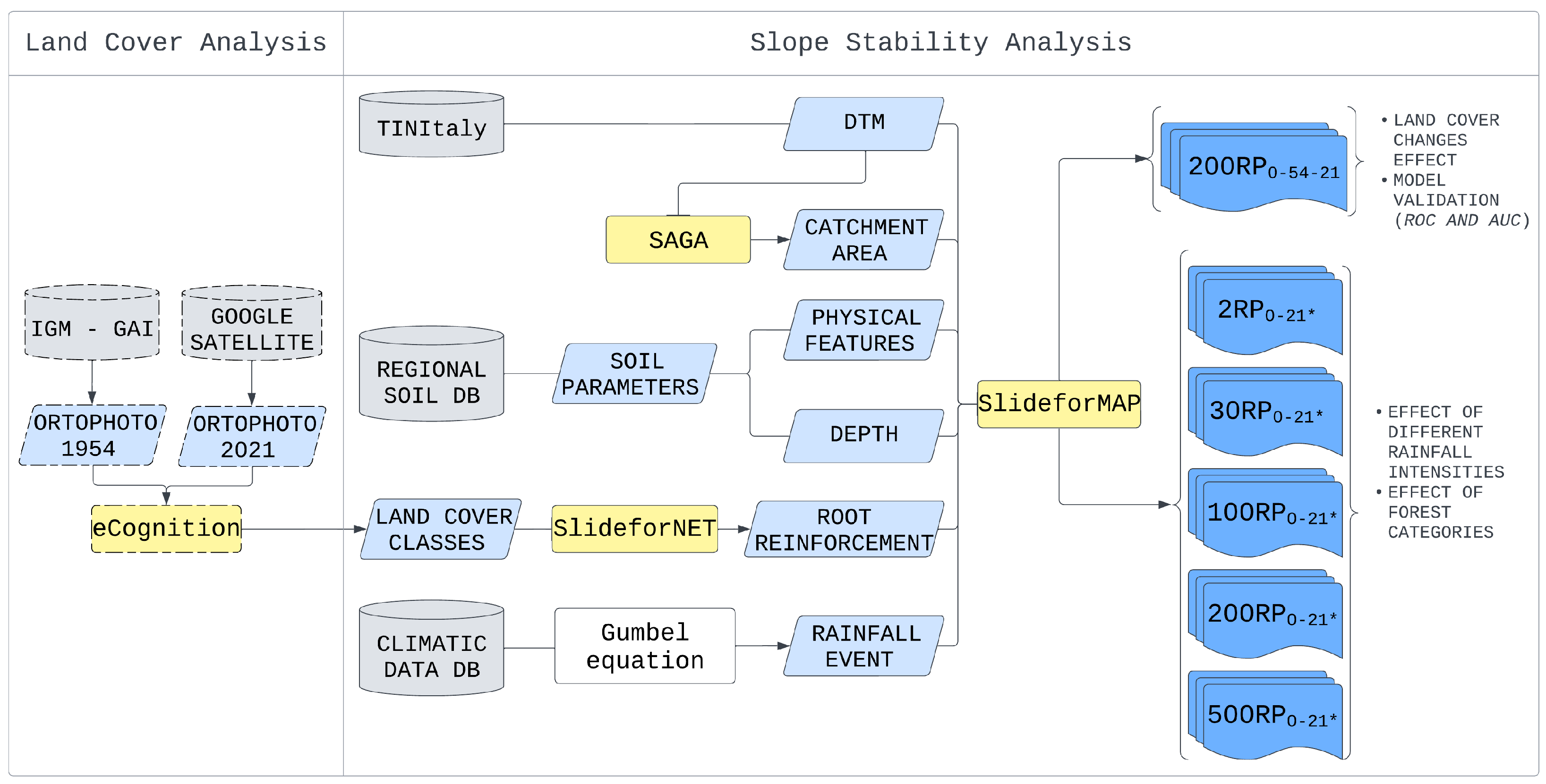
2.2. Workflow for Assessing Shallow Landslide Susceptibility

The workflow for simulating landslide susceptibility using the SlideforMAP model was developed through a series of methodical steps, summarized as follows:
  • Initial susceptibility assessment: We first calculated the susceptibility to shallow landslides without considering the contributions from vegetation cover. This analysis utilized rainfall depths corresponding to return periods of 2, 30, 100, 200, and 500 years.
  • Vegetation contribution assessment (1954) using land cover classes: We assessed the susceptibility to shallow landslides by incorporating the contributions of land cover classes as found in 1954, alongside a rainfall depth representative of a 200-year return period.
  • Vegetation contribution assessment (2021) using land cover classes: We evaluated the susceptibility to shallow landslides, including land cover classes from 2021, alongside a rainfall depth representative of a 200-year return period.
  • Vegetation contribution assessment (2021) using forest categories: We evaluated the susceptibility to shallow landslides, including forest categories data from 2021, and considering rainfall depths for return periods of 2, 30, 100, 200, and 500 years.
By combining the results from steps 1, 2, 3, and 4, we generated a total of twelve distinct scenarios (see Table 1). The scenarios are designated using the RP (return period) and land cover classification, represented as 200 RP 0 , 200 RP 54 , and 200 RP 21 . In this notation, the subscript 0 indicates no vegetation, 54 corresponds to vegetation cover as observed in 1954, and 21 represents vegetation cover in 2021, an asterisk corresponds to the forest categories instead of land cover classes. Figure 2 illustrates the data processing and preparation steps required for the simulations. To the right of the figure, the scenarios outlined in Table 1 are represented schematically, providing a clear visual representation of the analyzed conditions.
The comparative study between 1954 and 2021 aerial images focused on analyzing changes in broad land cover classes, specifically broadleaf and coniferous vegetation, rather than detailed forest categories and distribution. This approach was necessary due to the limited information available on the forest types and volumes in the 1954 aerial imagery, making it possible to effectively track and quantify the changes in land cover that occurred between the two time periods, despite the constraints of the historical data. This methodology allowed for a meaningful comparison of landscape-level transformations over the 67-year interval, even without the ability to differentiate more granular forest characteristics. Cross-comparisons between the no-cover scenario ( 200 RP 0 ) and the scenarios with vegetation ( 200 RP 54 and 200 RP 21 ) facilitated the assessment of how vegetation cover influences the probability of failure and the stability of slopes within the study area.
On the other hand, to evaluate the effectiveness of actual land cover in maintaining slope stability, we analyzed 2021 forest categories alongside rainfall events categorized by different return periods: 2 RP 21 *, 30 RP 21 *, 100 RP 21 *, 200 RP 21 , and 500 RP 21 . Each forest category was compared against its corresponding no-cover scenario ( 2 RP 0 , 30 RP 0 , 100 RP 0 , 200 RP 0 , and 500 RP 0 ) .

2.3. Land Cover Data and Analysis

For the classification of land cover classes in 1954, the aerial photos were sourced from the Italian Military Geographic Institute (IGMI), while satellite images from ©Google Earth were utilized for 2021. The 1954 IGMI aerial photos underwent orthorectification using contemporary satellite images and a 10 m resolution digital terrain model (DTM) as reference data [48]. The geometric correction of the 1954 IGMI images was performed using the PCI Geomatica software 2012, applying 50 control points per image, resulting in a mean root mean square error (RMSE) of 16–19 m. Land cover classification for both the 1954 IGMI images and the 2021 satellite images was conducted using a semi-automatic object-based approach. This method integrated automatic segmentation through eCognition Developer software 64 v8.9 (scale factor 100, color factor 0.5) with on-screen photo interpretation of segmented polygons [8,49]. Manual classification of the polygons followed the Corine classification system, categorizing nine land cover classes (Table 2): cropland (cr), tree groves (tg), unvegetated areas (un), pasture lands (ps), other woodland areas(wl), broadleaf forest (bf), conifer forest (cf), urban areas (ua), and roads and paths (rt). To validate the classification data, 300 random points were visually classified, yielding an overall classification accuracy ranging from 0.79 to 0.91, with a K coefficient between 70.3 and 77.1.
We obtained the change and persistence for each land cover class through a land cover transition matrix. Moreover, we analyzed the land cover patterns in 1954 and 2021 by quantifying diversity land cover metrics with Shannon evenness and Simpson indices, using the QGIS LecoS plugin [52].
Finally, the broadleaf and coniferous land cover classes were subsequently categorized into specific ‘forest categories’ (Table 2) according to the official databases established in 2001, including the regional forest Inventory [53], and the current forest management plan of the Mt. Nerone area [54]. The broadleaf forests were classified into five categories: holm oak (ho), downy oak (do), hop hornbeam–manna ash (hm), beech (be), and turkey oak (to), while coniferous forests were designated as black pine (bp) (Table 2).

2.4. Rainfall and Soil Data Collection

Rainfall heights were obtained from the Regional Meteo Information System (http://app.protezionecivile.marche.it/sol/indexjs.sol?lang=it, accessed on 20 October 2022). We used data series recorded from 1952 to the present from rain gauges located in the town of Piobbico, north of the study area, to calculate the rainfall height for a 1 h duration and different return periods through the Gumbel equation. The return periods were chosen based on the regional guidelines [55] for determining hydraulic hazard zones along streams and rivers, corresponding to 30 (30RP), 100 (100RP), 200 (200RP), and 500 (500RP) years. Additionally, we used a return period of 2 years (2RP) to consider the most frequent low-intensity rainfalls.
Six soil classes were identified following the Regional Soil Observatory (http://suoli.regione.marche.it/ServiziInformativi/Cartografia.aspx, accessed on 20 October 2022) and according to the Soil Classification System (USCS): from coarse-grained soils, with gravel well-graded (GW) and sand-silt mixtures (SM), to fine-grained soils with silt and low liquid limit clay (ML and CL) and silt and high liquid limit clay (MH and CH). The dataset and maps used for the rainfall scenarios and SlideforMAP simulation are freely available and reusable.

2.5. The SlideforMAP Slope Stability Model

For slope stability analysis, we used SlideforMAP, a 3D-physical-based probabilistic finite slope model based on limit equilibrium analysis [43]. SlideforMAP produces a raster file indicating slope failure probability values, which, along with outputs such as root reinforcement types, soil pore water pressure, and passive earth pressure, facilitates a comprehensive understanding of failure probabilities. This model is particularly effective for large forested areas, as is the case of the Mt. Nerone study area.
As a probabilistic model, SlideforMAP generates a substantial spatial distribution of hypothetical landslides within the study area, assessing the stability of each by integrating both deterministic and probabilistic parameters. Deterministic parameters include vegetation and soil hydrological characteristics, while probabilistic parameters encompass the location of hypothetical landslides, their area, soil cohesion, internal friction angle, pressure angle, and soil depth. A critical feature of SlideforMAP is its module designed to quantify the contribution of root reinforcement to the stability of vegetated slopes, considering both basal and lateral root reinforcement, as defined by Cohen and Schwarz [26]. Maximum lateral root reinforcement values were derived from the SlideforNET (SlideforNET (https://www.ecorisq.org/slidefor-net-en, accessed on 15 March 2023)) web application by simulating forest composition and structure, including dominant tree species, stem density, and average diameter at 130 cm height. Basal root reinforcement was subsequently calculated in SlideforMAP as a function of soil depth, employing a gamma distribution function with shape and scale coefficients provided by SlideforNET for each forest category.
Root reinforcement values for broadleaf and coniferous land cover classes were assigned based on the most prevalent species: hornbeam–manna ash for broadleaf forests and black pine for coniferous forests (Table 2). For the more detailed 2021 map, specific root reinforcement values were assigned to each subcategory of broadleaf and coniferous forests (Table 2). Root reinforcement values for cropland and grassland were taken from existing literature due to their unavailability in the SlideforNET database. In the absence of a defined value for “other wooded areas”, we assigned a general root reinforcement value of 3 kN/m, assuming these areas consist of mixed stands. Urban areas and roads and paths were excluded from the analysis.
The soil parameters incorporated in SlideforMAP included porosity (47% ± 6), field capacity (31% ± 10), friction angle (31° ± 3.63), cohesion (0 kPa), and hydraulic conductivity (5184 m/day). These parameters were calibrated using a 2-year return period scenario reflective of actual forest characteristics, assuming a low probability of failure. Multiple simulations were conducted to adjust the hydraulic conductivity, ensuring that less than 10% of the area exhibited a calculated landslide probability of less than 10%.
The resulting failure probability values were categorized into six classes: F10 for values between 0 and 10%; F20 for values between 10 and 20%; F40 for values between 20 and 40%; F60 for values between 40 and 60%; F80 for values between 60 and 80%; and F100 for values between 80 and 100%.

2.6. Slope Stability Model Validation

The Italian landslide inventory (IFFI (https://www.progettoiffi.isprambiente.it/, accessed on 9 August 2024), ISPRA [56]) identifies this area as having a significant susceptibility to landslides, mainly classified as rotational–translational movements. To evaluate the performance of the SlideforMAP model, we conducted a receiver operating characteristic (ROC) and area under the curve (AUC) analysis by comparing the IFFI dataset with the failure probability estimated by SlideforMAP. In a GIS environment, we selected random points within and outside the IFFI landslide areas, ensuring one point per hectare. We then assigned the failure probability value estimated for the 200 RP 54 scenario to each point and classified it as true-positive, false-positive, or false-negative. For instance, we considered a true-positive point within the IFFI landslide area if the failure probability was greater than 1%. We repeated this process ten times following the same criteria, and we calculated the AUC for each iteration.

3. Results and Discussion

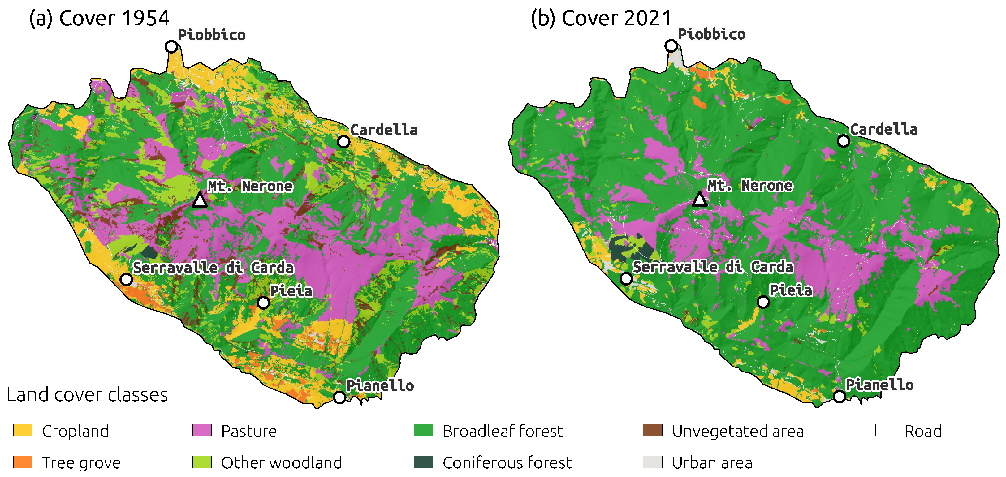
3.1. Land Cover Changes (1954–2021)

Over the past 70 years (1954–2021), land use has changed considerably, causing evident shifts in land cover classes and a marked reduction in landscape diversity (Figure 3). These observations are confirmed by the decreasing values of both Shannon evenness (0.68 to 0.39) and Simpson (0.71 to 0.41) diversity indices, as reported for most of the Apennines [8]. This process occurred in most Italian mountainous areas following the depopulation of the marginal regions and the consequent abandonment of traditional agro-pastoral activities [57]. This abandonment induced rapid secondary succession dynamics and the expansion of broadleaf forests, increasing their relative cover share by 64% (Table 1), corresponding to a landscape change of 29% (about 1634 ha). Conversely, land cover categories like pastures (−435.08 ha), croplands (−419.28 ha), non-vegetated areas (−201.08 ha), and other woodlands (−571.45 ha) decreased remarkably (Table 3). In particular, croplands and other woodlands almost completely disappeared, decreasing by 80% and 94%, respectively. Coniferous forests showed the highest relative area increase (224%), even if their absolute value is negligible (26 ha, 0.46% of the landscape share).

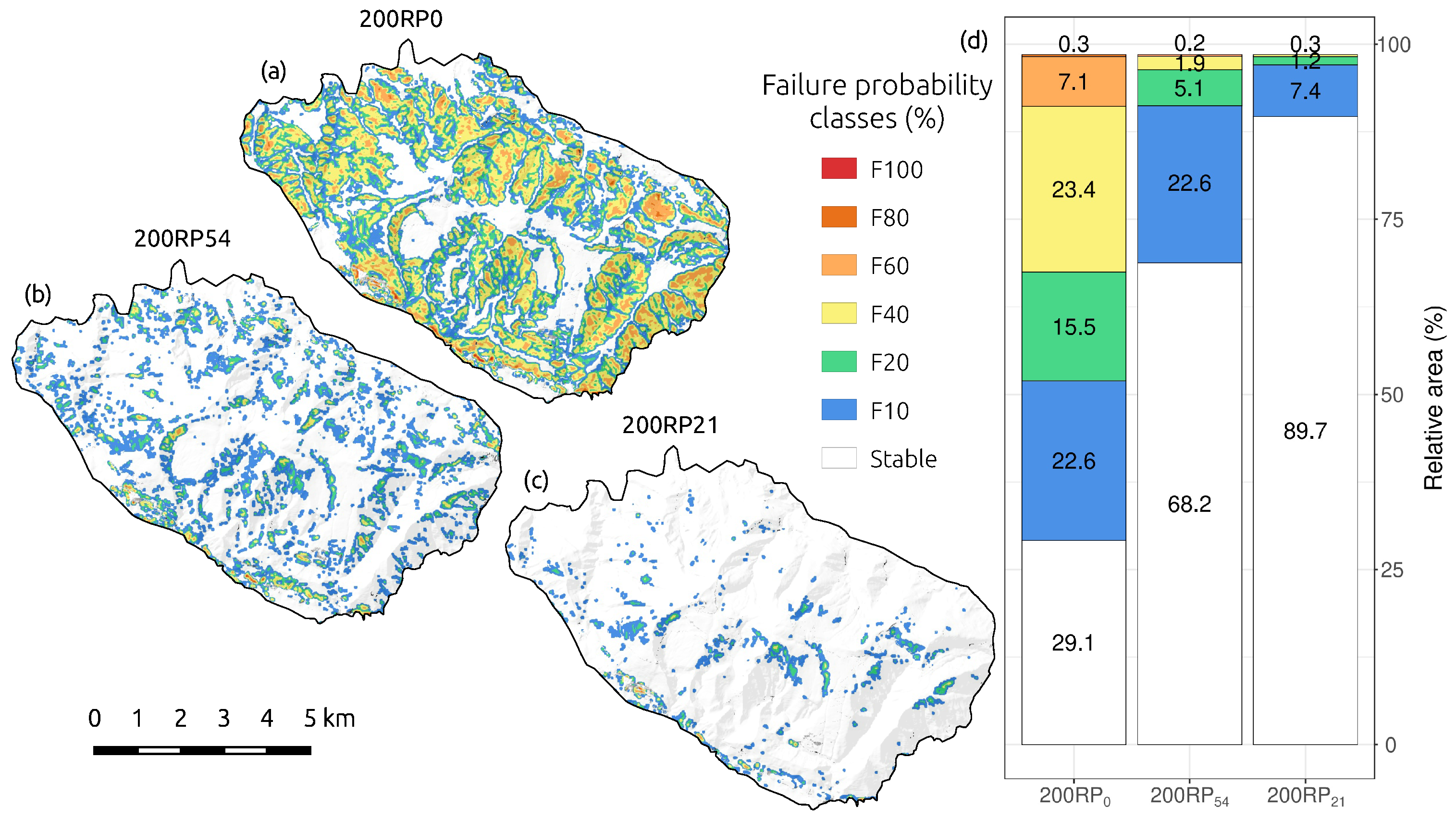
3.2. Effects of Land Cover Changes on Slope Stability (1954–2021)

The effect of land cover changes on slope stability clearly appeared in the three simulation scenarios with a 200-year return period (Figure 4): (a) no-cover (worst scenario, 200 RP 0 ), (b) 1954 land cover ( 200 RP 54 ), and (c) 2021 land cover ( 200 RP 21 ). The no-cover ( 200 RP 0 ) scenario showed that 68.9% of the area, including all failure probability classes (>1% failure probability), is potentially susceptible to landslides. A limited portion of this area is represented by the highest probability classes, namely F60 (7.1%) and F80 (0.3%). The comparison between the 200 RP 0 , 200 RP 54 , and 200 RP 21 scenarios highlighted the effect of vegetation cover. The stable area had doubled in 200 RP 54 compared to 200 RP 0 (68.2% vs. 29.1%) and increased further in 200 RP 21 (89.7%). F10 class areas had remained unchanged in 200 RP 0 and 200 RP 54 (22.6%) but decreased in 200 RP 21 to 7.4%. Significant changes were observed for all three scenarios: the F20 class areas were reduced by one-third in 200 RP 54 compared to 200 RP 0 (15.5% vs. 5.1%) and then decreased again in 200 RP 21 (1.2%); the F40 class areas showed a drastic reduction from 200 RP 54 to 200 RP 21 (23.5% to 1.9%).

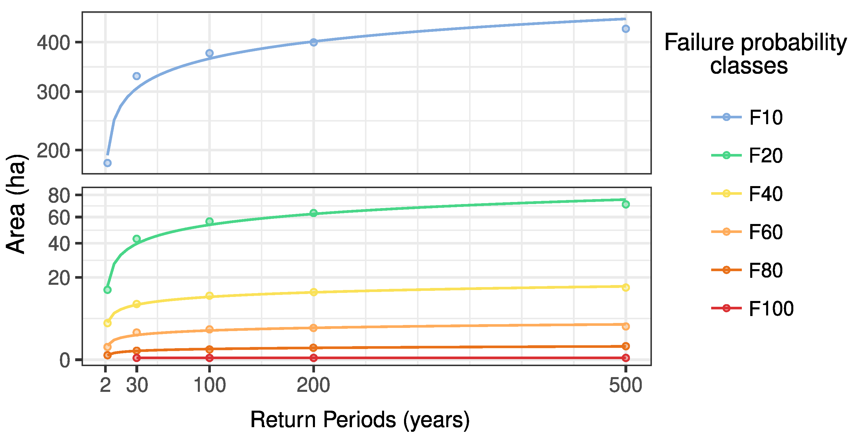
3.3. Slope Stability Assessment with Different Rainfall Return Periods (2021*)

The analysis of slope stability based on the current forested area (forest categories 2021*) and different rainfall return periods showed significant differences in the extension of the area of the failure probability classes (Figure 5). Increasing the return time of rainfall, the total area with a higher risk did not change significantly. On the other hand, the areas with low failure probabilities increased significantly (Figure 5). For example, the F10 areas increased by 200 ha between the 2 and 100-year return period rainfall. The F20 area was 20 to 60 ha for the same RPs. Changes were limited for the remaining failure probability classes (F40, F60) or insignificant (F80 and F100). In particular, the F100 class did not change, even for the 500-year RP variation. In summary, with the current landscape (2021* scenario), low failure probability (F10 and F20) areas showed a significant increase moving from 2RP to 100RP (Figure 5). The greatest change in the area was recorded with a 30-year RP. In general, the greatest increase in unstable areas occurred in the 30RP scenario. The results showed that this rainfall scenario resulted in the presence of areas with significant values of failure probability (F80 and F100), highlighting the predominance of morphological and soil characteristics in the slope stability dynamics of these areas, as well as the ineffectiveness of root reinforcement in these cases.
The low correlation between the variation in the surface area of high failure probability and increasing RPs suggested that geo-morphological and land cover factors drive landslide susceptibility [58,59,60].
The spatial distribution of the failure probability classes in the different forest categories between the no-cover and 2021* scenarios changed significantly (Figure 6). The area distribution for the different return periods remained nearly identical for all forest categories in 2021*. The increase for the F20 and higher classes was very minor. This indicates that forests had an important role in reducing landslide susceptibility for all return periods, whereas the no-vegetation cover scenarios showed a significant surface area increase with high failure probability classes and higher return periods, as we would expect.
Several species occupied areas with high failure probability when running the no-cover scenario. This was particularly true for oak (do) and hornbeam–manna ash (hm) forest cover. These woodlands colonized steeper areas of abandoned pastures that were more prone to landslides. The presence or absence of woodlands significantly affected the spatial distribution of the failure probability, particularly with high values of rainfall return period. For the 2-year RP in holm oak (ho) woodlands, both the no cover and forest cover scenarios showed a nearly 100% area in the F10 failure probability class, indicating that it grows in relatively stable areas. With increasing rainfall rates at higher return periods, the forest-covered areas remained completely stable (nearly a 100% area in F10), while areas with high landslide probability classes increased, indicating the important effect of this species in reducing landslide probability.
The analysis performed using the forest categories confirmed the role of forests in reducing rainfall-induced shallow landslides [61,62,63,64], given the different efficiencies depending on tree species. Such differences derive from their root reinforcement and coefficients (Table 1), considering the forest composition and density. Reduced efficiency is affected by a tree species’ root system type and on-site conditions, slope, and soil depth in particular. Deep root systems, as in Quercus spp. [65], provide the activation of basal root reinforcement, considered the most effective type [26], where roots can reach the deepest and most stable soil layers and provide strong anchoring [66,67]. On the other hand, shallow root systems, like those of most pine species, have a lesser basal root reinforcement that rapidly diminishes with soil depth [59].

3.4. SlideforMAP Validation

We validated the SlideforMAP model for slope failure susceptibility using the 200 RP 54 scenario, through a receiver operating characteristic (ROC) analysis (Figure 7) using the R package called (pROC (https://cran.r-project.org/web/packages/pROC/pROC.pdf, accessed on 9 August 2024). The ROC curve showed an average area under the curve (AUC) of 0.865, with a sensitivity of 0.786 and a specificity of 0.953. An AUC of 0.865 indicated a high level of discriminative ability for the model. With an AUC of 0.865, the model performed well above random chance, effectively distinguishing between the positive and negative classes. This high AUC value signified that the model was robust in identifying true positives and true negatives across different threshold levels. A sensitivity of 0.786 represented a strong performance, with 78.6% of actual positive cases. A specificity, or true negative rate, of 0.953 meant that the model correctly identified approximately 95.3% of the actual negative cases, suggesting that the model was highly effective at ruling out negatives and minimizing false positives.
In summary, the given values suggest that the model was proficient in distinguishing between positive and negative cases, with a strong ability to correctly identify both true positives and true negatives. The high AUC value underscored the model’s excellent discriminative power, while the high sensitivity and specificity balanced each other, indicating a well-optimized model suitable for practical application in scenarios requiring high accuracy and reliability.

4. Conclusions

The spatio-temporal analysis conducted in this work provided an overall understanding of the effects of vegetation cover changes on slope stability. The use of SlideforMAP provided quantitative information about the failure probability, simulating heavy rainfall scenarios and becoming a helpful decision-support tool in land and forest management. We used a series of scenarios encompassing different vegetation covers and rainfall return periods, considered critical conditions in understanding slope stability dynamics in Apennine areas.
The analysis of land use changes over the past 70 years revealed significant ecological transformations, consistent with those of most Italian mountainous areas, with essential implications for landscape diversity and stability. Such shifts modify the ecological balance and influence slope stability, as demonstrated by the simulation scenarios assessing landslide susceptibility under varying rainfall return periods.
Comparing landslide susceptibility in 1954 and 2021 showed how forest cover expansion can decrease landslide probability, especially in areas at higher risk. Abandoned pastures and agricultural crops, shifted to forest, did not determine a significant change in landslide susceptibility, because of their location on gentler slopes. Considering the effect of rainfall intensity with different return times, the extensive vegetation cover in 2021 provides an effective stabilizing effect, at least for rainfall rates with a return period of up to 30 years.
The ongoing land use changes in the Apennines, featuring the loss of agricultural land and the expansion of forest cover, present challenges and opportunities for landscape management. The observed trends suggest the revision of land use policies and the promotion of sustainable practices that enhance biodiversity conservation, while safeguarding against natural hazards such as landslides. Future research should focus on the long-term ecological impacts of these changes and the potential for restoring sustainable practices of traditional land use, fostering overall resilience in these mountainous regions.
Although slope stability models are valuable tools for quantifying the landslide susceptibility of an area, their application in some contexts is still limited. Over the past decade, the development of these models has focused on the protective role of vegetation, considering the complexity of root reinforcement variability [38]. However, the application of these models is still limited in contexts where the details of the available data remain coarse. The presented study is one such case, especially regarding the vegetation component. The lack of detailed land cover data, particularly of a digital elevation and surface model, did not allow using the single-tree analysis option implemented in SlideforMAP and shown in the case study presented by van Zadelhoff et al. [43]. In addition, the lack of a characterization of root reinforcement parameters in forest governance types different from high forest, and in particular the coppice that is typical of the entire Italian Apennines, makes it difficult to use advanced techniques, albeit implemented in the models, and requires the use of assumptions for this factor. Such assumptions introduce a degree of uncertainty into the analysis that must be properly considered when the products obtained from these analyses are used in the planning and design stages.

Author Contributions

Conceptualization, I.M., A.V., F.G. and C.U.; Methodology, I.M., A.V., F.G. and D.C.; Software, M.S.; Investigation, I.M., E.T. and L.B.; Writing—original draft, I.M.; Writing—review & editing, A.V., F.G., E.T., L.B., D.C., M.S. and C.U.; Supervision, A.V., F.G. and C.U.; Funding acquisition, C.U. All authors have read and agreed to the published version of the manuscript.

Funding

This research was funded by PSR Marche 2014/2020 Misura 16.1—Sostegno per la costituzione e la gestione dei gruppi operativi del PEI in materia di produttività e sostenibilità dell’agricoltura Azione 2—Fase di gestione del G.O. e realizzazione del Piano di Attività, grant number BIOSEIFORTE—ID 41339.

Data Availability Statement

No new data were created or analyzed in this study. Data sharing is not applicable to this article.

Conflicts of Interest

Author Denis Cohen was employed by the company CoSci LLC. The remaining authors declare that the research was conducted in the absence of any commercial or financial relationships that could be construed as a potential conflict of interest.

References

  1. Persichillo, M.G.; Bordoni, M.; Meisina, C.; Bartelletti, C.; Barsanti, M.; Giannecchini, R.; D’Amato Avanzi, G.; Galanti, Y.; Cevasco, A.; Brandolini, P.; et al. Shallow landslides susceptibility assessment in different environments. Geomat. Nat. Hazards Risk 2017, 8, 748–771. [Google Scholar] [CrossRef]
  2. Tufano, R.; Formetta, G.; Calcaterra, D.; De Vita, P. Hydrological control of soil thickness spatial variability on the initiation of rainfall-induced shallow landslides using a three-dimensional model. Landslides 2021, 18, 3367–3380. [Google Scholar] [CrossRef]
  3. Montrasio, L.; Valentino, R.; Losi, G.L. Shallow landslides triggered by rainfalls: Modeling of some case histories in the Reggiano Apennine (Emilia Romagna Region, Northern Italy). Nat. Hazards 2012, 60, 1231–1254. [Google Scholar] [CrossRef]
  4. Garbarino, M.; Morresi, D.; Urbinati, C.; Malandra, F.; Motta, R.; Sibona, E.M.; Vitali, A.; Weisberg, P.J. Contrasting land use legacy effects on forest landscape dynamics in the Italian Alps and the Apennines. Landsc. Ecol. 2020, 35, 2679–2694. [Google Scholar] [CrossRef]
  5. Gerrard, J.; Gardner, R. Relationships between landsliding and land use in the Likhu Khola drainage basin, Middle Hills, Nepal. Mt. Res. Dev. 2002, 22, 48–55. [Google Scholar] [CrossRef]
  6. Glade, T. Landslide occurrence as a response to land use change: A review of evidence from New Zealand. Catena 2003, 51, 297–314. [Google Scholar] [CrossRef]
  7. Chen, L.; Guo, Z.; Yin, K.; Shrestha, D.P.; Jin, S. The influence of land use and land cover change on landslide susceptibility: A case study in Zhushan Town, Xuan’en County (Hubei, China). Nat. Hazards Earth Syst. Sci. 2019, 19, 2207–2228. [Google Scholar] [CrossRef]
  8. Malandra, F.; Vitali, A.; Urbinati, C.; Weisberg, P.J.; Garbarino, M. Patterns and drivers of forest landscape change in the Apennines range, Italy. Reg. Environ. Change 2019, 19, 1973–1985. [Google Scholar] [CrossRef]
  9. Branca, G.; Piredda, I.; Scotti, R.; Chessa, L.; Murgia, I.; Ganga, A.; Campus, S.F.; Lovreglio, R.; Guastini, E.; Schwarz, M.; et al. Forest Protection Unifies, Silviculture Divides: A Sociological Analysis of Local Stakeholders’ Voices after Coppicing in the Marganai Forest (Sardinia, Italy). Forests 2020, 11, 708. [Google Scholar] [CrossRef]
  10. Piermattei, A.; Lingua, E.; Urbinati, C.; Garbarino, M. Pinus nigra anthropogenic treelines in the central Apennines show common pattern of tree recruitment. Eur. J. For. Res. 2016, 135, 1119–1130. [Google Scholar] [CrossRef]
  11. Vacchiano, G.; Garbarino, M.; Lingua, E.; Motta, R. Forest dynamics and disturbance regimes in the Italian Apennines. For. Ecol. Manag. 2017, 388, 57–66. [Google Scholar] [CrossRef]
  12. Vitali, A.; Urbinati, C.; Weisberg, P.J.; Urza, A.K.; Garbarino, M. Effects of natural and anthropogenic drivers on land-cover change and treeline dynamics in the Apennines (Italy). J. Veg. Sci. 2018, 29, 189–199. [Google Scholar] [CrossRef]
  13. Flepp, G.; Robyr, R.; Scotti, R.; Giadrossich, F.; Conedera, M.; Vacchiano, G.; Fischer, C.; Ammann, P.; May, D.; Schwarz, M. Temporal Dynamics of Root Reinforcement in European Spruce Forests. Forests 2021, 12, 815. [Google Scholar] [CrossRef]
  14. Gehring, E.; Conedera, M.; Maringer, J.; Giadrossich, F.; Guastini, E.; Schwarz, M. Shallow landslide disposition in burnt European beech (Fagus sylvatica L.) forests. Sci. Rep. 2019, 9, 8638. [Google Scholar] [CrossRef]
  15. Tasser, E.; Mader, M.; Tappeiner, U. Effects of land use in alpine grasslands on the probability of landslides. Basic Appl. Ecol. 2003, 4, 271–280. [Google Scholar] [CrossRef]
  16. Persichillo, M.G.; Bordoni, M.; Meisina, C. The role of land use changes in the distribution of shallow landslides. Sci. Total Environ. 2017, 574, 924–937. [Google Scholar] [CrossRef]
  17. Schmidt, K.; Roering, J.; Stock, J.; Dietrich, W.; Montgomery, D.; Schaub, A.T. The variability of root cohesion as an influence on shallow landslide susceptibility in the Oregon Coast Range. Can. Geotech. J. 2001, 38, 995–1024. [Google Scholar] [CrossRef]
  18. Sidle, R.C.; Ziegler, A.D.; Negishi, J.N.; Nik, A.R.; Siew, R.; Turkelboom, F. Erosion processes in steep terrain—Truths, myths, and uncertainties related to forest management in Southeast Asia. For. Ecol. Manag. 2006, 224, 199–225. [Google Scholar] [CrossRef]
  19. Vacchiano, G.; Berretti, R.; Mondino, E.B.; Meloni, F.; Motta, R. Assessing the effect of disturbances on the functionality of direct protection forests. Mt. Res. Dev. 2016, 36, 41–55. [Google Scholar] [CrossRef]
  20. Kalsnes, B.; Capobianco, V. Use of vegetation for landslide risk mitigation. In Climate Adaptation Modelling; Springer International Publishing: Cham, Switzerland, 2022; pp. 77–85. [Google Scholar]
  21. Phillips, C.; Hales, T.; Smith, H.; Basher, L. Shallow landslides and vegetation at the catchment scale: A perspective. Ecol. Eng. 2021, 173, 106436. [Google Scholar] [CrossRef]
  22. Liu, X.; Lan, H.; Li, L.; Cui, P. An ecological indicator system for shallow landslide analysis. CATENA 2022, 214, 106211. [Google Scholar] [CrossRef]
  23. Mehtab, A.; Jiang, Y.J.; Su, L.J.; Shamsher, S.; Li, J.J.; Mahfuzur, R. Scaling the roots mechanical reinforcement in plantation of Cunninghamia R. Br in Southwest China. Forests 2020, 12, 33. [Google Scholar] [CrossRef]
  24. Schwarz, M.; Lehmann, P.; Or, D. Quantifying lateral root reinforcement in steep slopes—From a bundle of roots to tree stands. Earth Surf. Processes Landforms 2010, 35, 354–367. [Google Scholar] [CrossRef]
  25. Vergani, C.; Giadrossich, F.; Buckley, P.; Conedera, M.; Pividori, M.; Salbitano, F.; Rauch, H.; Lovreglio, R.; Schwarz, M. Root reinforcement dynamics of European coppice woodlands and their effect on shallow landslides: A review. Earth-Sci. Rev. 2017, 167, 88–102. [Google Scholar] [CrossRef]
  26. Cohen, D.; Schwarz, M. Tree-root control of shallow landslides. Earth Surf. Dyn. 2017, 5, 451–477. [Google Scholar] [CrossRef]
  27. Vergani, C.; Graf, F. Soil permeability, aggregate stability and root growth: A pot experiment from a soil bioengineering perspective. Ecohydrology 2016, 9, 830–842. [Google Scholar] [CrossRef]
  28. Schwarz, M.; Rist, A.; Cohen, D.; Giadrossich, F.; Egorov, P.; Büttner, D.; Stolz, M.; Thormann, J.J. Root reinforcement of soils under compression. J. Geophys. Res. Earth Surf. 2015, 120, 2103–2120. [Google Scholar] [CrossRef]
  29. Giadrossich, F.; Cohen, D.; Schwarz, M.; Ganga, A.; Marrosu, R.; Pirastru, M.; Capra, G.F. Large roots dominate the contribution of trees to slope stability. Earth Surf. Processes Landforms 2019, 44, 1602–1609. [Google Scholar] [CrossRef]
  30. Stokes, A.; Atger, C.; Bengough, A.G.; Fourcaud, T.; Sidle, R.C. Desirable plant root traits for protecting natural and engineered slopes against landslides. Plant Soil 2009, 324, 1–30. [Google Scholar] [CrossRef]
  31. Schwarz, M.; Giadrossich, F.; Cohen, D. Modeling root reinforcement using a root-failure Weibull survival function. Hydrol. Earth Syst. Sci. 2013, 17, 4367–4377. [Google Scholar] [CrossRef]
  32. Giadrossich, F.; Schwarz, M.; Cohen, D.; Preti, F.; Or, D. Mechanical interactions between neighbouring roots during pullout tests. Plant Soil 2013, 367, 391–406. [Google Scholar] [CrossRef]
  33. Giadrossich, F.; Schwarz, M.; Marden, M.; Marrosu, R.; Phillips, C. Minimum representative root distribution sampling for calculating slope stability in Pinus radiata D.Don plantations in New Zealand. N. Z. J. For. Sci. 2020, 50. [Google Scholar] [CrossRef]
  34. Ngo, H.M.; Van Zadelhoff, F.B.; Gasparini, I.; Plaschy, J.; Flepp, G.; Dorren, L.; Phillips, C.; Giadrossich, F.; Schwarz, M. Analysis of Poplar’s (Populus nigra ita.) Root Systems for Quantifying Bio-Engineering Measures in New Zealand Pastoral Hill Country. Forests 2023, 14, 1240. [Google Scholar] [CrossRef]
  35. Keim, R.F.; Skaugset, A.E. Modelling effects of forest canopies on slope stability. Hydrol. Processes 2003, 17, 1457–1467. [Google Scholar] [CrossRef]
  36. Cascini, L.; Cuomo, S.; Pastor, M.; Sorbino, G. Modeling of Rainfall-Induced Shallow Landslides of the Flow-Type. J. Geotech. Geoenviron. Eng. 2010, 136, 85–98. [Google Scholar] [CrossRef]
  37. Guillard, C.; Zezere, J. Landslide Susceptibility Assessment and Validation in the Framework of Municipal Planning in Portugal: The Case of Loures Municipality. Environ. Manag. 2012, 50, 721–735. [Google Scholar] [CrossRef]
  38. Murgia, I.; Giadrossich, F.; Mao, Z.; Cohen, D.; Capra, G.F.; Schwarz, M. Modeling shallow landslides and root reinforcement: A review. Ecol. Eng. 2022, 181, 106671. [Google Scholar] [CrossRef]
  39. Mao, Z. Root reinforcement models: Classification, criticism and perspectives. Plant Soil 2022, 472, 17–28. [Google Scholar] [CrossRef]
  40. Cohen, D.; Lehmann, P.; Or, D. Fiber Bundle Model for Multiscale Modeling of Hydromechanical Triggering of Shallow Landslides. Water Resour. Res. 2009, 45, W10436. [Google Scholar] [CrossRef]
  41. Arnone, E.; Caracciolo, D.; Noto, L.V.; Preti, F.; Bras, R.L. Modeling the hydrological and mechanical effect of roots on shallow landslides. Water Resour. Res. 2016, 52, 8590–8612. [Google Scholar] [CrossRef]
  42. Cislaghi, A.; Chiaradia, E.A.; Bischetti, G.B. Including root reinforcement variability in a probabilistic 3D stability model: Root reinforcement variability in a probabilistic 3-D stability model. Earth Surf. Processes Landforms 2017, 42, 1789–1806. [Google Scholar] [CrossRef]
  43. Van Zadelhoff, F.B.; Albaba, A.; Cohen, D.; Phillips, C.; Schaefli, B.; Dorren, L.; Schwarz, M. Introducing SlideforMAP: A probabilistic finite slope approach for modelling shallow-landslide probability in forested situations. Nat. Hazards Earth Syst. Sci. 2022, 22, 2611–2635. [Google Scholar] [CrossRef]
  44. Cornes, R.C.; van der Schrier, G.; van den Besselaar, E.J.; Jones, P.D. An ensemble version of the E-OBS temperature and precipitation data sets. J. Geophys. Res. Atmos. 2018, 123, 9391–9409. [Google Scholar] [CrossRef]
  45. Rivas-Martínez, S.; Rivas-Saenz, S.; Penas, A. Worldwide Bioclimatic Classification System; Backhuys Pub.: Kerkwerve, The Netherlands, 2002. [Google Scholar]
  46. De Donatis, M.; Alberti, M.; Cipicchia, M.; Guerrero, N.M.; Pappafico, G.F.; Susini, S. Workflow of Digital Field Mapping and Drone-Aided Survey for the Identification and Characterization of Capable Faults: The Case of a Normal Fault System in the Monte Nerone Area (Northern Apennines, Italy). ISPRS Int. J.-Geo-Inf. 2020, 9, 616. [Google Scholar] [CrossRef]
  47. Tamburini, A. Structural characterization of a carbonate hydrostructures in the Umbria-Marche Apennines. Rend. Online Della Soc. Geol. Ital. 2016, 41, 88–91. [Google Scholar] [CrossRef]
  48. Tarquini, S.; Isola, I.; Favalli, M.; Battistini, A.; Dotta, G.T. A Digital Elevation Model of Italy with a 10 Meters Cell Size (Version 1.1); Istituto Nazionale di Geofisica e Vulcanologia (INGV): Roma, Italy, 2023; Volume 1, pp. 1–2. [Google Scholar] [CrossRef]
  49. Garbarino, M.; Lingua, E.; Weisberg, P.J.; Bottero, A.; Meloni, F.; Motta, R. Land-use history and topographic gradients as driving factors of subalpine Larix decidua forests. Landsc. Ecol. 2013, 28, 805–817. [Google Scholar] [CrossRef]
  50. Vanacker, V.; Vanderschaeghe, M.; Govers, G.; Willems, E.; Poesen, J.; Deckers, J.; De Bievre, B. Linking hydrological, infinite slope stability and land-use change models through GIS for assessing the impact of deforestation on slope stability in high Andean watersheds. Geomorphology 2003, 52, 299–315. [Google Scholar] [CrossRef]
  51. Shu, H.; Hürlimann, M.; Molowny-Horas, R.; González, M.; Pinyol, J.; Abancó, C.; Ma, J. Relation between land cover and landslide susceptibility in Val d’Aran, Pyrenees (Spain): Historical aspects, present situation and forward prediction. Sci. Total Environ. 2019, 693, 133557. [Google Scholar] [CrossRef]
  52. Jung, M. LecoS—A python plugin for automated landscape ecology analysis. Ecol. Inform. 2016, 31, 18–21. [Google Scholar] [CrossRef]
  53. IPLA. I Tipi Forestali Delle MARCHE: Inventario e Carta Forestale Della Regione Marche; Regione Marche: Marche, Italy, 2001. [Google Scholar]
  54. Molducci, P.; Mazzetto, T.; Casamenti, L. Piano Particolareggiato di Assestamento Forestale’ Consorzio Forestale Monte Nerone; Relazione Tecnica Generale’ Regione Marche: Marche, Italy, 2020. [Google Scholar]
  55. Piano Assetto Idrogeologico. Norme di Attuazione; Technical Report; Regione Marche Autorità di Bacino: Marche, Italy, 2003. [Google Scholar]
  56. ISPRA. Landslide in Italy; Special Report; ISPRA: Varese, Italy, 2008. [Google Scholar]
  57. Pallotta, E.; Boccia, L.; Rossi, C.M.; Ripa, M.N. Forest dynamic in the Italian Apennines. Appl. Sci. 2022, 12, 2474. [Google Scholar] [CrossRef]
  58. Borgatti, L.; Soldati, M. Landslides as a geomorphological proxy for climate change: A record from the Dolomites (northern Italy). Geomorphology 2010, 120, 56–64. [Google Scholar] [CrossRef]
  59. Scheidl, C.; Heiser, M.; Kamper, S.; Thaler, T.; Klebinder, K.; Nagl, F.; Lechner, V.; Markart, G.; Rammer, W.; Seidl, R. The influence of climate change and canopy disturbances on landslide susceptibility in headwater catchments. Sci. Total Environ. 2020, 742, 140588. [Google Scholar] [CrossRef]
  60. Hürlimann, M.; Guo, Z.; Puig-Polo, C.; Medina, V. Impacts of future climate and land cover changes on landslide susceptibility: Regional scale modelling in the Val d’Aran region (Pyrenees, Spain). Landslides 2022, 19, 99–118. [Google Scholar] [CrossRef]
  61. Preti, F. Forest protection and protection forest: Tree root degradation over hydrological shallow landslides triggering. Ecol. Eng. 2013, 61, 633–645. [Google Scholar] [CrossRef]
  62. Moos, C.; Bebi, P.; Graf, F.; Mattli, J.; Rickli, C.; Schwarz, M. How does forest structure affect root reinforcement and susceptibility to shallow landslides? A Case Study in St Antönien, Switzerland. Earth Surf. Processes Landforms 2016, 41, 951–960. [Google Scholar] [CrossRef]
  63. Jurchescu, M.; Kucsicsa, G.; Micu, M.; Bălteanu, D.; Sima, M.; Popovici, E.A. Implications of future land-use/cover pattern change on landslide susceptibility at a national level: A scenario-based analysis in Romania. CATENA 2023, 231, 107330. [Google Scholar] [CrossRef]
  64. Bezak, N.; Jemec Auflič, M.; Mikoš, M. Application of hydrological modelling for temporal prediction of rainfall-induced shallow landslides. Landslides 2019, 16, 1273–1283. [Google Scholar] [CrossRef]
  65. Ghestem, M.; Sidle, R.C.; Stokes, A. The Influence of Plant Root Systems on Subsurface Flow: Implications for Slope Stability. BioScience 2011, 61, 869–879. [Google Scholar] [CrossRef]
  66. Bischetti, G.B.; Chiaradia, E.A.; Epis, T.; Morlotti, E. Root cohesion of forest species in the Italian Alps. Plant Soil 2009, 324, 71–89. [Google Scholar] [CrossRef]
  67. Guns, M.; Vanacker, V. Forest cover change trajectories and their impact on landslide occurrence in the tropical Andes. Environ. Earth Sci. 2013, 70, 2941–2952. [Google Scholar] [CrossRef]
Figure 1. Location of the Mt. Nerone study area (yellow boundaries) in the Central Apennines (red dot).
Land 13 01575 g001
Figure 2. Workflow diagram. Boxes with dashed edges relate to the preliminary step for determining land cover changes. The flowchart elements are color-coded and shaped differently to highlight various workflow stages. Boxes with solid edges indicate the process of slope stability analysis. Data sources (gray cylinder), source data for stability assessment (light blue boxes), software (yellow box shapes), and outputs (dark blue boxes) for the different scenarios (0 = no vegetation cover; 54 = vegetation cover in 1954; 21 = vegetation cover in 2021; 21* = vegetation cover 2021 with detailed forest categories). The bulleted list to the right lists the analyses and comparisons carried out in this research.
Land 13 01575 g002
Figure 3. Land cover in the Mt. Nerone area in 1954 (a) and 2021 (b).
Land 13 01575 g003
Figure 4. Failure probabilities estimated using SlideforMAP for the 200-year return period rainfall with (a) no vegetation cover, (b) 1954 land cover, and (c) 2021 land cover. In the legend, Fn represents the failure probability class, where n is the maximum value of each class. In (d), the sum of the relative areas is less than 100% because urban areas (ua) and roads and paths (rt) were not included.
Land 13 01575 g004
Figure 5. Surface areas with different failure probability classes and different return periods in the 2021* scenario.
Land 13 01575 g005
Figure 6. Area extent (in hectares) of each failure probability class, referring to each forest category (rows) and return period (columns) and comparing no-cover (red bars) and 2021* (blue bars) scenarios. Holm oak (ho), downy oak (do), hop hornbeam–manna ash (hm), beech (be), and turkey oak (to), black pine (bp).
Land 13 01575 g006
Figure 7. ROC curves for predictive model performance at various random point distances. The curves show the area under the curve (AUC) for random point minimum distances of 1, 5, 10, 15, and 20 m. The diagonal dotted line is the reference line that defines the ROC curve as a random classification.
Land 13 01575 g007
Table 1. The 12 scenarios considered, reporting for each return period (RP), relative rainfall intensity, and land cover scenarios. Subscript 0 = no vegetation, 54 = vegetation in 1954, and 21 = vegetation in 2021. The land cover 2021, which considers the forest categories, uses the symbol 21*.
LabelscenarioLand CoverReturn PeriodRainfall (mm)
2 RP 0 no vegetation227
2 RP 21 *2021
30 RP 0 no vegetation3051
30 RP 21 *2021
100 RP 0 no vegetation10061
100 RP 21 *2021
200 RP 0 no vegetation20066
200 RP 54 1954
200 RP 21 2021
200 RP 21 *2021
500 RP 0 no vegetation50074
500 RP 21 *2021
Table 2. Values of root reinforcement (RR), shape, and scale coefficient assigned to each land cover class or forest category (Holm oak—Quercus ilex L.; Downy oak—Quercus pubescens L.; Hop hornbeam—Ostrya carpinifolia Scop.; Manna ash—Fraxinus ornus; Beech—Fagus sylvatica L., Turkey oak—Quercus cerris L.). Detailed values assigned to forest categories are considered only in 21* scenarios. a Vanacker et al. [50], b Shu et al. [51], c estimated by SlideforNET (https://www.ecorisq.org/slidefor-net-en, accessed on 15 March 2023).
Land Cover ClassForest CategoryLabelRR (kPa)ShapeScale
Croplands cr0 a00
Tree groves tg310.1
Unveg. areas un0 a00
Pastures ps0.5 b0.50.1
Other woodlands wl310.1
Broadleaf for. bf10 c2.070.1
Holm oak for.ho10 c2.670.17
Downy oak for.do10 c2.670.17
Hornbeam/Ash for.hm10 c2.070.1
Beech for.be10 c1.280.27
Turkey oak for.to10 c2.670.17
Coniferous for. cf5 c1.140.15
Black pine plant.bp5 c1.140.15
Table 3. Land cover changes expressed as absolute values (hectares) and relative share or landscape values (%) of each class.
LabelLand CoverAbsolute ClassRelative ClassRelative Landscape
IdClassesChange (ha)Change (%)Change (%)
crCroplands−508.3−80%−9.09%
tgTree groves−66.3−73%−1.18%
unUnveg. areas−322.8−94%−5.77%
psPastures−271.0−22%−4.84%
wlOther woodlands−516.5−78%−9.23%
bfBroadleaf for.1634.364%29.21%
cfConiferous for.25.7224%0.46%
rtroads and paths−2.0−5%−0.04%
uaurban areas26.8122%0.48%
Disclaimer/Publisher’s Note: The statements, opinions and data contained in all publications are solely those of the individual author(s) and contributor(s) and not of MDPI and/or the editor(s). MDPI and/or the editor(s) disclaim responsibility for any injury to people or property resulting from any ideas, methods, instructions or products referred to in the content.

