SkipResNet: Crop and Weed Recognition Based on the Improved ResNet

Abstract

Weeds have a detrimental effect on crop yield. However, the prevailing chemical weed control methods cause pollution of the ecosystem and land. Therefore, it has become a trend to reduce dependence on herbicides; realize a sustainable, intelligent weed control method; and protect the land. In order to realize intelligent weeding, efficient and accurate crop and weed recognition is necessary. Convolutional neural networks (CNNs) are widely applied for weed and crop recognition due to their high speed and efficiency. In this paper, a multi-path input skip-residual network (SkipResNet) was put forward to upgrade the classification function of weeds and crops. It improved the residual block in the ResNet model and combined three different path selection algorithms. Experiments showed that on the plant seedling dataset, our proposed network achieved an accuracy of 95.07%, which is 0.73%, 0.37%, and 4.75% better than that of ResNet18, VGG19, and MobileNetV2, respectively. The validation results on the weed–corn dataset also showed that the algorithm can provide more accurate identification of weeds and crops, thereby reducing land contamination during the weeding process. In addition, the algorithm is generalizable and can be used in image classification in agriculture and other fields.

1. Introduction

With the support of relevant national policies for modern agriculture, China, as a major agricultural country, has considerably improved its level of agricultural intelligence [1]. Deep learning techniques, after continuous development, have been applied in various image classification fields, including agriculture [2]. Agricultural image recognition technology combines the advantages of automated processing, analysis of agricultural data, and remote control of automation control technology, which not only avoids the problems of traditional methods that require human intervention and ensures a certain degree of accuracy but also saves labor costs, provides reasonable suggestions for agricultural work, and, thus, realizes efficient agricultural intelligence [3].

Weeds in the field often grow faster than crops and compete for crop growth resources. In addition, they attract pests and diseases to spread viruses [4]. If left untreated, this can lead to lower crop yields. For example, in the case of corn, the yield is positively correlated with the effectiveness of weed control. Controlling weeds within the first 6–8 weeks after sowing is crucial. For effective control, weeds first need to be properly identified. Chemical herbicides are still our first choice for weed control, and spraying herbicides evenly is the most common method of weed control. This method not only affects crop yields but also contaminates soil and water sources, which in turn affects the entire farm ecosystem. In order to effectively protect the environment and ensure a high crop yield, intelligent weeding has become an important research direction. As a result, various types of weeding robots have emerged, such as composite intelligent in-row weeding robots [5] and all-weather laser intelligent weeding robots. Intelligent weeding involves spraying herbicides in a specific area, the most critical issue being the automatic recognition of agricultural crops and grass weeds with high precision. Therefore, accurate categorization of crops and weeds is important for agricultural management and food security [6].

Feature-based approaches

In early research on machine-learning-based weed recognition, image features, such as the color [7], texture [8], shape [9], and edges [10], of weeds were widely used. Bakhshipour et al. [11] extracted 52 textural features of weeds using principal component analysis and selected 14 features from them for inter-crop weed classification. Le and his partners [12] thought hard about an approach combining a support vector machine (SVM) together with a binary pattern operator to extract leaf texture features and validated it in four categories of plant classification. In [8], Sabzi and his partners conceptualized a classification system to recognize potatoes and weeds that uses the color and texture features of plants and can be tested with 98% accuracy. Yanxia Sun et al. [13] considered green pixels outside the target of green vegetable seedlings as weeds, segmented weeds using color features, and investigated the effect of mainstream CNNs and emerging transformer neural networks on green vegetable recognition.

However, there are many types of weeds with different characteristics. It is difficult to extract features that have a universal effect. Meanwhile, texture, color, etc., are all based on manual design, which can be blind [14].

CNN-based approaches

The emergence of CNNs brings a new direction in weed recognition. Convolutional neural networks have been validated by researchers to be more efficient than classical machine learning algorithms [15]. A CNN can acquire global features and contextual information of sample images in pictures and complete images [16]. A CNN automatically learns features from image samples during its own training process and then extracts higher-dimensional, abstract features. The extracted features have a higher correlation with the classifiers, which effectively solves the problems of manually extracting features and classifier selection [17].

In 2016, Dyrmann et al. [18] proposed the use of CNNs to classify color plant images and combined six different plant datasets containing 22 classes of weeds and crops at various growth stages. The results of many tests showed that it was the most advanced weed recognition method at that time. Later, the CNN was widely used in research on weed recognition. In [19], the authors used CNNs for weed detection in soybean crops, with the aim of applying specific herbicides to weeds to avoid affecting soybean yields. Zhang et al. [20] used the Faster R-CNN deep network model to share convolutional features. The results in oilseed rape and weed recognition showed that the Faster R-CNN deep network model based on VGG-16 could recognize oilseed rape and weeds with a precision of up to 83.90%, a recall rate of 78.86%, and an F1 value of 81.30%. In [21], a classification method for corn, narrow-leaf weeds, and broad-leaf weeds was proposed using a CNN, with an accuracy of 97%. Luo et al. [22] carried out the recognition of 140 weeds on six network architectures: AlexNet, GoogLeNet, VGG16, SqueezeNet, Xception, and NasNet-Mobile. Babu et al. [23] added contrast finite adaptive histogram equalization to the residual CNN to classify soils, grasses, soybeans, and broad leaves, which achieved an accuracy of 97.3%. Tao et al. [16] used an SVM classifier in a CNN to classify winter oilseed rape and the weeds around it and achieved a classification accuracy of 92.1%. Manikandakumar et al. [24] incorporated a particle swarm optimization technique in a CNN to classify weeds. The classification accuracy of the CNN reached 98.58% on the TNAU dataset and 97.79% on the ICAR-DWR dataset. In order to overcome the limitation of unimodal information on grass weeds, Xu et al. [25] constructed a dual-path feature extraction network, WeedsNet, which fuses multimodal information by using appropriate CNNs to extract weed features from both RGB and depth images. The accuracy of weed detection in natural wheat fields was 62.3%. The method can work well for weeds and crops with extremely similar visual characteristics. All of these studies have investigated crop and weed classification by deep learning, which achieved better experimental results than traditional methods and strongly promoted the development of intelligent weeding.

However, nowadays, most of the neural network models based on deep learning ignore the information generated by the intermediate layer, wasting an extensive amount of data generated by the image in the process of training in passing through models. The first problem is the insufficient use of information. The original feature information gradually disappears when the data are propagated through multiple layers. The emergence of ResNet [26] has solved the problem of gradient disappearance [27] during network deepening. ResNet can keep more features by “residual connection”, but the network layers near the output still cannot effectively obtain the original features. In addition, the deep CNN architecture lacks flexibility. Therefore, we had an idea for a weed image recognition system based on a multi-path input skip-residual neural network in view of the residual network to enhance the accuracy of weed recognition. It will provide new research ideas for efficient and accurate automated weed control and promote the intelligent development of agriculture.

In this paper, we mainly carried out the following:

• This paper constructed three different path selection algorithms for multi-path input skip-residual neural networks, which were the minimum loss value path selection algorithm, the individual optimal path selection algorithm, and the optimal path statistical selection algorithm.
• This paper proposed a multi-path input skip-residual neural network on the basis of the residual network and combined the three path selection algorithms to be verified on the plant seedling dataset and the weed–corn dataset for the efficient classification of crops and weeds.
• The proposed multi-path input and path selection algorithms were validated on the CIFAR-10 dataset, illustrating the feasibility of the method for other image classification.

2. Materials and Methods

In this section, the focus was on the network models and algorithms, evaluation metrics, datasets, and data processing methods used to perform the image classification task. As shown in Figure 1, the whole classification task consisted of five main steps. First, the dataset (open source datasets used in this thesis) is constructed, and the data are processed and enhanced. Next, features are extracted through the convolutional layer of various network models, and then, image classification is performed.

2.1. Network Models and Algorithms

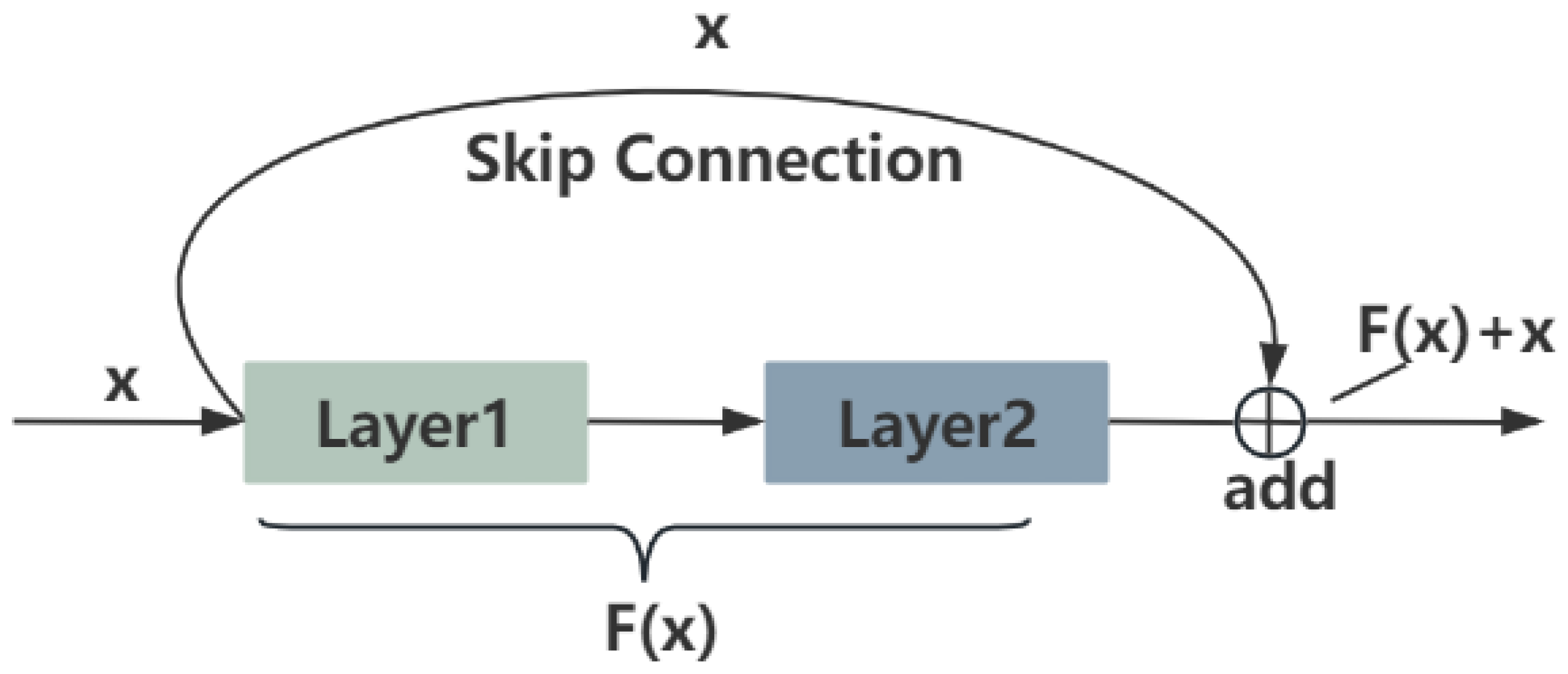
2.1.1. ResNet

ResNet is a deep CNN structure proposed by four researchers, including Kaiming He, in 2015 [26]. Before ResNet, the development of the deep CNN encountered a bottleneck. Researchers tried to deepen network layers to increase accuracy. However, it did not work out as well as they had hoped. This is known as the deep network degradation problem. The emergence of ResNet solved this problem. In ResNet, the concept of “residual blocks” was introduced, as shown in Figure 2, allowing the network to transfer information across multiple layers without causing the gradient to disappear. In ResNet, each residual block contains a skip connection. It allows information to be passed directly across multiple layers, allowing the network to learn features at a deeper level.

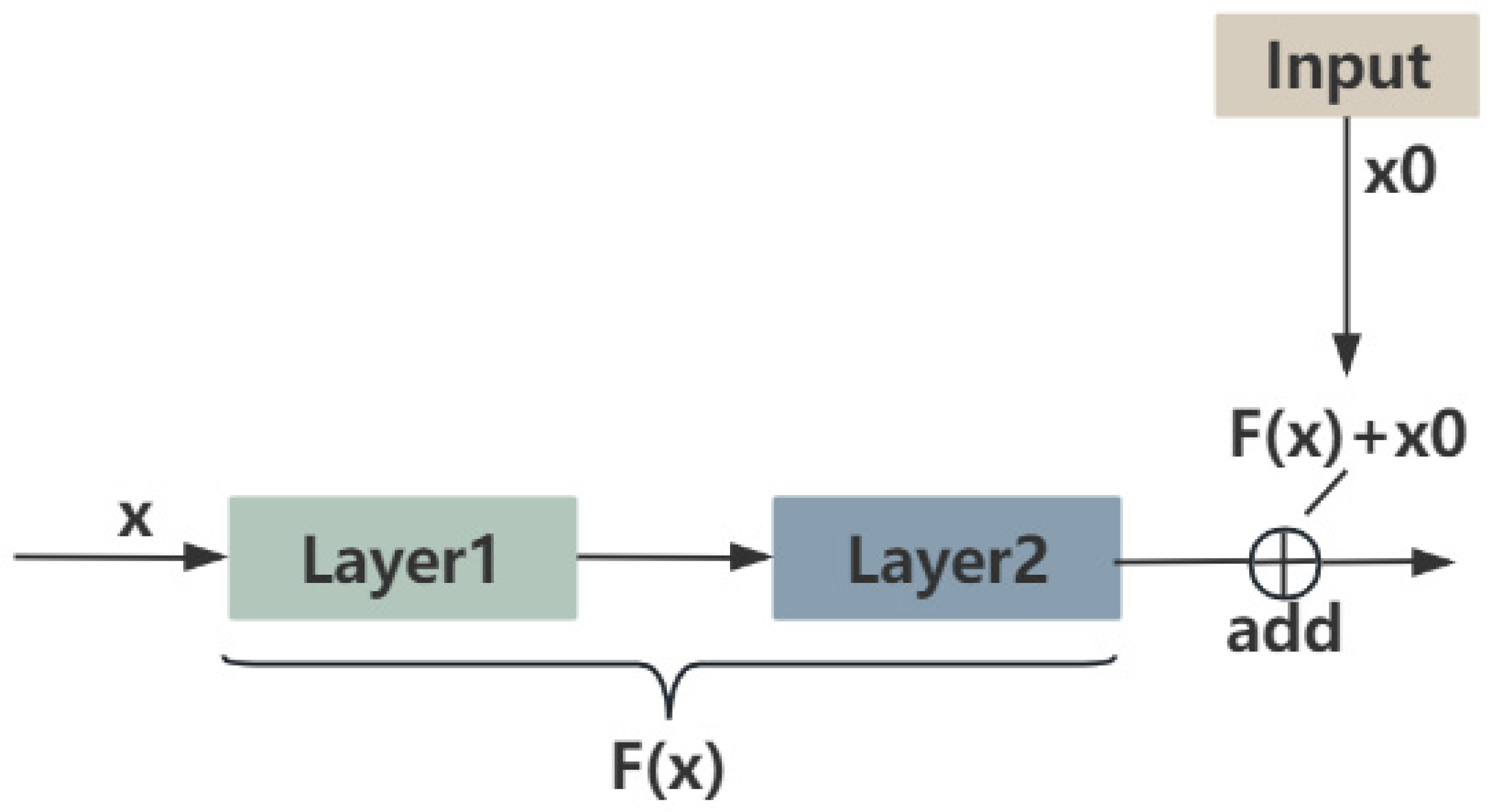
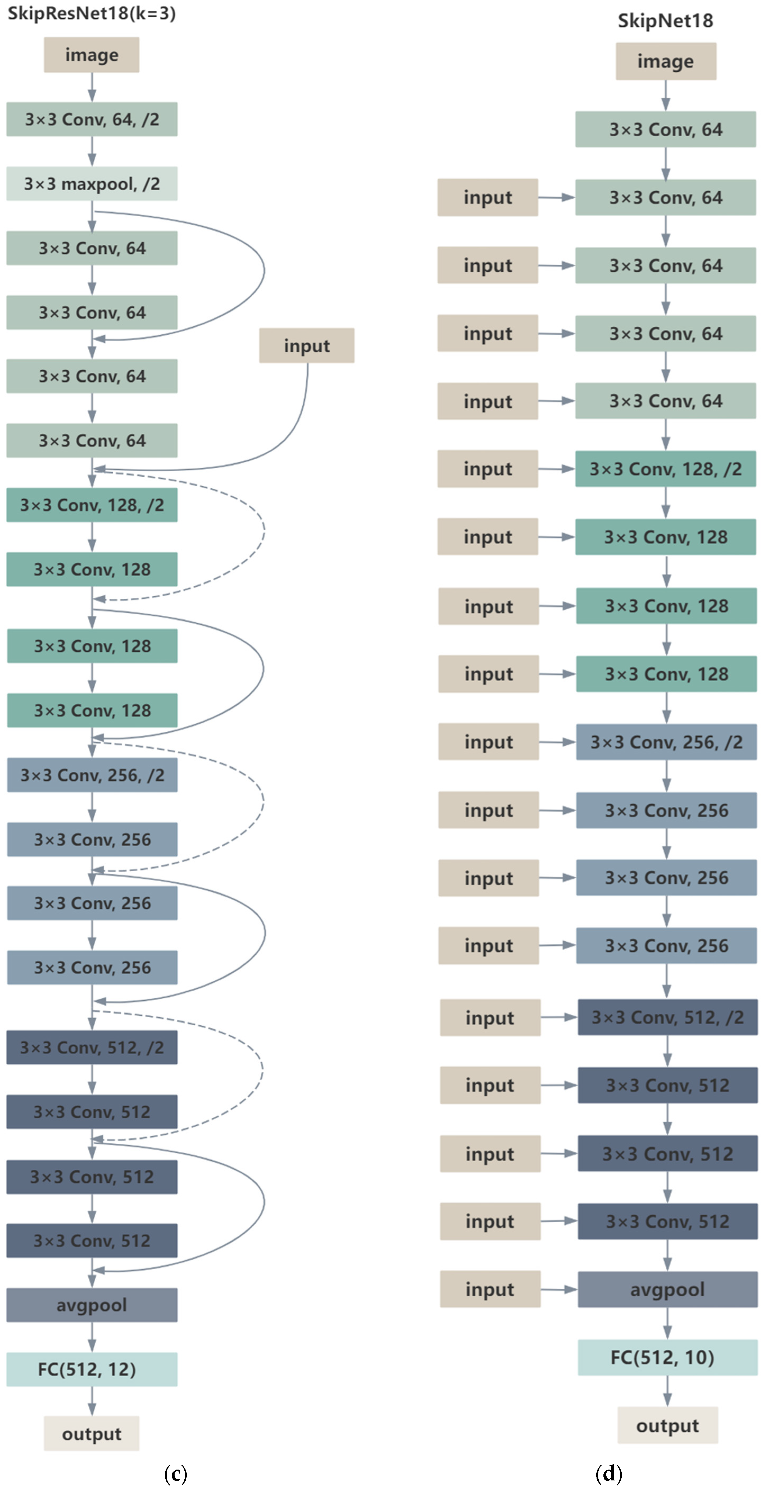
2.1.2. SkipResNet and SkipNet

SkipResNet: This paper mimicked the main structure of the 18-layer ResNet model to propose a multi-path skip-residual neural network (referred to as SkipResNet) in conjunction with the multi-path selection algorithm proposed later. The residual block in ResNet contains a skip connection. The data from the antecedent layer are summed with the output data from that layer and fed into the next layer to continue feature learning. As can be seen from Figure 2, the input data for the next layer eventually become x + F(x). We modified this skip connection to be the result of adding the original input data and data out of the layer to become data in the next layer. As shown in Figure 3, eventually, the input data for the next layer become x0 + F(x). One input path is set in each residual block, there are 9 input paths in SkipResNet18, and the three path selection algorithms proposed later are used to jointly update the network parameters for training.

The structure of SkipResNet18 is shown in Figure 4a–c, with a total of eight initial data input paths in the middle layer and a 1 × 1 convolutional kernel for feature dimension matching. In

Table 1. Details of each network level when SkipResNet18 was trained on the plant seedling dataset.

Layer	Data Out Size	SkipResNet18
conv1	64 × 64	3 × 3, 64, s = 2
conv2	32 × 32	3 × 3 max pool, s = 2
		$\left[\begin{array}{cc}3\times 3,& 64\\ 3\times 3,& 64\end{array}\right]$ × 2
conv3	16 × 16	$\left[\begin{array}{cc}3\times 3,& 128\\ 3\times 3,& 128\end{array}\right]$ × 2
conv4	8 × 8	$\left[\begin{array}{cc}3\times 3,& 256\\ 3\times 3,& 256\end{array}\right]$ × 2
conv5	4 × 4	$\left[\begin{array}{cc}3\times 3,& 512\\ 3\times 3,& 512\end{array}\right]$ × 2
	1 × 1	average pool, 12-d fc, softmax

, the details of each network level when SkipResNet18 acted on the plant seedling dataset are shown.

SkipNet: To validate the multi-path input module and the path selection algorithm proposed in this paper, we removed the residual block of ResNet18, retained the framework of other layers, and set the initial data input path in the middle layer. The new 18-layer network designed is called a multi-path input skipping neural network (referred to as SkipNet18). The network is set up with a total of 18 input paths, and each path is computed individually when each batch of images is fed into the model, without the paths affecting each other. When this batch is back-propagated, the network parameters are jointly updated using the three path selection algorithms we have designed. Our proposed network was evaluated using CIFAR-10, a classical dataset in image classification. The framework of SkipNet18 is displayed in Figure 4d.

2.1.3. Path Selection Algorithm

For the purpose of better leveraging the capability of our network architecture, we designed three path selection algorithms. These path selection algorithms were used while training the new network to act on the input data in the network for path selection and gradient back-propagation.

The minimum loss value path selection algorithm: During the network training process, we package multiple image data into a batch. The whole batch enters the network from different input paths and is finally output at the last layer. The cross-entropy between the output value obtained from each path and the label is calculated. Next, the output path with the smallest loss value of all paths is selected for this batch. This is shown in Equation (1).

$${\mathrm{l}\mathrm{o}\mathrm{s}\mathrm{s}}_{\mathrm{k}}\left(\mathrm{y},\widehat{\mathrm{y}}\right)={\mathrm{m}\mathrm{i}\mathrm{n}}_{\mathrm{k}}(-{\sum }_{\mathrm{i}=1}^{\mathrm{n}}{\mathrm{y}}_{\mathrm{i}}\mathrm{l}\mathrm{o}\mathrm{g}\widehat{{\mathrm{y}}_{\mathrm{i}}}),$$

(1)

The individual optimal path selection algorithm: During the process of network training, for each picture input into a batch in the network, each path can output the predictive values of different classifications of this picture. We choose the path with the greatest predictive value as the optimal path for this picture, then combine the predictive values of each picture in the whole batch, and calculate cross-entropy with the label as a whole to obtain the final loss value of the whole batch. It is equivalent to selecting the optimal path for each image in a batch. Equation (2) is as follows:

$${\mathrm{l}\mathrm{o}\mathrm{s}\mathrm{s}}^{\prime }\left(\mathrm{y},\widehat{\mathrm{y}}\right)={\sum }_{\mathrm{i}=1}^{\mathrm{m}}{\mathrm{m}\mathrm{i}\mathrm{n}}_{{\mathrm{L}}_{\mathrm{i}}}\{-{\sum }_{\mathrm{i}=1}^{\mathrm{n}}{\mathrm{x}}_{\mathrm{i}}\mathrm{l}\mathrm{o}\mathrm{g}\widehat{{\mathrm{x}}_{\mathrm{i}}}\},$$

(2)

The optimal path statistics selection algorithm: During the process of network training, for each image in a batch, the input network can obtain predicted values under different paths, and the path with the largest predicted value is chosen as the most suitable path for this image. At this point, each image is calculated to obtain its corresponding optimal path, and then the path with the highest number of optimal paths selected for different images in a batch is counted as the path selected for the entire batch. Under the selected input path, the pictures of the whole batch enter the network to obtain the output value, and then, cross-entropy with the label is calculated to obtain the loss value of the whole batch. This is shown in Equation (3).

$${\mathrm{l}\mathrm{o}\mathrm{s}\mathrm{s}}_{\mathrm{L}}\left(\mathrm{y},\widehat{\mathrm{y}}\right)=-{\sum }_{\mathrm{i}=1}^{\mathrm{n}}{\mathrm{y}}_{\mathrm{i}}\mathrm{l}\mathrm{o}\mathrm{g}\widehat{{\mathrm{y}}_{\mathrm{i}}},$$

(3)

In Equations (1)–(3), n is the total number of categories, m is the number of images in a batch, ${\mathrm{y}}_{\mathrm{i}}$ and ${\mathrm{x}}_{\mathrm{i}}$ denote the probability that the sample belongs to category i, and $\widehat{{\mathrm{y}}_{\mathrm{i}}}$ and $\widehat{{\mathrm{x}}_{\mathrm{i}}}$ denote the probability that the predicted sample belongs to category i.

The aforementioned three path selection algorithms work together on a batch input into the network to obtain the overall loss value, as shown in Equation (4). Here, $\mathrm{l}\mathrm{o}\mathrm{s}{\mathrm{s}}_{\mathrm{K}}\left(\mathrm{X}\right)$ is the loss value of the whole batch, calculated by selecting path K under the minimum loss value path selection algorithm; $\mathrm{l}\mathrm{o}\mathrm{s}{\mathrm{s}}^{\prime }\left(\mathrm{X}\right)$ represents the loss value of the whole batch calculated under the individual optimal path selection algorithm; $\mathrm{l}\mathrm{o}\mathrm{s}{\mathrm{s}}_{\mathrm{L}}\left(\mathrm{X}\right)$ represents the loss value of the whole batch calculated by selecting path L under the optimal path statistics selection algorithm; and $\mathrm{l}\mathrm{o}\mathrm{s}\mathrm{s}\left(\mathrm{X}\right)$ represents the loss value of the whole batch that enters the multi-path input skipping neural network in this round.

$$\begin{array}{c}\mathrm{L}\mathrm{o}\mathrm{s}\mathrm{s}\left(\mathrm{X}\right)=\mathrm{l}\mathrm{o}\mathrm{s}{\mathrm{s}}_{\mathrm{K}}\left(\mathrm{X}\right)+\mathrm{l}\mathrm{o}\mathrm{s}{\mathrm{s}}^{\prime }\left(\mathrm{X}\right)+\mathrm{l}\mathrm{o}\mathrm{s}{\mathrm{s}}_{\mathrm{L}}\left(\mathrm{X}\right)\end{array},$$

(4)

When conducting network training, we back-propagate the loss value $\mathrm{L}\mathrm{o}\mathrm{s}\mathrm{s}\left(\mathrm{X}\right)$ obtained by each batch under the action of three path selection algorithms, then update the parameters, train the next batch in turn, and so on, until the model performance converges.

To speed up the calculation and processing of image information by the network, this paper chose the third path selection algorithm as the basis for selecting the path of an image sample batch during the test.

2.2. Evaluating Indicator

Here, we introduce some evaluation indicators used in this experiment.

The confusion matrix [28] shows the correspondence between the classification results of the network on the test set and those on the real tags. The tags predicted include true positive (TP), false positive (FP), true negative (TN), and false negative (FN).

Accuracy refers to the ratio of the correctly classified samples in the test set to the total samples. It is one of the important metrics to evaluate the capability of a classification model. In binary classification problems, Equation (5) provides a good representation.

$$\begin{array}{c}\mathrm{A}\mathrm{c}\mathrm{c}\mathrm{u}\mathrm{r}\mathrm{a}\mathrm{c}\mathrm{y}={\displaystyle \frac{\mathrm{T}\mathrm{P}+\mathrm{T}\mathrm{N}}{\mathrm{T}\mathrm{P}+\mathrm{F}\mathrm{P}+\mathrm{F}\mathrm{N}+\mathrm{T}\mathrm{N}}}\end{array},$$

(5)

In multi-classification problems, the accuracy calculation method is similar to that in binary classification problems. For example, in the CIFAR-10 dataset, there are a total of 10 categories, so accuracy can be calculated using Equation (6).

$$\mathrm{A}\mathrm{c}\mathrm{c}\mathrm{u}\mathrm{r}\mathrm{a}\mathrm{c}\mathrm{y}={\displaystyle \frac{{\sum }_{\mathrm{i}=1}^{10}\mathrm{T}{\mathrm{P}}_{\mathrm{i}}}{{\sum }_{\mathrm{i}=1}^{10}(\mathrm{T}{\mathrm{P}}_{\mathrm{i}}+\mathrm{F}{\mathrm{P}}_{\mathrm{i}})}},$$

(6)

The recall rate (or sensitivity) can be measured as the capacity of a classification model to recognize positive examples of samples. This means that the proportion of samples correctly forecasted by the classifier is a positive example among all samples that are actually positive examples. The recall rate can be calculated using Equation (7).

$$\begin{array}{c}\mathrm{R}\mathrm{e}\mathrm{c}\mathrm{a}\mathrm{l}\mathrm{l}={\displaystyle \frac{\mathrm{T}\mathrm{P}}{\mathrm{T}\mathrm{P}+\mathrm{F}\mathrm{N}}}\end{array},$$

(7)

Precision is the ratio of actually positive specimens among all specimens forecasted to be positive. The higher the precision, the more the number of positive cases the classifier predicts in the samples with positive cases, and the fewer the number of negative cases it misjudges. Precision can be expressed as Equation (8).

$$\begin{array}{c}\mathrm{P}\mathrm{r}\mathrm{e}\mathrm{c}\mathrm{i}\mathrm{s}\mathrm{i}\mathrm{o}\mathrm{n}={\displaystyle \frac{\mathrm{T}\mathrm{P}}{\mathrm{T}\mathrm{P}+\mathrm{F}\mathrm{P}}}\end{array},$$

(8)

The F1 value is a comprehensive evaluation index. It can comprehensively reflect the model’s ability to recognize. The calculation is shown in Equation (9).

$$\mathrm{F}1=2\times {\displaystyle \frac{\mathrm{P}\mathrm{r}\mathrm{e}\mathrm{c}\mathrm{i}\mathrm{s}\mathrm{i}\mathrm{o}\mathrm{n}\times \mathrm{R}\mathrm{e}\mathrm{c}\mathrm{a}\mathrm{l}\mathrm{l}}{\mathrm{P}\mathrm{r}\mathrm{e}\mathrm{c}\mathrm{i}\mathrm{s}\mathrm{i}\mathrm{o}\mathrm{n}+\mathrm{R}\mathrm{e}\mathrm{c}\mathrm{a}\mathrm{l}\mathrm{l}}},$$

(9)

2.3. Dataset

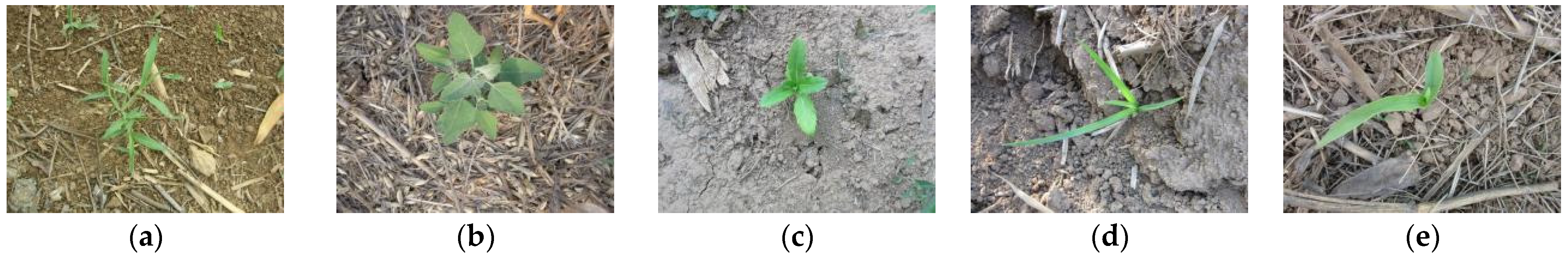
2.3.1. Plant Seedling Dataset

The plant seedling dataset [29] comprises 12 types of crop and weed seedlings, totaling 5539 images. These plant species are common in Denmark and are at different stages of growth. In the experiment, this paper separated these images into a training set and a test set in the ratio of 9:1. Figure 5 randomly shows one photo of each type of seedling.

Table 2. More details of the plant seedling dataset [29].

Class	Species	Training Set	Test Set	Total
1	Black-grass	279	30	309
2	Charlock	407	45	452
3	Cleavers	302	33	335
4	Common chickweed	642	71	713
5	Common wheat	228	25	253
6	Fat hen	485	53	538
7	Loose silky-bent	686	76	762
8	Maize	232	25	257
9	Scentless mayweed	542	60	607
10	Shepherd’s purse	247	27	274
11	Small-flowered cranesbill	519	57	576
12	Sugar beet	417	46	463
Total		4991	548	5539

provides detailed quantity information in the dataset.

2.3.2. Weed–Corn Dataset

The weed–corn dataset [14] is a collection of 5998 images of corn and four weed species (bluegrass, chenopodium album, cirsium setosum, and sedge) on different days and under different light and soil background conditions by Jiang et al. All were individual plant images that were not occluded or covered. After processing, the size of each image was 800 × 600. In the experiment, the ratio of the training set to the test set was 8:2. Figure 6 randomly shows one photo from the weed–corn dataset.

2.3.3. CIFAR-10 Dataset

The CIFAR-10 [30] dataset is a widely accepted computer vision dataset that contains images from 10 different categories (airplane, automobile, bird, cat, deer, dog, frog, horse, ship, and truck), as shown in Figure 7. Each category includes 6000 color images, and each image is saved as 32 × 32 pixels. These images are divided into a training set and a test set, where the training set contains 50,000 images and the test set contains 10,000 images.

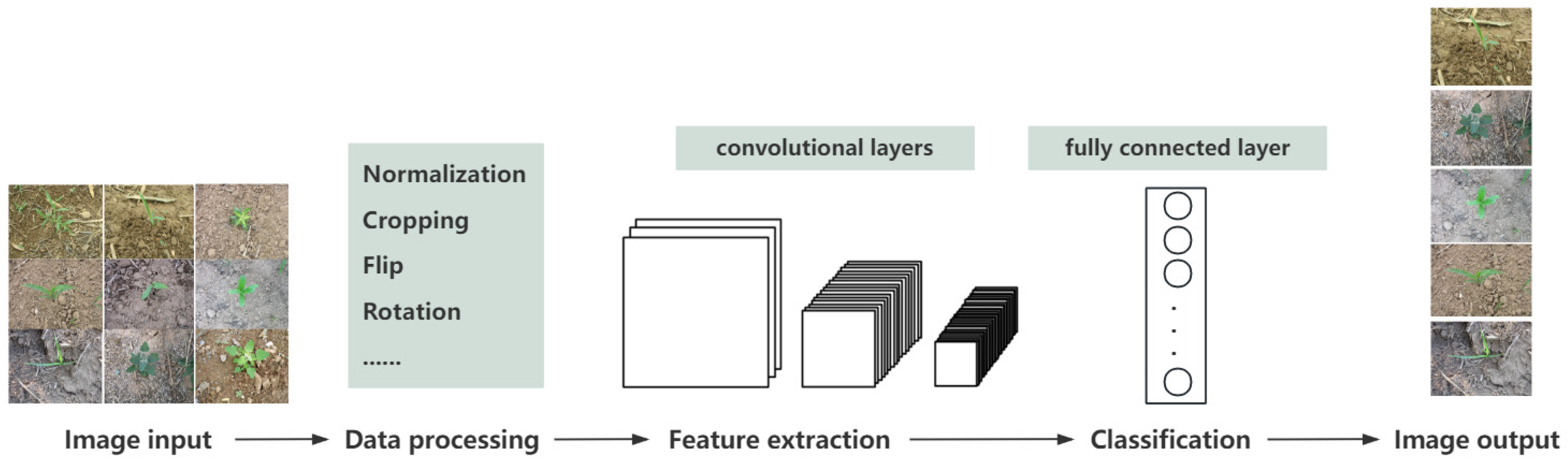
2.3.4. Data Preprocessing and Data Enhancement

Image preprocessing is a critical first step in performing image classification when using deep learning. The most common preprocessing methods include normalization and standardization. Data normalization is the scaling of the image data in equal proportions so that they fall into a specific range of intervals, usually [0, 1] or [−1, 1]. Standardization, however, is transforming the data into a distribution with a mean of 0 and a standard deviation of 1. These two operations can eliminate the scale differences between different eigenvalues, making the model easier to converge.

In network training, overfitting often occurs due to insufficient data [31]. The plant seedling dataset and the weed–corn dataset were augmented with data in this paper. Data augmentation can minimize the influence of poor data size. It can also boost the robustness of the network. It offers a variety of “invariance” for the model and improves the model’s ability to resist overfitting.

Three data enhancement techniques, cropping, flipping, and rotating, were used in this paper.

Cropping: Crop a part of the image randomly or according to certain rules. Commonly used methods are random cropping, cropping from the center of the image, random aspect ratio cropping, etc.

Flip: Flip the image horizontally or vertically. Usually, there are two ways: horizontal flip and vertical flip. This is usually set to a probability of 50% for each of the image flipping and not flipping.

Rotation: The image is rotated at a certain angle to produce more training samples. This data enhancement operation increases the robustness and adaptability of the network to deformation operations, such as rotation and tilt.

3. Experiments and Results

The following experiments were conducted using the PyTorch framework, which is simple, flexible, efficient, and popular for deep learning [32]. The hardware consisted of a PC with a 12th Gen Intel Core i7-12700H CPU and a GeForce RTX 3060 GPU. The development software was Visual Studio Code 1.80, and the programming language was Python 3.10.

Data processing: The plant seedling dataset was used in the first experiment. We adjusted the image data in the dataset to a resolution of 128 × 128, then flipped the images, converted them to Tensor-type data, and normalized them.

The weed–corn dataset was used in the second experiment, and we adjusted the image data in the dataset to a resolution of 128 × 128 and used three data enhancement methods: cropping, flipping, and rotating.

We converted only the CIFAR-10 dataset to Tensor type and normalized it in the third experiment.

Optimizer selection and parameter settings: Stochastic Gradient Descent (SGD) is a gradient-based optimization algorithm for finding parameter configurations that minimize the loss function. SGD updates parameters by calculating the gradient for each sample and randomly selecting one sample or a batch of samples in each update. The steps are as follows: (i) randomly select a training sample, (ii) compute the gradient of that sample, (iii) use the gradient value and the learning rate to update the parameters, and (iv) repeat these steps until the convergence condition is reached or the specified number of iterations is reached.

In these experiments, we used the SGD optimizer to optimize the network with the following parameters: learning rate 0.001, momentum 0.9, weight decay 0.0005, and batch 64.

Cross-validation: Cross-validation is often used to assess the predictive performance of models, which can obtain more effective information from limited data to reduce overfitting to a certain extent and make the results more accurate. In this paper, five-fold cross-validation was used in the training of the plant seedling dataset and the weed–corn dataset.

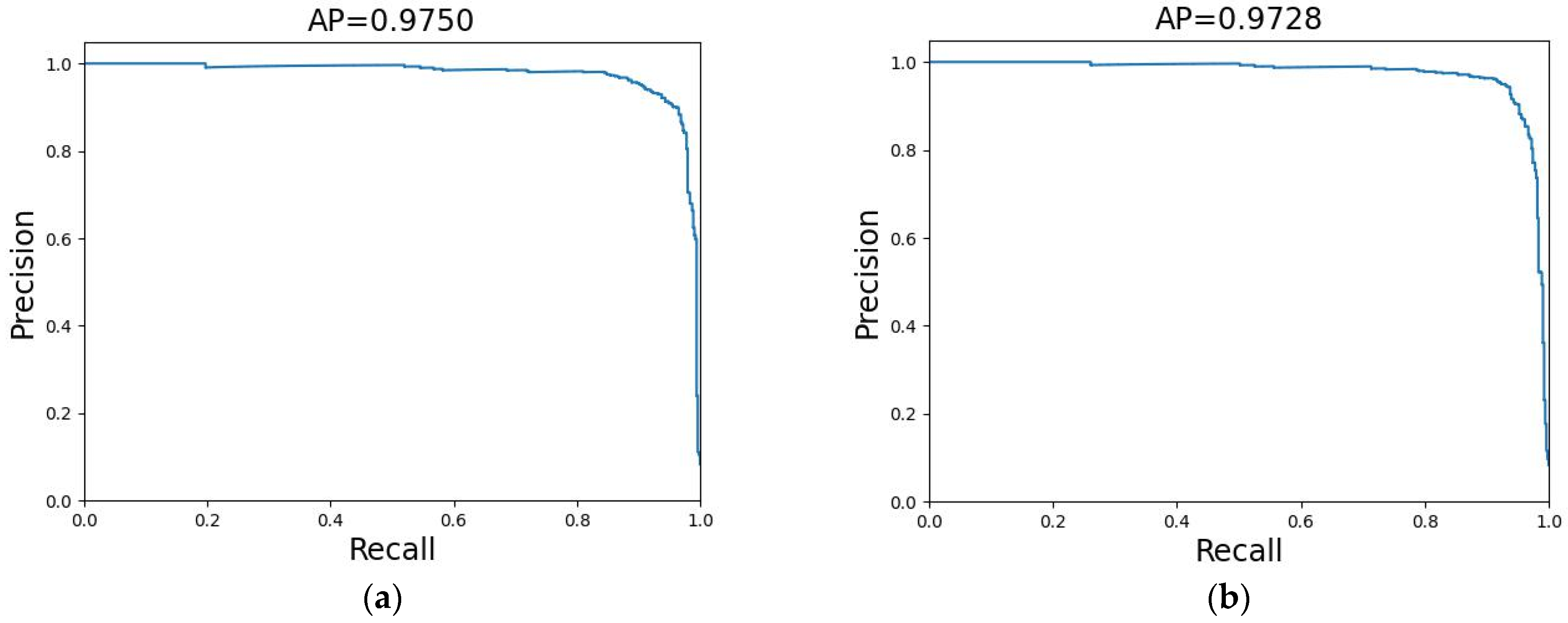
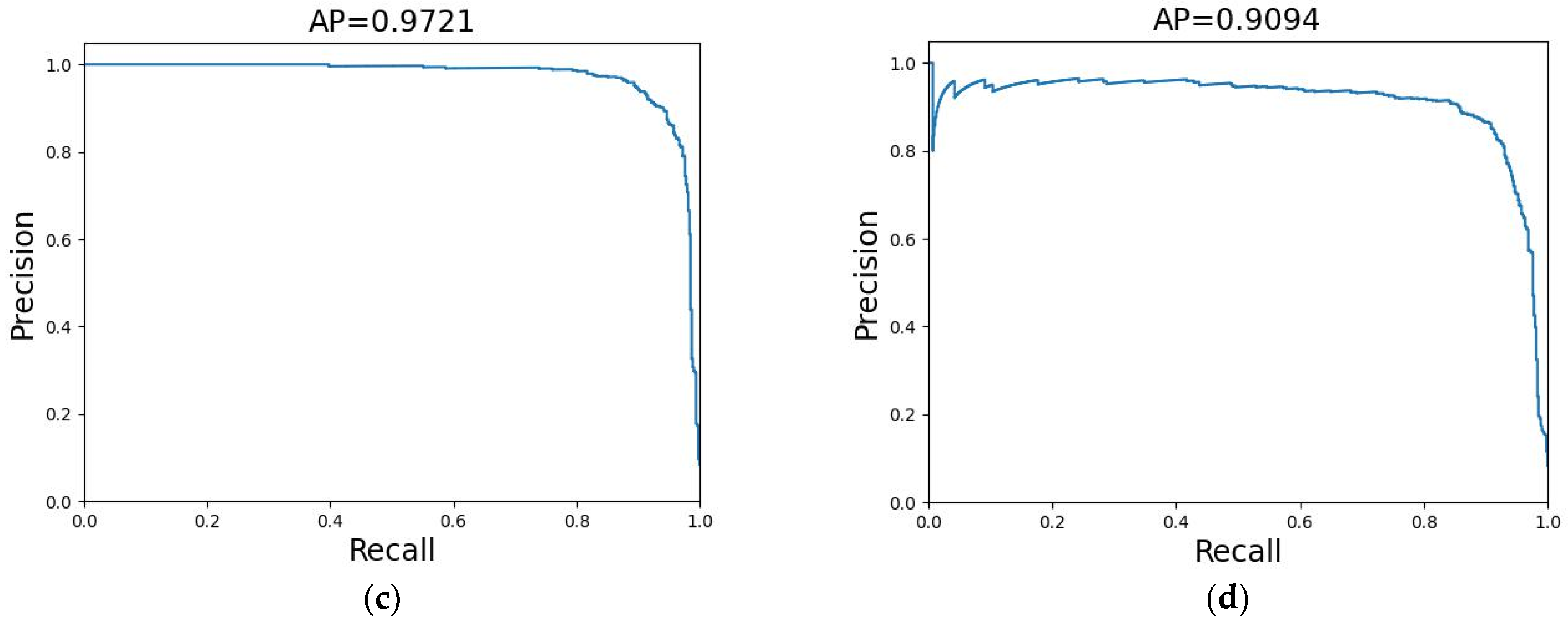
3.1. Results of SkipResNet on the Plant Seedling Dataset

The most commonly used VGG model [33] in CNN-based weed recognition, the representative lightweight network MobileNet model [34], and the ResNet model [26] were selected for experimental comparison with the SkipResNet model proposed in this paper.

In this paper, the plant seeding dataset was divided into the training set and the test set in the ratio of 9:1. Next, a five cross-fold was applied to the training set. A single copy was taken out as the validation set, and the remaining four copies were used as the training set. After several training sessions, the best test results are shown in

Table 3. Results of 5 cross-fold comparison experiments for SkipResNet18, ResNet18, VGG19, and MobileNetV2.

Model	Average Validation Accuracy	Test Accuracy	Test Precision	Test Recall	Test F1	Parameter
SkipResNet18	97.05	95.07	95.05	95.07	95.04	11,184,588
ResNet18	95.97	94.34	94.42	94.34	94.09	11,174,988
VGG19	97.07	94.70	94.74	94.70	94.70	70,418,892
MobileNetV2	93.83	90.32	90.55	90.32	89.96	2,239,244

.

Table 3 shows the average accuracy on the validation set of the four models, SkipResNet18, ResNet18, VGG19, and MobileNetV2, as well as the accuracy, precision, recall, and F1 value on the test set. Although the average accuracy of SkipResNet18 on the validation set was lower than that of VGG19, the performance it showed on the test set was still better than that of the other models. The accuracy of SkipResNet18 was higher than that of ResNet18, VGG19, and MobileNetV2 by 0.73%, 0.37%, and 4.75%, respectively. In terms of parameters, SkipResNet18 has only 9600 more parameters than ResNet18, which is the result of eight more input paths. The number of parameters in VGG19 is almost seven times that of SkipResNet18. Although MobileNetV2 has fewer parameters and is faster to compute, it requires more training rounds to achieve a fit and is less accurate than the other three models. In practical applications, it is critical that the model correctly recognize crops and weeds (positive classes). The higher recall and F1 value in Table 3 indicate the utility and effectiveness of the proposed model.

Figure 8 shows the confusion matrices of SkipResNet18, ResNet18, VGG19, and MobileNetV2 on the plant seedling test set, which visually analyzes how well the networks classify the different categories. SkipResNet18 classified the highest number of plant seedlings correctly into eight categories: black-grass, cleavers, common chickweed, common wheat, fat hen, maize, shepherd’s purse, and small-flowered cranesbill. Although the proposed network model did not show the best performance in all categories, the overall performance of SkipResNet18 was better, as shown in Table 3.

Figure 9 illustrates the precision–recall curve for each model. The AP metric was obtained from the area of the precision–recall curve. Ideally, we would like both precision and recall to be 100%. In other words, the closer the curve is to the upper-right corner, the better it is. However, in real-world applications, there is often a trade-off between the two. Therefore, the AP metric integrates the precision under different recall rates to evaluate the overall performance of the model. The larger the value of AP, the better it represents the model. As can be seen from Figure 9, the AP of SkipResNet18 was 0.9750, which is higher than the AP values of the other models, indicating that the model proposed in this paper has better comprehensive performance.

Table 4. Comparison of accuracy between SkipResNet18 and other state-of-the-art models on the plant seedling dataset.

Model	Accuracy
SkipResNet18 (our method)	95.07
AgroAVNET [35]	93.64
Improved DenseNet(without ECA) [36]	94.34

shows that the SkipResNet18 model had an accuracy 1.43% and 0.73% higher than that of AgroAVNET and Improved DenseNet, respectively, which can prove the classification effectiveness of our model on the plant seedling dataset.

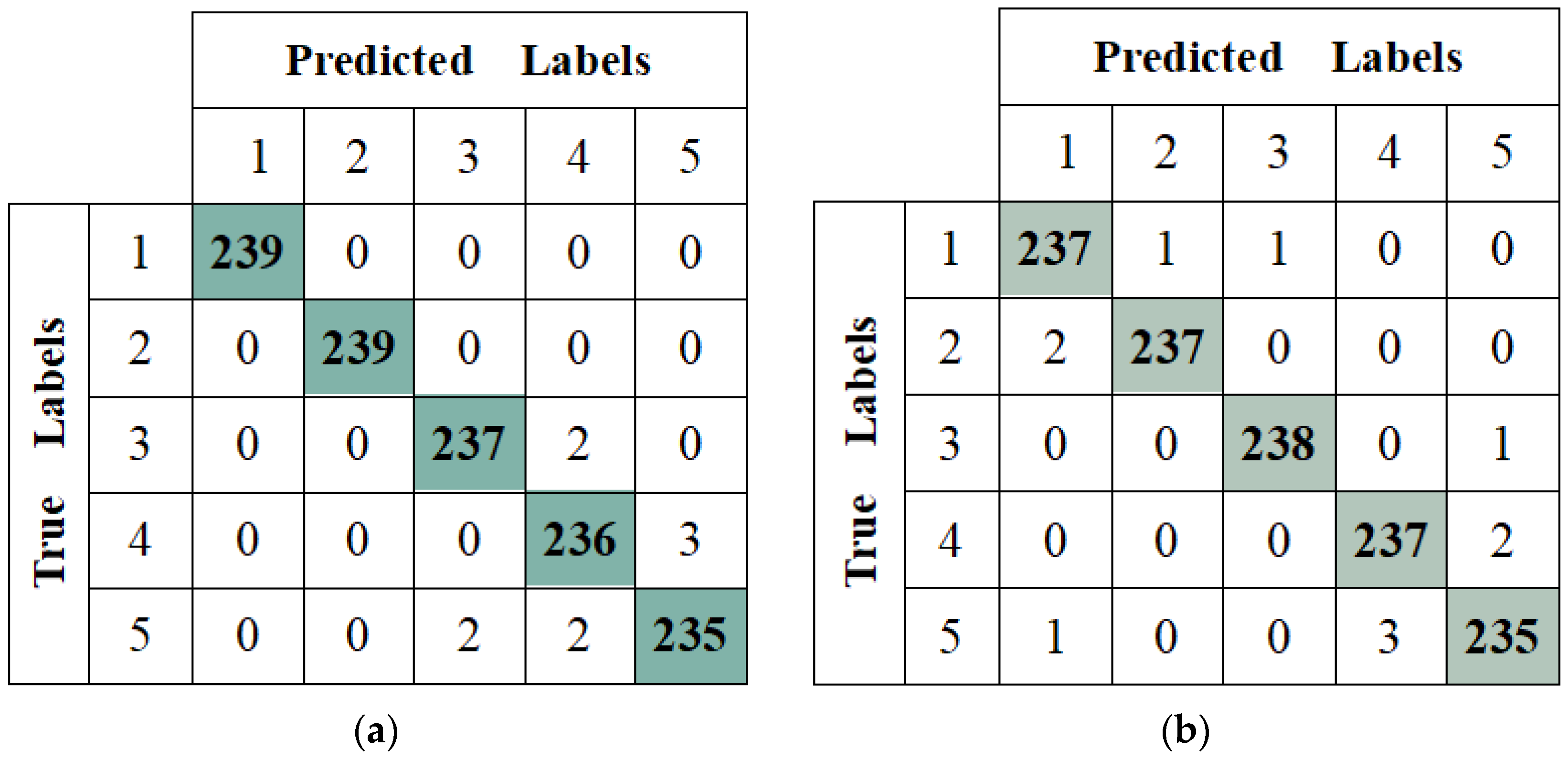
3.2. Results of SkipResNet on the Weed–Corn Dataset

For the sake of verifying the function of SkipResNet in distinguishing between crops and weeds, corn and weed images were evaluated in the test set (239 images for each category). The recognition performance of both SkipResNet18 and ResNet18 algorithms is given in Table 5. It demonstrates that the accuracy, precision, recall, and F1 value of SkipResNet18 were 99.24%, 99.24%, 99.24%, and 99.24%, respectively. Compared to the original ResNet18, the accuracy increased by 0.17%, precision by 0.16%, recall by 0.17%, and the F1 value by 0.17%.

Table 5. Indicator values of SkipResNet18 and ResNet18 on four weeds and corn. The 5 species considered were (1) bluegrass, (2) chenopodium album, (3) cirsium setosum, (4) corn, and (5) sedge.

Class	SkipResNet18				ResNet18
	$\mathbf{Accuracy}$	$\mathbf{P}\mathbf{r}\mathbf{e}\mathbf{c}\mathbf{i}\mathbf{s}\mathbf{i}\mathbf{o}\mathbf{n}$	$\mathbf{Recall}$	$\mathbf{F}1$	$\mathbf{Accuracy}$	$\mathbf{P}\mathbf{r}\mathbf{e}\mathbf{c}\mathbf{i}\mathbf{s}\mathbf{i}\mathbf{o}\mathbf{n}$	$\mathbf{Recall}$	$\mathbf{F}1$
1	100.0	100.0	100.0	100.0	98.75	98.75	99.16	98.95
2	100.0	100.0	100.0	100.0	99.58	99.58	99.16	99.37
3	99.16	99.16	99.16	99.16	99.58	99.58	99.58	99.58
4 (corn)	98.75	98.33	98.74	98.53	98.75	98.75	99.16	98.95
5	98.32	98.73	98.32	98.53	98.73	98.73	98.32	98.53
Average	99.24	99.24	99.24	99.24	99.07	99.08	99.07	99.07

Table 5. Indicator values of SkipResNet18 and ResNet18 on four weeds and corn. The 5 species considered were (1) bluegrass, (2) chenopodium album, (3) cirsium setosum, (4) corn, and (5) sedge.

Class	SkipResNet18				ResNet18
	$\mathbf{Accuracy}$	$\mathbf{P}\mathbf{r}\mathbf{e}\mathbf{c}\mathbf{i}\mathbf{s}\mathbf{i}\mathbf{o}\mathbf{n}$	$\mathbf{Recall}$	$\mathbf{F}1$	$\mathbf{Accuracy}$	$\mathbf{P}\mathbf{r}\mathbf{e}\mathbf{c}\mathbf{i}\mathbf{s}\mathbf{i}\mathbf{o}\mathbf{n}$	$\mathbf{Recall}$	$\mathbf{F}1$
1	100.0	100.0	100.0	100.0	98.75	98.75	99.16	98.95
2	100.0	100.0	100.0	100.0	99.58	99.58	99.16	99.37
3	99.16	99.16	99.16	99.16	99.58	99.58	99.58	99.58
4 (corn)	98.75	98.33	98.74	98.53	98.75	98.75	99.16	98.95
5	98.32	98.73	98.32	98.53	98.73	98.73	98.32	98.53
Average	99.24	99.24	99.24	99.24	99.07	99.08	99.07	99.07

Figure 10. Confusion matrices for SkipResNet18 and ResNet18 on four weed and corn test sets. (a) SkipResNet18 and (b) ResNet18. The 5 species considered were (1) bluegrass, (2) chenopodium album, (3) cirsium setosum, (4) corn, and (5) sedge.

Figure 10. Confusion matrices for SkipResNet18 and ResNet18 on four weed and corn test sets. (a) SkipResNet18 and (b) ResNet18. The 5 species considered were (1) bluegrass, (2) chenopodium album, (3) cirsium setosum, (4) corn, and (5) sedge.

Figure 10 displays the confusion matrices for two models. It fully illustrates the categorization of each class of plants. As shown in Figure 10, bluegrass and chenopodium album were classified correctly using the SkipResNet18 algorithm. Although ResNet18 performed a little better on cirsium setosum and corn, overall, the number of SkipResNet18 classification errors was 9, and the number of ResNet18 classification errors was 11.

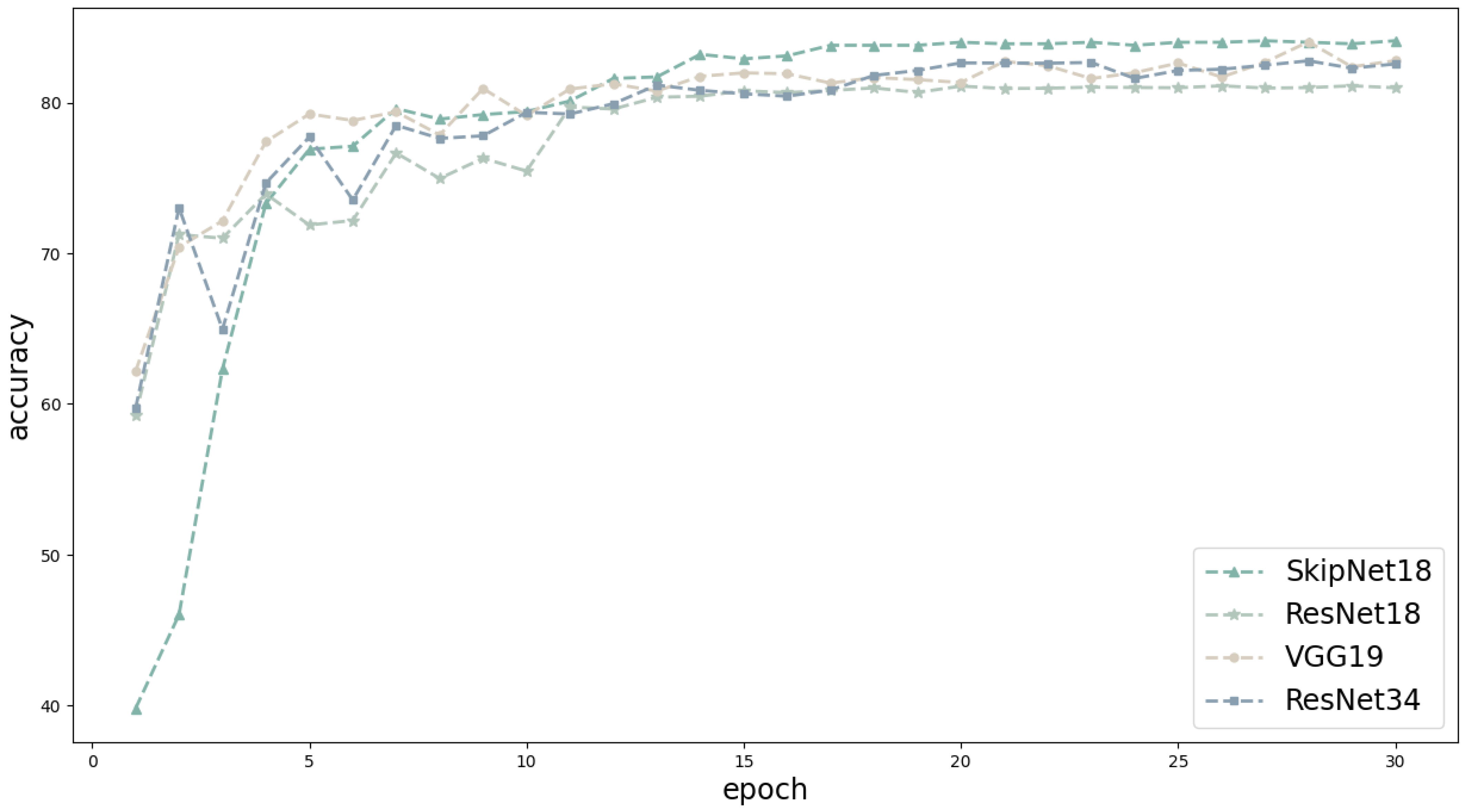
3.3. Results of SkipNet on the CIFAR-10 Dataset

With a view to proving the validity and generalizability of the path selection approach and the multi-path input network proposed in this paper, we evaluated SkipNet18 using CIFAR-10, a classical dataset, when performing image classification. Furthermore, comparative experiments were conducted with classical network models. The model accuracy is shown in Figure 11.

Figure 11 illustrates the classification accuracy plots of SkipNet18, ResNet18, VGG19, and ResNet34 models after multiple trials without data enhancement. As can be seen in Figure 11, SkipNet18 was more accurate than the other models from epoch 13 onward. With the same number of network layers, the 18-layer SkipNet was 3.3% superior to the 18-layer ResNet. When the network depths were different, the 18-layer SkipNet was 1.7% better than the 34-layer ResNet model and 1.5% better than the 19-layer VGG.

In

Table 6. Precision, recall, F1 value, and number of parameters for SkipNet18, ResNet18, VGG19, and ResNet34 on the CIFAR-10 dataset.

Model	Accuracy	$\mathbf{P}\mathbf{r}\mathbf{e}\mathbf{c}\mathbf{i}\mathbf{s}\mathbf{i}\mathbf{o}\mathbf{n}$	Recall	F1	Parameter
SkipNet18	84.3	84.2	84.3	84.2	11,019,673
ResNet18	81.0	80.7	81.0	80.8	11,173,962
VGG19	82.8	83.0	82.8	82.8	38,953,418
ResNet34	82.6	82.6	82.6	82.5	21,282,122

, from the point of view of precision, recall, and the F1 value, SkipNet18 was shown to outperform the other three high-performance network models in image classification. SkipNet18 had 154,289 fewer parameters than ResNet18, which has the same number of layers. This shows that the proposed network architecture can realize superior performance with fewer parameters.

In summary, the effectiveness and generalizability of the path selection algorithm and the multi-path input network proposed in this paper for image classification are demonstrated.

4. Discussion

Weeds compete with crops for soil nutrients, sunlight, etc., and they grow fast, leading to a substantial compression of crop growth space. So, weeds have a serious inhibitory effect on crop yield. Weeds are extremely harmful to crops and must be controlled and treated in a timely manner [37]. Among the many methods of weed control and protection, chemical weed control has become the main way of weed control in the field at home and abroad [38]. Chemical weed control can eliminate 90–99% of inter- and intra-row weeds. However, excessive use of chemical herbicides can pollute soil and groundwater and pose a threat to the diversity of farmland ecosystems. With the concept of smart agriculture, precision weed control using smart machinery has become an important research direction. To realize automated weed removal technology, the initial challenge is to accurately identify and classify weeds and crops. There are three common field weed identification methods: manual identification, remote sensing identification, and machine-vision-based identification [39]. Machine-vision-based recognition methods are the mainstay of plant recognition research, and these methods are highly accurate, fast, and labor saving.

Image data are widely present in life and various fields. With increasing complexity, data analysis and processing have become increasingly difficult. Deep learning has received widespread attention since it was proposed, and its continuous perfecting and development have led to a dramatic improvement in image classification and recognition. On the one hand, image classification models can now be trained on sizable datasets. On the other hand, they can extract high-level features in image data that better characterize the content of the images. Thus, they have significant advantages in solving image classification problems. Currently, CNN-based recognition methods show the best advantage in weed and crop classification.

ResNet allows information in the network to be passed across multiple layers, and the network can then learn features at a deeper level. We envisioned the possibility of combining ResNet with path selection algorithms and proposed an 18-layer multi-path input skip-residual neural network with nine input paths. We applied this new network to the recognition of weeds and crops. From the perspective of accuracy, SkipResNet18 was 0.73% better than ResNet18, with the same number of layers. SkipResNet18 also performed better than ResNet18 in the corn–weed dataset. However, we observe from Figure 10 that there are still some cases of misclassification of seedlings. This may be due to the fact that corn seedlings and sedge seedlings are too similar or that the hierarchy of our proposed network is not deep enough, because the dataset is not large.

Finally, in order to explore whether the multi-path input and path selection algorithms designed can be implemented on other image classifications, we evaluated them using the CIFAR-10 dataset. The final experimental results illustrate that the multi-path input and path selection algorithms are feasible.

In addition to weed recognition, the CNN can be seen in other agricultural areas as well, for instance, rose flower classification [40], strawberry ripeness detection [41], plant pests and diseases [42], and plant leaf counting [43]. The results on the CIFAR-10 dataset show that our proposed new model can be applied to other agricultural image recognition.

In this research, the information generated in the intermediate layer of deep neural networks was explored so that the information can be fully used. The multi-path input no longer limits the data input to the initial layer, and the network’s structure has become more flexible. The same network model may have differences in the focus area of attention for different categories of images, and images may have preferences for different layers of the same network model, i.e., images in different categories may achieve optimal accuracy under different input paths. In other words, under the same network model, each category can find an input path suitable for its own image features.

In training and testing, we found that SkipResNet takes about twice as long as ResNet per round. This is because the image data first traverse all the paths so as to select a path that best suits them. However, in the current development of intelligent weeding robots, in addition to high efficiency, real-time performance is a key point. SkipResNet, as proposed in this paper, however, does not have an advantage in terms of real-time performance. In addition, since the dataset we used is publicly available and has been processed, we cannot confirm whether our proposed model can show good recognition performance under the variable and complex real scenarios in the field. This will be the direction of our future research.

5. Conclusions

In this paper, a neural network with multi-path inputs was proposed to improve image classification performance. In terms of network structure improvement, we added multiple input paths to enhance the flexibility of the network architecture and discussed the use of the information generated in the intermediate layer of the neural network. In addition, this paper constructed three path selection algorithms for multi-path input neural networks. The first path selection method is the minimum loss value path selection algorithm. Image data are input into the network from different paths, and the path with the lowest loss value among all the paths is selected as the optimal path. The second path selection algorithm is the individual optimal path selection algorithm. For each data item in a batch, its optimal path is selected and input into the network for computation. The third path selection algorithm is the optimal path statistical selection algorithm. For all the image data in a batch, the optimal paths they selected are counted and the one with the highest number of selections is used as the path selection for the whole batch to obtain the final prediction. The three algorithms are used together, which can promote the convergence speed as well as the comprehensive performance.

A multi-path input skip-residual network was proposed by combining the ResNet model with a path selection algorithm. On the plant seedling dataset, which contains three types of crops and nine types of weeds, SkipResNet18 improved the recognition accuracy by 0.73% and 0.37% compared to ResNet18 and VGG19, respectively. SkipResNet18 also showed better performance than ResNet18 on the corn–weed dataset. A new neural network research method was proposed for the fields of UAV low-altitude spraying, precision agriculture, and smart agriculture, which can more accurately recognize different kinds of crops and weeds, prevent the misuse of pesticides, and protect the ecosystem.

On the CIFAR-10 dataset, the empirical results demonstrated that the network model proposed has excellent classification effects and scalability. It provides a new research idea for CNN algorithm improvement.

However, our network model still has some shortcomings: we used three path selection algorithms, so the training time was longer than the general model. Due to our hardware, we did not perform experimental analyses on larger datasets and in real field environments.

From the literature [36], we find that adding an attention mechanism can greatly improve the recognition accuracy of the network. Our future work will attempt to incorporate the attention mechanism to continue to improve the performance of our network. In addition, we will explore whether our proposed algorithms can be effectively combined with lightweight networks, which in turn can reduce the training and testing time to meet the real-time requirements in real applications. Furthermore, for future research, we should also focus on the adaptability and robustness of the model in real field environments. It is hoped that through our continuous optimization and improvement, we can achieve better weed image classification results, which will lead to smarter and safer use of herbicides, reduce land pollution, and protect the ecological environment and ensure food security.

References

1. Zhang, Z.; Liu, H.; Meng, Z.; Chen, J. Deep learning-based automatic recognition network of agricultural machinery images. Comput. Electron. Agric. 2019, 166, 104978. [Google Scholar] [CrossRef]
2. Yang, K.; Liu, H.; Wang, P.; Meng, Z.; Chen, J. Convolutional neural network-based automatic image recognition for agricultural machinery. Int. J. Agric. Biol. Eng. 2018, 11, 200–206. [Google Scholar] [CrossRef]
3. Adve, V.; Wedow, J.; Ainsworth, E.; Chowdhary, G.; Green-Miller, A.; Tucker, C. AIFARMS: Artificial intelligence for future agricultural resilience, management, and sustainability. AI Mag. 2024, 45, 83–88. [Google Scholar] [CrossRef]
4. Sun, T.; Cui, L.; Zong, L.; Zhang, S.; Jiao, Y.; Xue, X.; Jin, Y. Weed Recognition at Soybean Seedling Stage Based on YOLOV8nGP+ NExG Algorithm. Agronomy 2024, 14, 657. [Google Scholar] [CrossRef]
5. Jiang, W.; Quan, L.; Wei, G.; Chang, C.; Geng, T. A conceptual evaluation of a weed control method with post-damage application of herbicides: A composite intelligent intra-row weeding robot. Soil Tillage Res. 2023, 234, 105837. [Google Scholar] [CrossRef]
6. Sheela, J.; Karthika, N.; Janet, B. SSLnDO-Based Deep Residual Network and RV-Coeącient Integrated Deep Fuzzy Clustering for Cotton Crop Classification. Int. J. Inf. Technol. Decis. Mak. 2024, 23, 381–412. [Google Scholar]
7. Zheng, Y.; Zhu, Q.; Huang, M.; Guo, Y.; Qin, J. Maize and weed classification using color indices with support vector data description in outdoor fields. Comput. Electron. Agric. 2017, 141, 215–222. [Google Scholar] [CrossRef]
8. Sajad, S.; Yousef, A.; Juan, I. An automatic visible-range video weed detection, segmentation and classification prototype in potato field. Heliyon 2020, 6, e03685. [Google Scholar]
9. Adel, B.; Abdolabbas, J. Evaluation of support vector machine and artificial neural networks in weed detection using shape features. Comput. Electron. Agric. 2018, 145, 153–160. [Google Scholar]
10. Kounalakis, T.; Triantafyllidis, G.A.; Nalpantidis, L. Weed recognition framework for robotic precision farming. In Proceedings of the 2016 IEEE International Conference on Imaging Systems and Techniques (IST), Chania, Greece, 4–6 October 2016; pp. 466–471. [Google Scholar]
11. Bakhshipour, A.; Jafari, A.; Nassiri, S.M.; Zare, D. Weed segmentation using texture features extracted from wavelet sub-images. Biosyst. Eng. 2017, 157, 1–12. [Google Scholar] [CrossRef]
12. Le, V.N.T.; Apopei, B.; Alameh, K. Effective plant discrimination based on the combination of local binary pattern operators and multiclass support vector machine methods. Inf. Process. Agric. 2019, 6, 116–131. [Google Scholar]
13. Sun, Y.; Chen, Y.; Jin, X.; Yu, J.; Chen, Y. An artificial intelligence-based method for recognizing seedlings and weeds in Brassica napus. Fujian J. Agric. Sci. 2021, 36, 1484–1490. [Google Scholar]
14. Jiang, H.; Zhang, C.; Qiao, Y.; Zhang, Z.; Zhang, W.; Song, C. CNN feature based graph convolutional network for weed and crop recognition in smart farming. Comput. Electron. Agric. 2020, 174, 105450. [Google Scholar] [CrossRef]
15. Cecili, G.; De Fioravante, P.; Dichicco, P.; Congedo, L.; Marchetti, M.; Munafò, M. Land Cover Mapping with Convolutional Neural Networks Using Sentinel-2 Images: Case Study of Rome. Land 2023, 12, 879. [Google Scholar] [CrossRef]
16. Tao, T.; Wei, X. A hybrid CNN–SVM classifier for weed recognition in winter rape field. Plant Methods 2022, 18, 29. [Google Scholar] [CrossRef] [PubMed]
17. Liu, Y.; Xue, J.; Li, D.; Zhang, W.; Chiew, T.; Xu, Z. Image recognition based on lightweight convolutional neural network: Recent advances. Image Vis. Comput. 2024, 146, 105037. [Google Scholar] [CrossRef]
18. Dyrmann, M.; Karstoft, H.; Midtiby, H. Plant species classification using deep convolutional neural network. Biosyst. Eng. 2016, 151, 72–80. [Google Scholar] [CrossRef]
19. dos Santos Ferreira, A.; Freitas, D.M.; da Silva, G.G.; Pistori, H.; Folhes, M.T. Weed detection in soybean crops using ConvNets. Comput. Electron. Agric. 2017, 143, 314–324. [Google Scholar] [CrossRef]
20. Zhang, L.; Jin, X.; Fu, L.; Li, S. Recognition method for weeds in rapeseed field based on Faster R-CNN deep network. Laser Optoelectron. Prog. 2020, 57, 304–312. [Google Scholar] [CrossRef]
21. Garibaldi-Márquez, F.; Flores, G.; Mercado-Ravell, D.A.; Ramírez-Pedraza, A.; Valentín-Coronado, L.M. Weed Classification from Natural Corn Field-Multi-Plant Images Based on Shallow and Deep Learning. Sensors 2022, 22, 3021. [Google Scholar] [CrossRef] [PubMed]
22. Luo, T.; Zhao, J.; Gu, Y.; Zhang, S.; Qiao, X.; Tian, W.; Han, Y. Classification of weed seeds based on visual images and deep learning. Inf. Process. Agric. 2023, 10, 40–51. [Google Scholar] [CrossRef]
23. Babu, V.S.; Ram, N.V. Deep residual CNN with contrast limited adaptive histogram equalization for weed detection in soybean crops. Trait. Signal 2022, 39, 717–722. [Google Scholar] [CrossRef]
24. Manikandakumar, M.; Karthikeyan, P. Weed classification using particle swarm optimization and deep learning models. Comput. Syst. Sci. Eng. 2023, 44, 913–927. [Google Scholar] [CrossRef]
25. Xu, K.; Yuen, P.; Xie, Q.; Zhu, Y.; Cao, W.; Ni, J. WeedsNet: A dual attention network with RGB-D image for weed detection in natural wheat field. Precis. Agric. 2024, 25, 460–485. [Google Scholar] [CrossRef]
26. He, K.; Zhang, X.; Ren, S.; Sun, J. Deep residual learning for image recognition. In Proceedings of the 2016 IEEE Conference on Computer Vision and Pattern Recognition (CVPR), Las Vegas, NV, USA, 27–30 June 2016; pp. 770–778. [Google Scholar]
27. Feng, Z.; Ji, H.; Daković, M.; Cui, X.; Zhu, M.; Stanković, L. Cluster-CAM: Cluster-weighted visual interpretation of CNNs’ decision in image classification. Neural Netw. 2024, 178, 106473. [Google Scholar] [CrossRef] [PubMed]
28. Krstinić, D.; Skelin, A.; Slapničar, I.; Braović, M. Multi-Label Confusion Tensor. IEEE Access 2024, 12, 9860–9870. [Google Scholar] [CrossRef]
29. Giselsson, T.M.; Jørgensen, R.; Jensen, P.; Dyrmann, M.; Midtiby, H. A Public Image Database for Benchmark of Plant Seedling Classification Algorithms. arXiv 2017, arXiv:1711.05458. [Google Scholar]
30. Krizhevsky, A. Learning Multiple Layers of Features from Tiny Images. Master’s Thesis, University of Toronto, Toronto, ON, Canada, 2009. [Google Scholar]
31. Li, H.; Rajbahadur, G.; Lin, D.; Bezemer, C.; Jiang, Z. Keeping Deep Learning Models in Check: A History-Based Approach to Mitigate Overfitting. IEEE Access 2024, 12, 70676–70689. [Google Scholar] [CrossRef]
32. Song, Y.; Zou, Y.; Li, Y.; He, Y.; Wu, W.; Niu, R.; Xu, S. Enhancing Landslide Detection with SBConv-Optimized U-Net Architecture Based on Multisource Remote Sensing Data. Land 2024, 13, 835. [Google Scholar] [CrossRef]
33. Simonyan, K.; Zisserman, A. Very deep convolutional networks for large-scale image recognition. arXiv 2015, arXiv:1409.1556. [Google Scholar]
34. Howard, A.G.; Zhu, M.; Chen, B.; Kalenichenko, D.; Wang, W.; Weyand, T.; Andreetto, M.; Adam, H. MobileNets: Efficient convolutional neural networks for mobile vision applications. arXiv 2017, arXiv:1704.04861. [Google Scholar]
35. Chavan, T.R.; Nandedkar, A.V. AgroAVNET for crops and weeds classification: A step forward in automatic farming. Comput. Electron. Agric. 2018, 154, 361–372. [Google Scholar] [CrossRef]
36. Mu, Y.; Ni, R.; Fu, L.; Luo, T.; Feng, R.; Li, J.; Li, S. DenseNet weed recognition model combining local variance preprocessing and attention mechanism. Front. Plant Sci. 2023, 13, 1041510. [Google Scholar] [CrossRef] [PubMed]
37. Qu, H.; Su, W. Deep Learning-Based Weed–Crop Recognition for Smart Agricultural Equipment: A Review. Agronomy 2024, 14, 363. [Google Scholar] [CrossRef]
38. Søgaard, H.T.; Lund, I.; Graglia, E. Real-time application of herbicides in seed lines by computer vision and micro-spray system. In Proceedings of the 2006 ASAE Annual Meeting, Portland, Oregon, 9–12 July 2006; American Society of Agricultural and Biological Engineers: St. Joseph, MI, USA, 2006. [Google Scholar]
39. Qu, F.; Li, W.; Yang, Y.; Liu, H.; Hao, Z. Crop weed recognition based on image enhancement and attention mechanism. Comput. Eng. Des. 2023, 44, 815–821. [Google Scholar]
40. Wang, X.Y.; Zhang, C.; Zhang, L. Recognition of similar rose based on convolution neural network. J. Anhui Agric. Univ. 2021, 48, 504–510. [Google Scholar]
41. Chen, Y.; Xu, H.; Chang, P.; Huang, Y.; Zhong, F.; Jia, Q.; Chen, L.; Zhong, H.; Liu, S. CES-YOLOv8: Strawberry Maturity Detection Based on the Improved YOLOv8. Agronomy 2024, 14, 1353. [Google Scholar] [CrossRef]
42. Xiong, H.; Li, J.; Wang, T.; Zhang, F.; Wang, Z. EResNet-SVM: An overfitting-relieved deep learning model for recognition of plant diseases and pests. J. Sci. Food Agric. 2024, 104, 6018–6034. [Google Scholar] [CrossRef] [PubMed]
43. Deb, M.; Dhal, K.G.; Das, A.; Hussien, A.G.; Abualigah, L.; Garai, A. A CNN-based model to count the leaves of rosette plants (LC-Net). Sci. Rep. 2024, 14, 1496. [Google Scholar] [CrossRef] [PubMed]
Figure 1. General description of the methodology for weed classification.
Land 13 01585 g001
Figure 2. Structure of a residual block: x is the data input to layer1, F(x) is the output after the data are computed by layer1 and layer2, and there is a skip connection between x and F(x) such that the output of the residual block becomes x + F(x).
Land 13 01585 g002
Figure 3. Improvement of residual blocks: x is the data input of ayer1 (the output of the layer before layer 1 in the network), x0 are the original input data, and F(x) is the output after the computation of layer1 and layer2. After deriving F(x), x0 is re-inputted so that the output of the residual block is changed to x0 + F(x).
Land 13 01585 g003
Figure 4. The framework of ResNet, SkipResNet, and SkipNet. (a) The 18-layer ResNet, which is equivalent to the 18-layer SkipResNet when k = 1; (b) the 18-layer SkipResNet, which shows the first input in the middle layer of the path (k = 2); (c) the 18-layer SkipResNet, with the figure showing the second input path at the middle layer (k = 3); and (d) evaluation of the 18-layer SkipNet for the CIFAR-10 dataset, with an input image resolution of 32 × 32. Here, k is the input path labeling.
Land 13 01585 g004aLand 13 01585 g004b
Figure 5. Example images of the plant seedling dataset [29]. The labels in this figure correspond to the labels in Table 2. (a) Black-grass, (b) charlock, (c) cleavers, (d) common chickweed, (e) common wheat, (f) fat hen, (g) loose silky-bent, (h) maize, (i) scentless mayweed, (j) shepherd’s purse, (k) small-flowered cranesbill, and (l) sugar beet.
Land 13 01585 g005
Figure 6. Weed–corn dataset [14]: (a) bluegrass, (b) chenopodium album, (c) cirsium setosum, (d) sedge, and (e) corn.
Land 13 01585 g006
Figure 7. CIFAR-10 dataset [30].
Land 13 01585 g007
Figure 8. Confusion matrices of SkipResNet18, ResNet18, VGG19, and MobileNetV2 on a test set of 12 plant seedlings: (a) SkipResNet18; (b) ResNet18; (c) VGG19; (d) MobileNetV2. The 12 species considered were (1) black-grass, (2) charlock, (3) cleavers, (4) common chickweed, (5) common wheat, (6) fat hen, (7) loose silky-bent, (8) maize, (9) scentless mayweed, (10) shepherd’s purse, (11) small-flowered cranesbill, and (12) sugar beet.
Land 13 01585 g008aLand 13 01585 g008b
Figure 9. Precision–recall plots for (a) SkipResNet18, (b) ResNet18, (c) VGG19, and (d) MobileNetV2.
Land 13 01585 g009aLand 13 01585 g009b
Figure 11. Accuracy of SkipNet18, ResNet18, VGG19, and ResNet34 models on the CIFAR-10 dataset.
Land 13 01585 g011