Article

Assessment of Carbon Stock and Sequestration Dynamics in Response to Land Use and Land Cover Changes in a Tropical Landscape

1
Department of Geography, Vidyasagar University, Midnapore 721102, India
2
RS-GIS Laboratory, Environmental Technology Division, CSIR-Institute of Himalayan Bioresource Technology, Palampur 176061, India
3
Department of Civil Engineering, College of Engineering, King Saud University, P.O. Box 800, Riyadh 11421, Saudi Arabia
4
Institute of Geospatial Engineering and Geodesy, Faculty of Civil Engineering and Geodesy, Military University of Technology, 00-908 Warsaw, Poland
5
Public Works Engineering Department, Faculty of Engineering, Mansoura University, Mansoura 35516, Egypt
*
Author to whom correspondence should be addressed.
Land 2024, 13(10), 1689; https://doi.org/10.3390/land13101689
Submission received: 23 August 2024 / Revised: 12 October 2024 / Accepted: 14 October 2024 / Published: 16 October 2024

Abstract

:
Quantitative analysis of LULC changes and their effects on carbon stock and sequestration is important for mitigating climate change. Therefore, this study examines carbon stock and sequestration in relation to LULC changes using the Land Change Modeler (LCM) and Ecosystem Services Modeler (ESM) in tropical dry deciduous forests of West Bengal, India. The LULC for 2006, 2014, and 2021 were classified using Google Earth Engine (GEE), while LULC changes and predictions were analyzed using LCM. Carbon stock and sequestration for present and future scenarios were estimated using ESM. The highest carbon was stored in forest land (124.167 Mg/ha), and storage outside the forest declined to 13.541 Mg/ha for agricultural land and 0–8.123 Mg/ha for other lands. Carbon stock and economic value decreased from 2006 to 2021, and are likely to decrease further in the future. Forest land is likely to contribute to 94% of future carbon loss in the study region, primarily due to its conversion into agricultural land. The implementation of multiple-species plantations, securing tenure rights, proper management practices, and the strengthening of forest-related policies can enhance carbon stock and sequestration. These spatial-temporal insights will aid in management strategies, and the methodology can be applied to broader contexts.

1. Introduction

Since the Industrial Revolution, the concentration of greenhouse gasses has been increasing, with a particularly accelerated rate of increase in the past two to five decades [1]. The levels of the three primary greenhouse gasses (GHGs) in the atmosphere are presently greater than any recorded values in the past 800,000 years, and in 2019, the concentrations of methane (CH4), carbon dioxide (CO2), and nitrous oxide (N2O) reached 1866.3 parts per billion (ppb), 409.9 parts per million (ppm), and 332.1 ppb, respectively [2]. Among the GHGs, CO2 alone contributes almost 77% of the total GHG emissions from human activities, which is responsible for approximately 56% of the global warming potential [3]. The concentration of CO2 in the atmosphere has been increasing from a pre-industrial level of 279 parts per million by volume (ppmv) to 409.9 ppmv in 2019. Furthermore, current atmospheric CO2 concentrations are unprecedented relative to the last 2 million years [2].
There are two anthropogenic sources of CO2: combustion of fossil fuels and net emissions from land use change and land management (also known as LULUCF: Land Use, Land Use Change, and Forestry) [2]. The CO2 released from these (fossil fuels and LULUCF) anthropogenic sources between 2010 and 2019 (decadal average 10.9 ± 0.9 PgC/year) was distributed among three components of the Earth system: 46% of it was accumulated in the atmosphere (5.1 ± 0.02 PgC/year), 23% was absorbed by the ocean (2.5 ± 0.6 PgC/year), and 31% was sequestered by vegetation (LULC) (3.4 ± 0.9 PgC/year) [2]. Thus, land use land cover in terrestrial ecosystems has a significant effect on carbon stock and sequestration over a landscape [4,5]. Additionally, LULC changes and their effects on carbon stock and sequestration vary across different regions [6]. So, it is important to investigate carbon stock and sequestration in relation to the LULC types in different regions of terrestrial ecosystems.
In terrestrial ecosystems, forests alone store up to 80% of all above-ground carbon and up to 40% of all below-ground carbon across the globe [7,8]. Among the world’s forests, tropical forests alone store approximately 40% of the total terrestrial carbon [9,10], and have significant impacts on climate change [11,12]. They store about 428 Pg of carbon, with vegetation storing nearly 58%, soil 41%, and litter 1% [13]. Additionally, tropical forests play a crucial role in global net primary productivity, making them one of the most productive ecosystems on the planet [14]. But tropical forests are experiencing a greater reduction in forest cover, or a conversion of forests to other land uses [15]. Tropical forests are exploited for different purposes, including shifting cultivation, for pastures, logging, agricultural expansion, tree plantations, and fires [16]. Land clearing for agriculture is the primary driver of forest loss in tropical countries [17], followed by infrastructure development and wood extraction [18]. These changes in LULC are significant in affecting carbon stock and sequestration in a particular region [4]. Despite their importance and vulnerability, tropical forests have been relatively under-sampled, meaning that our understanding of their carbon dynamics is incomplete [10].
Several studies [4,19,20] have assessed in carbon stock and sequestration in relation to the LULC types using the Integrated Valuation of Ecosystem Services and Tradeoffs (InVEST) model. A few studies analyzed the economic value of carbon [4,21]. The economic value of any ecosystem service is important for increasing awareness and evaluating the importance of a particular service [21,22]. Previous studies primarily used the Land Change Modeler (LCM) in TerrSet for LULC change and prediction analysis, while carbon stock and sequestration with economic value were assessed using the InVEST model [4]. Preparing data according to the requirements of these two software programs and transferring raster data from TerrSet to InVEST is always a time-consuming process and requires expertise in both types of software. The TerrSet 2020 (version 19) Geospatial Monitoring and Modelling System has recently developed Ecosystem Services Modeler (ESM), which provides 15 models, including carbon stock and sequestration (https://clarklabs.org/: accessed on 12 March 2023). Therefore, analyzing ecosystem services can be easier with the integration of ESM and LCM in TerrSet. By using LCM, users can simulate LULC changes in present and future scenarios, and then ESM can be used to quantify the changes in ecosystem services due to LULC changes. Overall, the availability of both LCM and ESM in TerrSet can make it easier for researchers to switch between the modules and can provide a more streamlined and efficient workflow.
The tropical dry deciduous forests of West Bengal play a significant role in the livelihoods of the people [23], but the demands of an enormous population are leading to an increase in natural forest loss in the recent period and forest land being converted to other land types in this region, resulting in negative effects on ecosystem services [24]. But, no previous studies have focused on the carbon stocks and sequestrations in different LULC types in this region. Therefore, we analyzed carbon stocks and sequestrations, along with economic valuation in present and future scenarios in different LULC types. Thus, the objectives of the study are set as: (1) to evaluate the LULC change in present and future scenarios using LCM; and (2) to measure the carbon stocks and sequestrations, along with economic valuation, in present and future scenarios in different LULC types using ESM.

2. Materials and Methods

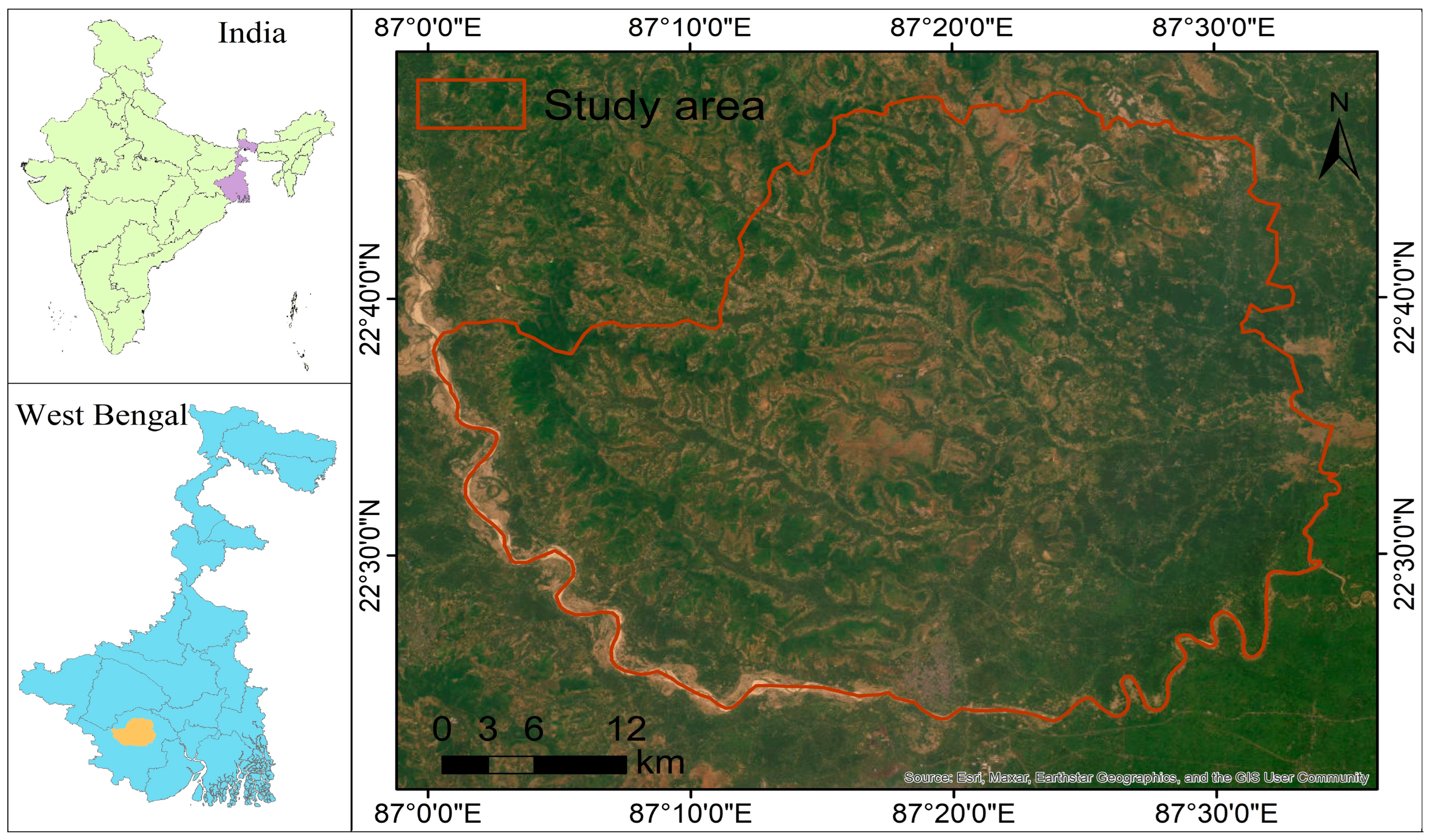
2.1. Descriptions of the Study Area

The southwestern region of West Bengal, India, is known for its fragmented forest cover due to human encroachments [24,25]. We selected the Midnapore forest division of the southwestern region for this study, which extends from 22°23′31″ N to 22°47′59″ N and 87°0′13″ E to 87°34′42″ E (Figure 1). The study area covers an area of about 1822.91 km2, with forest land accounting for approximately 24.85% of the total study area [26]. The forests are tropical dry deciduous, and are characterized by the prevalence of tree species such as Shorea robusta, Acacia auriculiformis, Anacardium occidentale, Diospyros melanoxylon, Terminalia bellirica, Tectona grandis, Madhuca longifolia, and Albizia lebbeck [27]. The climate is AW (Tropical savanna) with a yearly rainfall of 1502.8 mm, an average temperature of 27 °C, and a relative humidity range of 63% (February) to 81% (September) (https://www.timeanddate.com: accessed on 12 March 2023). In terms of topography, the study region is a plateau peripheral zone with elevations of 3–112 m above MSL and slopes of 0–24.42 degrees.
The population density of this region is almost 760/km², and the main occupations of the people in this area are in agriculture, pasture, leaf plate making, and timber marketing, with some medium- to small-scale industrial activity. They depend on locally available natural resources, mainly forest resources and agriculture, for their livelihoods. But they also have an intense direct reliance on forests to meet their basic needs and generate income [24]. However, the high demand from a growing population and various forest-dependent human activities is indeed putting enormous pressure on forest ecosystems in these areas [24].

2.2. Generation of LULC Map for 2006, 2014 and 2021

LULC maps for 2006, 2014, and 2021 were prepared using Landsat-8, Landsat-5, SRTM-DEM, DMSP-OLS, and VIIRS products in the Google Earth Engine (GEE) platform using a Random Forest (RF) model (Table 1). Although Landsat data are available beyond the year 2006, high resolution (<2.5 m spatial resolution) reference data (Google Earth images) for the sampling of LULC types were not available before 2006 in the study area. Thus, we selected these years at roughly equal intervals for classification based on the greater availability of reference data.

2.2.1. Satellite Data

The Landsat-5 and Landsat-8 atmospherically corrected surface reflectance (SR) products were obtained from the GEE platform to produce the LULC maps. Landsat-5 was used to produce the LULC map of 2006, and Landsat-8 was used to produce the LULC maps of 2014 and 2021. From both sensors, images having <10% cloud cover were used. A total of six spectral bands: Blue, Green, Red, Near-Infrared, Short-Wave Infrared 1, and Short-Wave Infrared 2, were used (Table 2).
SRTM version 3 digital elevation data with 30 m resolution available in GEE was used for LULC classification of the years 2006, 2014, and 2021 [28,29]. SRTM data are only available for the year 2000; therefore, the data from that mission were used.
DMSP-OLS version 4 “stable_lights” annual time series data with 927 m by 927 m resolution available in GEE was used to estimate nighttime light (NTL) [30]. This product experiences issues with inter-calibration and is prone to saturation in urban environments. So, we applied the calibration coefficient [31], and the corrected DMSP-OLS data of 2006 was used for modeling in 2006.
The VIIRS version 1 monthly average composite data with 463 m by 463 m resolution available in GEE were used to estimate the NTL of the years 2014 and 2021 for LULC classification of those same years [32]. The monthly average (avg_rad”) products of 2014 and 2021 were used for calculating the annual average NTL of the years 2014 and 2021.
These products are accessible at no cost on the GEE platform [33]. To maintain consistency, all products were resampled to a 30 m × 30 m resolution.

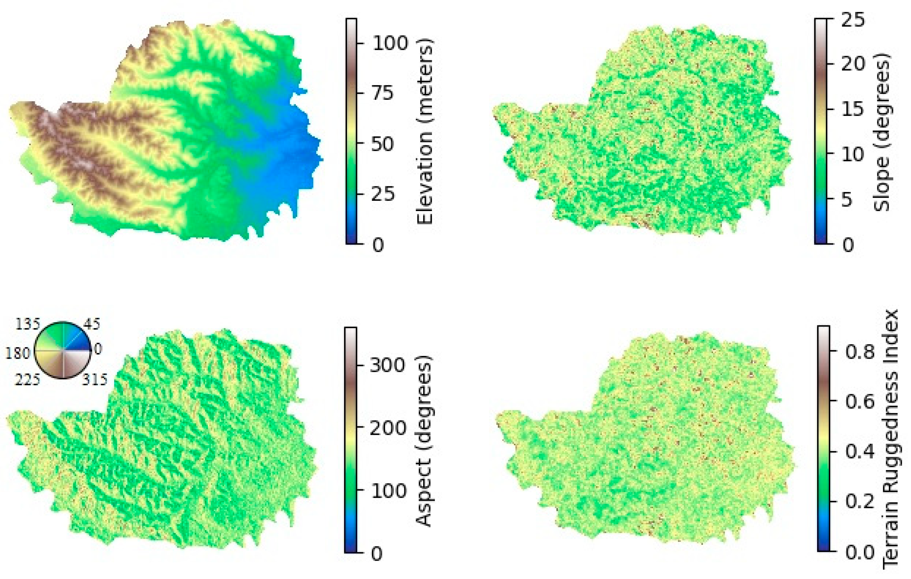
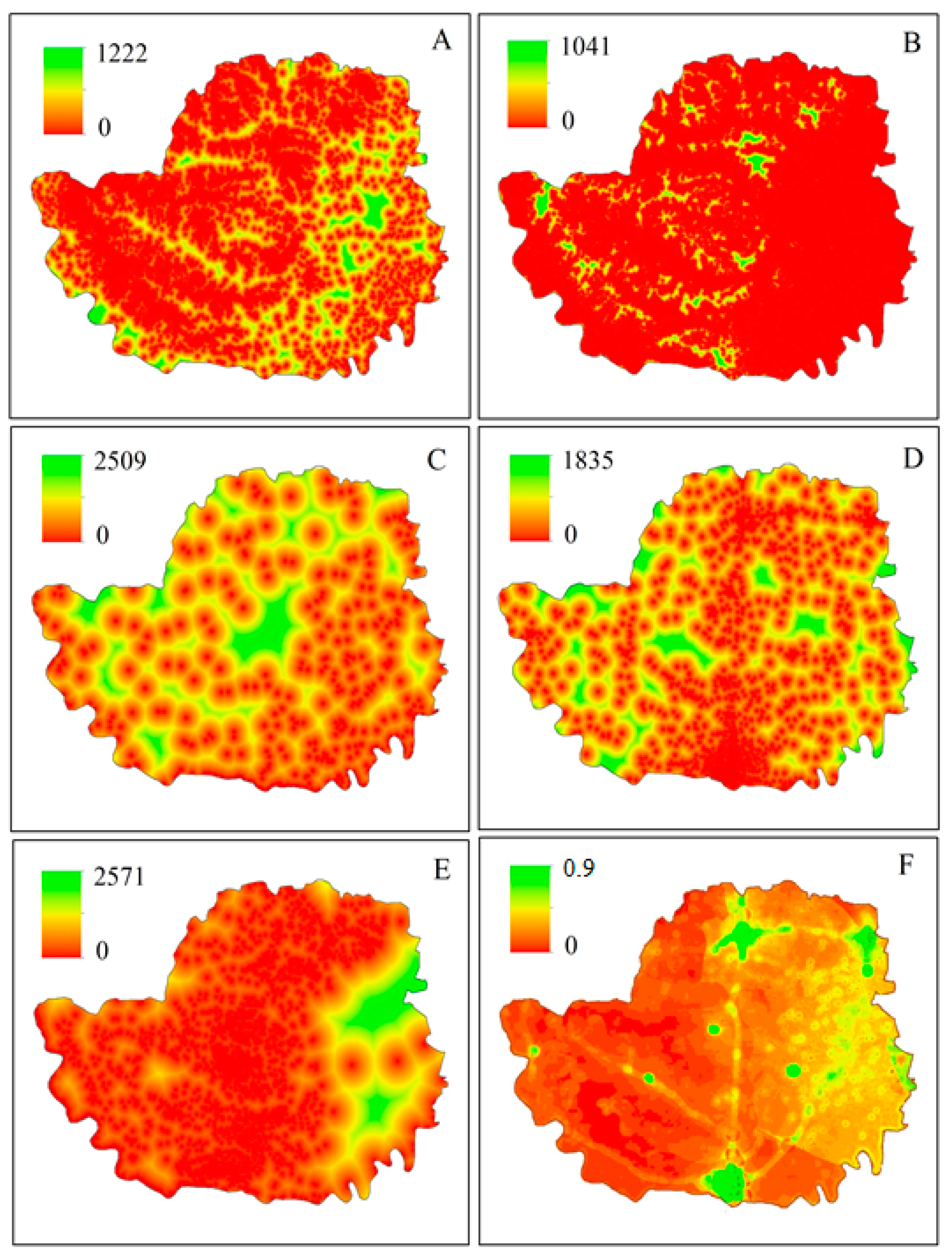
2.2.2. Satellite-Based Predictor Variables

Yearly mean composition was used for Landsat-5 and Landsat-8, because multi-image composition provides accurate predictions [34]. The used predictor variables for LULC classification are shown in Table 3. Along with spectral bands, various spectral indices: NDVI [35], NDBI [36], MNDWI [37], and BSI [38], were used for LULC classification. The topographic drivers (elevation, aspect, and slope) from DEM were included to distinguish water bodies from other LULC types [39,40]. Slope and aspect were computed using the “ee.Terrain” function in GEE. NTL data from DMSP-OLS and VIIRS were also used to distinguish the built-up areas from other LULC types [41,42].

2.2.3. LULC Categories and Reference Data

The LULC was classified into five categories: built-up land (BUL), forest land (FL), agricultural land (AL), water body (WB), and barren land (BL), from Google Earth images and field surveys (Table 4). Over 1200 reference points were visually marked for each year (2006, 2014, and 2021) from high-resolution (resolution < 2.5 m) Google Earth images. Sampling points were randomly collected from each LULC type, ensuring at least 50 points per category. A detailed ground survey was also conducted in 2021 and collected 247 sampling points, which were also used for both training and validating.

2.2.4. LULC Classification and Accuracy Assessment

The Random Forest (RF) model [43] was used for classification on the GEE platform. Recently, the RF model has gained attention for various ecological modeling tasks, such as biomass prediction [44], ecotope mapping [45], canopy cover prediction [46], soil organic carbon mapping and prediction [47], species distribution modeling [48], and land use land cover classification [49], due to its superior performance compared to other models [43]. In RF classification, two key tuning parameters are significant: ntree and mtry [50]. Mtry is the number of predictor variables selected at each node, and the default value (square root of the total predictors) provides better results [41]. The second tuning parameter is ntree, which controls the total number of independent trees. Having lots of trees is conducive to stabilizing the variable importance [50] and variable interaction [51]. Therefore, the default value of mtry and 1000 ntree were used for the LULC classification.
Sampling points of all three years were divided randomly into two sets: 70% of the data were allocated for training, and the remaining 30% was set aside for validation. We produced the confusion matrix of LULC to assess the accuracy using the producer’s accuracy, user’s accuracy, F1 score, overall accuracy, and Kappa’s coefficient [52,53].

2.3. LULC Prediction for the Year 2030 Using LCM

The Land Change Modeler (LCM) in TerrSet (version 19) is a LULC change detection and prediction tool developed by Clark Labs [54,55]. For future LULC prediction, the minimum requirements are (1) two land cover maps to understand the changes or transitions, and (2) driving factors to generate the transition-potential maps which indicate the suitability for transitions [56]. The details of the methodological design are shown in Figure 2. However, LCM combines three main steps: (1) change analysis; (2) transition potentials; and (3) change prediction.

2.3.1. Change Analysis

The change analysis in LCM provides the differences between LULC maps and identifies the transitions from one LULC class to another. The basic needs of the model are two periods of LULC maps, as well as an optional elevation layer and road layer, which were used as input. But it is also important to identify the dominant transitions between LULC classes, because dominant transitions only have significant impacts on altering the landscape dynamics of an area [56], and also reduce the computational burden [57]. Therefore, transitions below 500 ha were excluded to identify the dominant transitions in this study.

2.3.2. Transition Potentials

Transition potentials indicate the suitability for transitions between land classes. After identifying dominant transitions from change analysis, transitions were modeled using sub-models in the transition potentials module. This section facilitates users assigning the transitions that share common underlying drivers [58]. We assume that all transitions in our study area are affected by the same driver variables. Therefore, all transitions were grouped into a single model and named ‘disturbance’.
Land cover transitions are affected by several drivers [57]. Therefore, drivers are considered according to their availability and their impact on LULC changes. A total of ten factors, such as elevation, slope, Terrain Ruggedness Index (TRI), aspect, distance from built-up, distance from water body, distance from forest, distance from road, distance from agriculture land, distance from barren land, and population were considered as drivers for all transitions (Figure 3 and Figure 4). The vector road data (primary, secondary, and tertiary roads) were collected from OpenStreetMap. The distance from the road was computed using Euclidean distance in the spatial analyst tools of ArcGIS (version 10.4.1). SRTM-DEM elevation data were collected from GEE (see Section 2.2.1 “Satellite data”), and then slope, aspect, and TRI were computed in ArcGIS. Forest land, water bodies, built-up land, agricultural land, and barren land were derived from the LULC map, and the distance from built-up, forest land, agriculture land, water body, and barren land were computed using Euclidean distance in the spatial analyst tools of ArcGIS. The distance measurement indicates how far a particular point is from the nearest area of each specified land type. The World Pop population data (https://www.worldpop.org/, accessed on 22 August 2024) available in GEE were employed to extract the population. After that, Cramer’s V was calculated for these drivers. We selected variables having Cramer’s V ≥ 0.15 for the transition potential analysis, as they are generally considered useful [59].
After identifying the major transitions and useful drivers, the Multi-Layer Perceptron Neural Network (MLP-NN) was used to produce transition potential maps, as the MLP can run multiple transitions in a single sub-model [60]. MLP is efficient in computation, straightforward, and effective at modeling nonlinear relationships compared to other methods [60]. During training the MLP model, we used an automatic mode that operates without requiring user intervention [58]. We obtained transition potential maps with an overall accuracy of 82%, which mainly depended on the drivers used for modeling [61].

2.3.3. Change Prediction

The Markov chain model was used to generate transition probability for the future, indicating the land that is expected to change from the subsequent date to the anticipated date. This is based on converting one class to another by using the conditional probability between the earlier and later LULC maps [59]. A constraint layer was also added for areas that were not expected to change in the future. We used preserved parks, airports, and major buildings as administrative constraints, and major water bodies as natural constraints. We used a value of “0” for constrained areas and “1” for unconstrained areas, as recommended by TerrSet (Figure 5). After that, we ran the model and obtained both hard predictions and soft predictions. The hard prediction indicates land use class, whereas the soft prediction predicts values ranging from zero (indicating low susceptibility to change) to one (indicating high susceptibility), reflecting their susceptibility to the change.

2.3.4. Model Validation

Firstly, the LULC maps from 2006 and 2014, along with major drivers, were used as input for predicting the LULC of 2021. Then, the predicted LULC map of 2021 was compared with the classified LULC map of 2021, and no notable discrepancies were found (Table 5 and Figure 6). Also, Kappa statistics-related relevant statistics, such as Kappa Standard (Kstandard), Kappa No Information (Kno), and Kappa Location (Klocation), were computed to assess the agreement between the classified and predicted maps using the “validate” function in TerrSet. The Kno is the kappa for no additional information, Klocation is the kappa for grid-cell level location, and Kstandard is the standard Kappa index of agreement [62]. We obtained Kstandard = 0.818, Kno = 0.856, and Klocation = 0.841, indicating strong agreement between the predicted and classified maps and confirming the reliability of the model predictions [62]. After a successful prediction for 2021 with good agreement, we conducted change analysis, assessed transition potential, and generated transition probability for 2030, using the LULC maps from 2006 and 2021 to predict the LULC for 2030.

2.4. Estimation of Carbon Stock and Sequestration Using ESM

The Ecosystem Services Modeler (ESM) in TerrSet (version 19) is a spatial decision support tool for evaluating the worth of natural resources for promoting sustainable development. The Ecosystem Services Modeler provides various models that are closely aligned with the InVEST toolset (https://clarklabs.org/: accessed on 12 March 2023). The carbon storage and sequestration model in the ESM was employed to estimate carbon stock and sequestration. This model estimates the carbon stock in the landscape, as well as changes in carbon stock over time, along with economic valuation. However, the basic needs of this model are (1) LULC images, (2) carbon pools table, and optionally (3) the economic value of carbon.

2.4.1. LULC Images

LULC images of 2006, 2021, and 2030 were used as inputs for estimating carbon storage and sequestration. The LULC image of 2030 was used as a future LULC image, for estimating carbon stock and sequestration in the future.

2.4.2. Carbon Pools Table

The carbon pools table of each LULC type was generated from the field survey, laboratory analysis, and literature review. For carbon stock and sequestration modeling using the Ecosystem Service Modeler (ESM), it is essential to have data on the carbon stocks in these carbon pools: above ground (C above), below ground (C below), dead organic matter (C dead), and soil carbon (C soil) (Table 6). Carbon stocks in four carbon pools in forest land (FL) were estimated through field surveys and laboratory analysis (Supplementary Materials), and the average carbon stock of each pool was used for this study (Table S1). Deadwood and litter carbon stocks of forest land were lumped together as dead organic matter (C dead) of forest land, as recommended by IPCC 2006 [63]. Soil organic carbon (SOC or C soil) of agricultural land, barren land, and built-up land was estimated using the method used for SOC estimation in forests (for details see Section S3 “Carbon stored in soil” in Supplementary Materials).
A minimum of 10 soil samples were randomly collected from each LULC type, and the mean carbon stock of each LULC type was used for this study. The SOC stocks of each LULC type were estimated through field surveys and laboratory analyses, because (1) SOC stock in the surface layer varies widely among different forest types and climate regions across the world [63], and (2) SOC data at a depth of 0–10 cm for this forest type and climatic region was not available in the literature and reports. Carbon stocks of remaining carbon pools of LULC types were generated using reports and literature review [4,63].

2.4.3. Economic Valuation

The value of carbon was added as a social value of USD 185 per ton of CO2 at a 2% market discount rate [64], and it was assumed that the price of carbon would remain constant. The economic value of carbon sequestration was measured using net present value (NPV). The NPV of carbon sequestration was measured using the following equation:
N P V = C a × P c / ( 1 + i ) t
NPV is the net present value, C a is the carbon stock (Mg), P c is the price of carbon per Mg, i is the discount rate, and t is the time period.

3. Results

3.1. LULC Types and Accuracy

The area of LULC types and the accuracy of classification are shown in Table 7. Our LULC classifications demonstrated strong performance, with overall accuracy (OA) and Kappa’s coefficient (K) scores of 0.900 and 0.857 for 2006, 0.937 and 0.911 for 2014, and 0.894 and 0.850 for 2021, respectively. For all of the classified years, agricultural land was the largest distributed LULC, followed by forest land, barren land, built-up land, and water bodies (Table 7 and Figure 7).

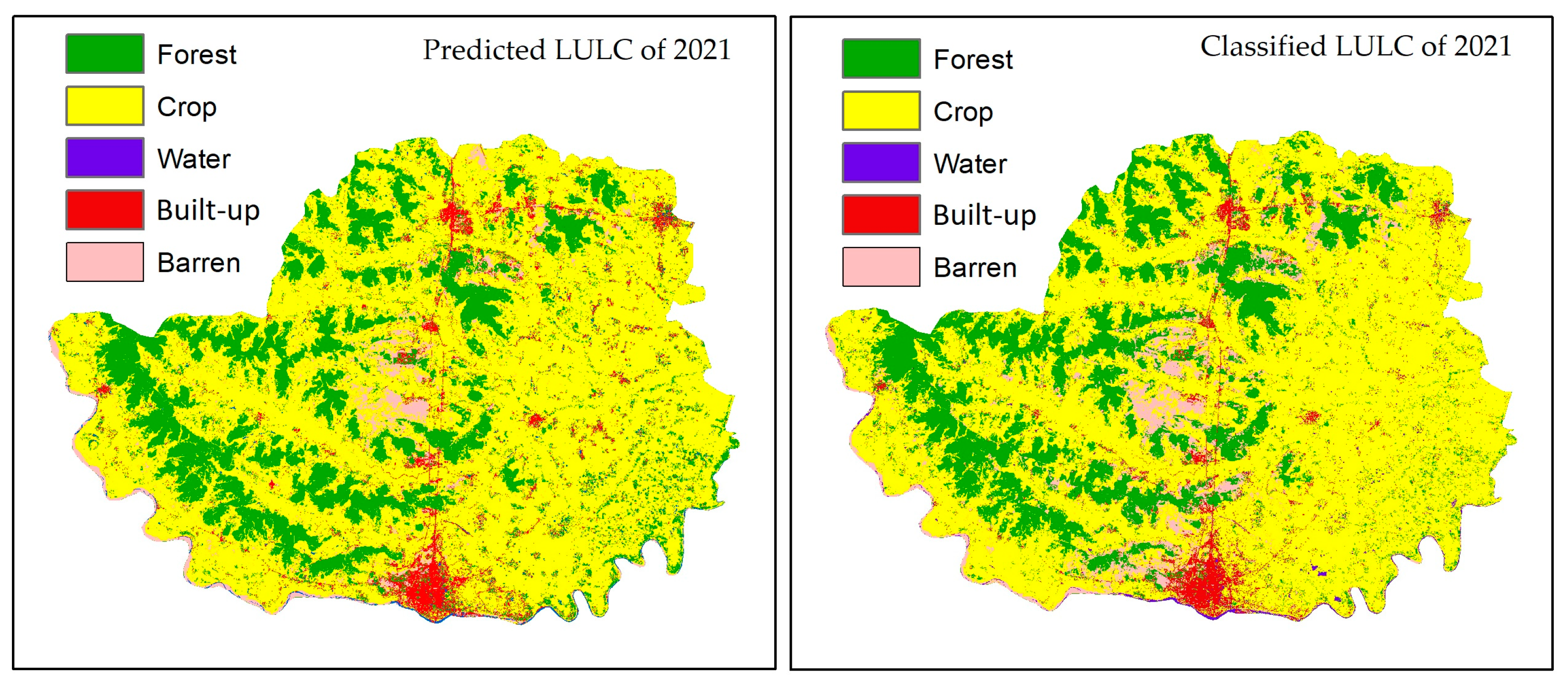
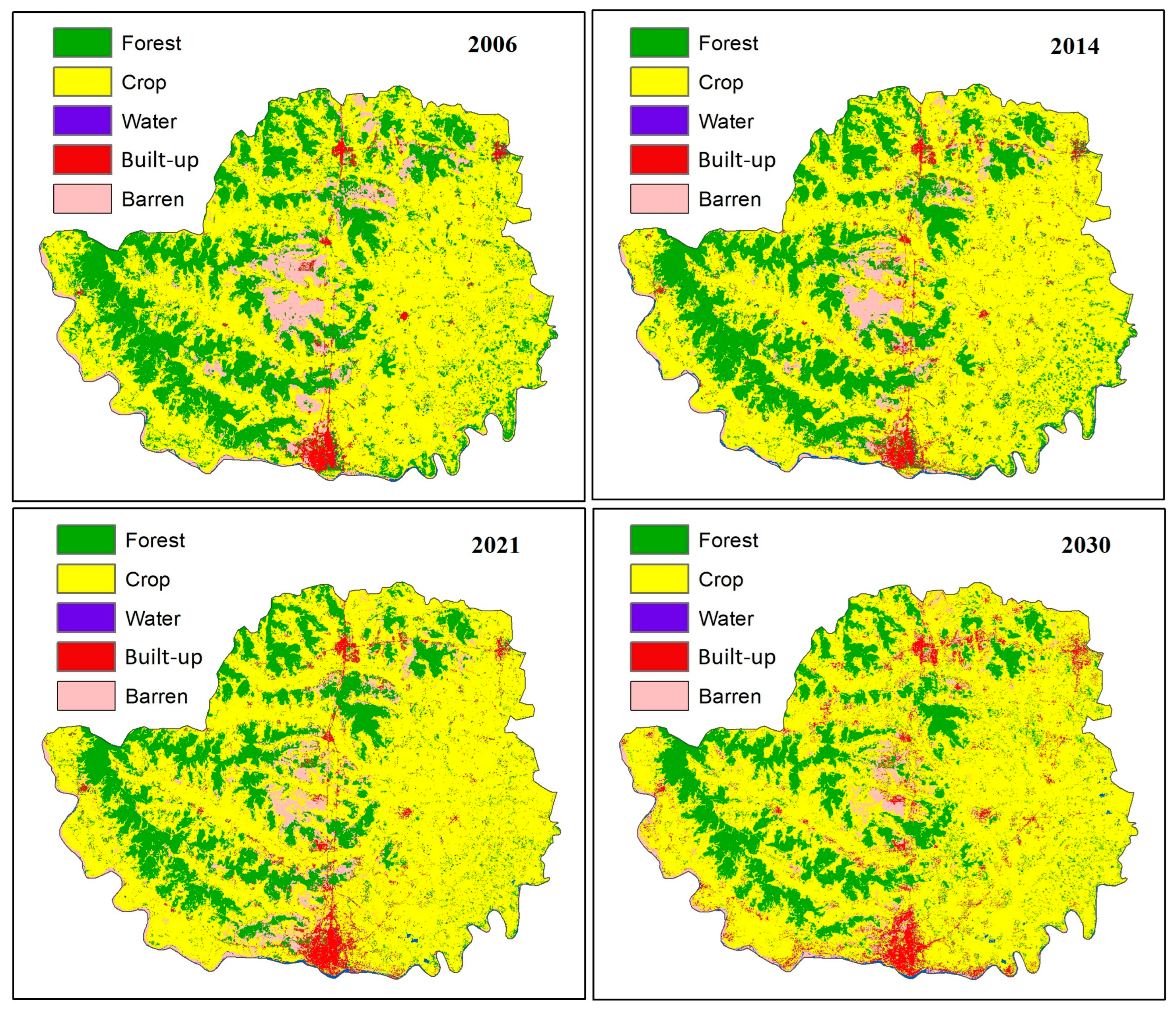
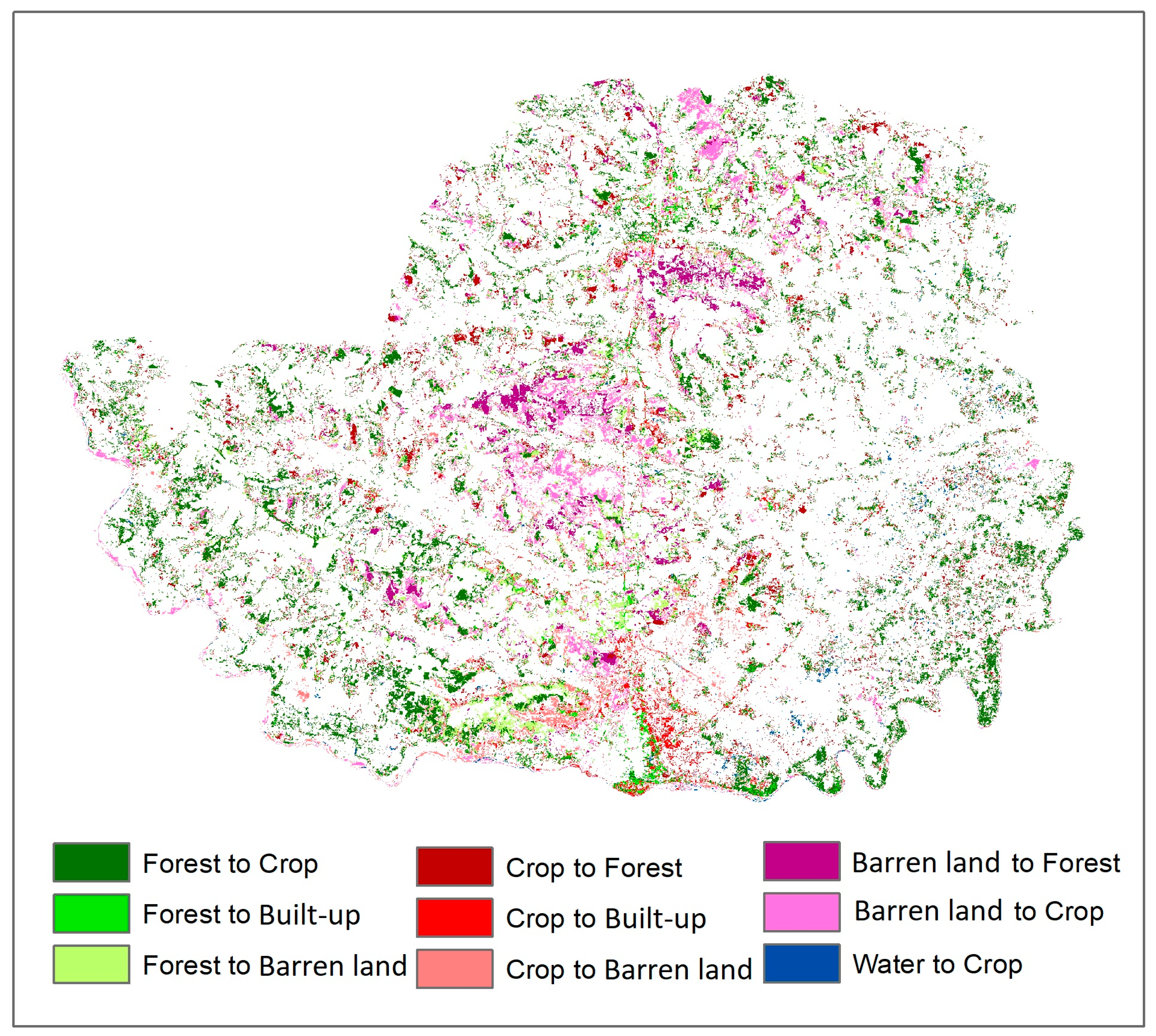
3.2. LULC Change and Prediction

LULC changes from 2006 to 2021 are shown in Table 8. As we ignored the transitions below 500 ha for the prediction model, we identified nine dominant transitions or changes from 2006 to 2021 (Figure 8). Between 2006 and 2021, the forest area diminished by −108.606 sq. km (Table 9) and dominantly changed into agricultural land (136.068 sq. km), then into barren land (24.490 sq. km) and built-up land (13.293 sq. km). Water bodies and barren land also decreased by −2.478 sq. km and −19.401 sq. km, respectively (Table 9). Barren lands were dominantly changed into agricultural (41.597 sq. km) and forest land (26.171 sq. km), while water bodies were dominantly changed into agricultural land (7.083 sq. km). There was also an increase in agricultural land of 98.624 sq. km and in built-up land of 31.862 sq. km. The increase in agricultural land from 2006 to 2021 was mainly driven by significant reductions in forest land, barren land, and water bodies (Table 8). However, the increase in built-up land was mostly derived from agricultural land and forest land. Despite agricultural land being dominantly converted into forest, barren, and built-up land, net positive growth was observed for agricultural land due to a large amount of forest land (136.068 sq. km) being converted into agricultural land (Table 8). So, net negative growth was also observed for forest land, despite the conversion of barren land and agricultural land into forest land (Table 8). However, the two most dominant changes observed were as follows: (1) net positive growth for agriculture; (2) net negative growth for forests because a substantial portion of forest land was converted into agricultural land.
Transition probability for the year 2030 on the basis of changes from 2006 to 2021 is shown in Table 10, which indicates the likelihood of a class transitioning into other classes in the upcoming predicted year. There is a 0.742 probability that forest land will remain as forest land for 2030, and the highest probability is 0.195 that forest land will convert into agricultural land, then into barren land (probability: 0.042) and built-up land (probability: 0.020). For agriculture land, there is a 0.941 probability that agricultural land will remain in the same class, which is the highest probability among the LULC types. The highest probability is 0.023 that agricultural land will convert into forest land, then into barren land (probability: 0.019) and built-up land (probability: 0.014). There is only a 0.553 probability that barren land will remain as barren land for 2030, indicating that barren land is more likely to convert to other land (probability: 0.447), and has the highest likelihood of being converted into agricultural land and forest land (Table 10). After barren land, there is only a 0.578 probability that the water body will remain as the water body, and it is more likely (probability: 0.306) to be converted into agricultural land.
The LCM-based, predicted LULC map is shown in Figure 7. The LCM predicted that agricultural land and built-up land will increase, while barren land, forest land, and water bodies will decrease by the year 2030 (Table 9). It was projected that the highest percentage of growth would be observed in built-up land, which is expected to increase by approximately 33% (21.761 sq. km) from 66.470 sq. km in 2021 to 88.231 sq. km in 2030. Conversely, it was also observed that barren land is going to reduce by approximately 24% from 2021 to 2030 (Table 9).

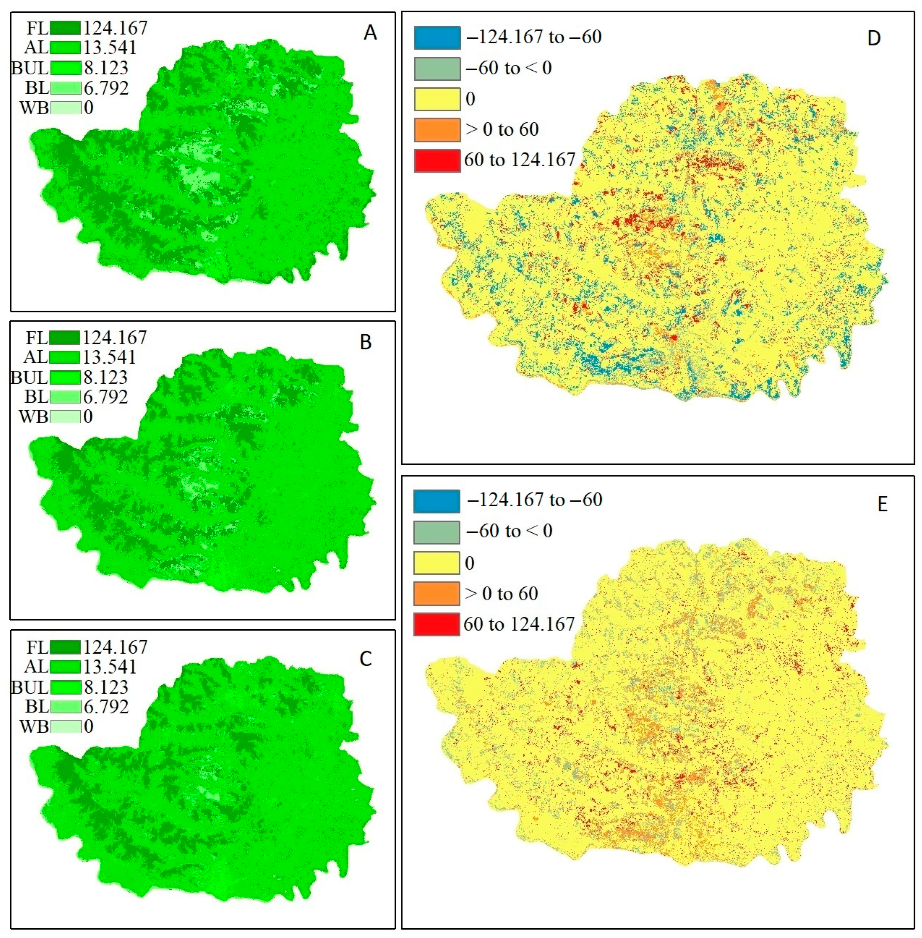
3.3. Carbon Stock and Sequestration with Economic Valuation

Total carbon stock in the study regions was 78.853 Tg in 2006, comprising carbon present in forest land (62.349 Tg), agricultural land (15.293 Tg), barren land (0.931 Tg), and built-up land (0.281 Tg) (Table 11). The highest carbon was stored in forest land (124.167 Mg/ha), and carbon storage outside the forest declined to 13.541 Mg/ha for agricultural land and 0–8.123 Mg/ha for the water bodies, built-up land, and barren land (Figure 9).
The study area had a total carbon stock of 66.843 Tg in 2021, representing a decrease (release into the atmosphere) of 12.010 Tg compared to the total carbon stock in 2006 (Table 11). Although the carbon stock per unit area remains consistent with that of 2006, carbon stock in each LULC type has changed due to LULC alterations from 2006 to 2021. The changes in carbon stock between 2006 and 2021 are shown in Figure 9. Carbon stock decreased by 13.471 Tg in forest land and 0.133 Tg in barren land as both forest land and barren land decreased from 2006 to 2021. Conversely, there was an increase in carbon stock (sequestration) in agricultural and built-up areas by 1.336 Tg and 0.259 Tg, respectively. But a large amount of carbon was lost from forest land (13.471 Tg: nearly 99% of the total carbon loss), which played an active role in the reduction in the total carbon stock in 2021.
Predicted carbon stock for 2030 and changes from 2021 to 2030 are shown in Figure 9 and Table 11. The total stock as per the prediction for 2030 is 64.308 Tg, which indicates a likelihood of a further decrease by 2.536 Tg compared to the total carbon stock in 2021. From 2021 to 2030, carbon stock is likely to increase in agricultural land (0.418 Tg) and built-up land (0.177 Tg). But carbon stock is likely to decrease by 2.943 Tg in forest land and 0.186 Tg in barren land from 2021 to 2030, as forest land and barren land are likely to further decrease during this period (Table 9). However, as a large amount of loss is likely to be caused by forest land (2.943 Tg: nearly 94% of the total carbon loss), the total stock is likely to decline in 2030 compared to 2021.
Due to the continuous decrease in carbon stock, the economic value of carbon stock has continuously decreased from 2006 (USD 1458.787 million) to 2021 (USD 1236.604 million), and is likely to decrease further by the year 2030 (USD 1193.210 million) (Table 12). From 2006 to 2021, the economic value of carbon sequestration decreased by USD 222.183 million, with an average annual change rate of USD 14.812 million. However, the present value of carbon stock is USD 1236.604 million in the year 2021, and it is expected to decline by USD 43.394 million by the year 2030, with an average annual net present value (NPV) of sequestration USD -4.822 million (Table 12).

4. Discussions

In this study, carbon stock and sequestration, and their economic values, were assessed due to LULC changes. The economic value is proportional to carbon stock in a landscape, is generally calculated to increase awareness among the people and to help in understanding the significance of a particular ecosystem service in terms of monetary value [4]. Based on the results, it is evident that total carbon stock and economic value decreased from 2006 to 2021 and are expected to decrease further by the year 2030. Forest land alone contributed 99% of the carbon loss and is likely to contribute 94% in the future due to the conversion of forest land into other LULC types, primarily into agricultural land. The reduction of carbon stock, mainly due to forest loss, is quite consistent with the findings of [24], who found that natural forest cover loss has been increasing in these areas as a result of anthropogenic activities. Carbon storage in forest land was almost 124.167 Mg/ha, and carbon storage outside the forest declined to 13.541 Mg/ha for agricultural land and 0–8.123 Mg/ha for the water bodies, built-up land, and barren land. Forest land occupied 21.529% of the study area in 2021, and was storing almost 73.122% of the carbon stock. This indicates the significance of forests in carbon stock and sequestration. Therefore, reducing deforestation and increasing regeneration/afforestation should be the primary approach for reducing carbon emissions from the forests and increasing sequestration from the atmosphere [65]. Barren land occupied 6.415% of the total study area and stored only 1.193% of total carbon stock in 2021. Plantations in barren lands would be a better option for increasing forest cover and carbon stock. Plantations should be introduced in regions that experienced carbon loss between 2006 and 2021 due to LULC changes (Figure 9). As various previous studies found, tree diversity has positive effects on carbon stock [66]. Therefore, planting a variety of tree species would be more advantageous for enhancing carbon stock while maintaining biodiversity and ecosystem services, as a single tree species cannot provide the optimum level of biodiversity and ecosystem services [24].
The annual overall carbon stock reduction rate is projected to decline slightly in the future (annual loss expected: 0.282 Tg) compared to loss during 2006–2021 (annual loss: 0.801 Tg). The reasons for decline are (1) barren land is expected to decline by approximately 24% from 2021 to 2030, and it has the highest likelihood of being converted into forest land and agricultural land, which have a higher carbon stock per unit area than barren land; (2) although overall agricultural land is expected to increase, agricultural land is also expected to undergo conversion into forests; and (3) forest loss is expected to decline during 2021–2030 compared to the loss observed between 2006 and 2021 (Table 9). Our study found that 26% (probability 0.7422 that forests will remain as forests) of forest land is expected to convert into other lands (Table 10), but overall forest cover is expected to decline only by 5.764% (23.567 sq. km), which means other LULC types are likely to convert into forests. The authors of [24] reported an increase in natural forest loss and at the same time an increase in the plantations of monoculture exotic species in these regions. Due to the increase in plantations, along with deforestation, the percentage of forest cover is not changing significantly. But, the fact is that the loss of mature natural forests or their conversion to other LULC types is leading to significant carbon emissions into the atmosphere. Therefore, it is crucial to control natural forest cover loss, as mature natural forests store more carbon stock than newly planted forests [67,68]. This is because carbon stock positively depends on age and productivity [69,70]. Also, we found that overall carbon stock is expected to decline, mainly due to the conversion of forest land into agricultural land. Built-up areas are expected to increase due to the reduction in agricultural and forest lands. Consequently, the growth of built-up areas is leading to a reduction in carbon stock, as built-up areas have lower carbon stocks per unit area compared to forest and agricultural lands.
Previous studies found that the main reasons for natural forest cover loss are logging and agricultural expansion due to demographic growth in this region [24]. Demographic growth accelerates urbanization and agricultural activity for economic development [71]. Therefore, reducing deforestation from residential urban growth and agricultural activity should be the main strategy for controlling deforestation. Urgent protection measures should be implemented in areas where forest cover loss and carbon loss are expected in the future (Figure 9). Although the Government of India has enacted several forest-related policies over time (such as the Indian Forest Act of 1927, the Wildlife Protection Act of 1972, the Forest Conservation Act of 1980, the Biological Diversity Act of 2002, and the Scheduled Tribes and Other Traditional Forest Dwellers Act of 2006), land use and land cover (LULC) transitions and deforestation still remain primary issues for local communities [24]. This suggests that there is insufficient strengthening of forest-related policies at the regional level and an inability to address the critical needs of local communities. So, secure tenure rights, proper management practices, and proper implementation of relevant laws and policies can be crucial for effective forest management and increasing carbon stock. Various studies have reported that secure tenure rights motivate individuals to take part in reforestation and afforestation activities [72,73], and play a crucial role in forest protection [74,75]. As most of the people in these regions depend on forests and a variety of factors contribute to forest loss [24], community-based management strategies [76] could be effective for increasing carbon stock through expansion of forest cover, benefitting local communities [77]. The Joint Forest Management (JFM) policy plays a significant role for protecting forests, promoting afforestation, and providing economic benefits to rural communities [78,79]. A robust implementation of the JFM policy in these areas has the potential to foster favorable social interactions, promote afforestation and conservation practice, and generate economic benefits for the local community. Also, agroforestry can be effective, instead of just agriculture, to enhance biodiversity and ecosystem services [80,81,82].
However, the current study examines the impacts of LULC types on carbon stocks and sequestrations, and depicts the importance of LCM and ESM for measuring carbon stock and sequestration in relation to the LULC types, but there are a few limitations for this study. Ecosystem Services Modeler (ESM) assumes change occurs linearly over time, and it does not have the option to add biophysical conditions, such as photosynthesis rates, nutrient availability, activities of soil microorganisms, and soil types, which has effects on carbon sequestration [4]. Inclusion of wood harvest rates, and harvested product degradation rates can help improve the accuracy of the estimation of carbon stock and sequestration. Also, the inclusion of other socioeconomic drivers and government management policies, and climatic variables of LULC changes can improve LULC prediction as well as future carbon stock prediction. For this study, LULC was classified into five categories at 30 m resolution. Increasing the number of LULC classes using higher resolution satellite images could potentially lead to more precise and efficient results. Furthermore, some values for carbon stock density are based on default values obtained from reports and literature reviews rather than field study. Therefore, future research should be focused on and tested using the above parameters to address these limitations.

5. Conclusions

This work examined the carbon stocks and sequestrations in relation to the LULC changes in present and future scenarios using the integration of LCM and ESM in the tropical dry deciduous forests of West Bengal, India. The results indicate that total carbon stock and its economic value decreased during the period from 2006 to 2021 and are expected to decline further by 2030 due to the conversion of forest lands primarily into agricultural land. The dynamic nature of forests and the loss of mature forests due to demographic growth are significantly affecting carbon stocks. Therefore, this study suggests that multi-species plantations, secure tenure rights, proper management practices, and better implementation of forest-related policies can increase carbon stock and sequestration. Although there are a few limitations in this study, this study provides a detailed understanding of the spatial and temporal dynamics of carbon stock and sequestration in different LULC types. These types of spatial–temporal information can be helpful for mitigation strategies by providing guidelines to the policymakers. Also, the integration of LCM and ESM in TerrSet provides a robust setup for analyzing the LULC changes and their effects on ecosystem services, which can be applied in broader contexts in different geographical areas.

Supplementary Materials

The following supporting information (which includes [83,84,85,86,87,88,89,90,91,92,93,94,95,96,97,98,99,100,101,102]) can be downloaded at: https://www.mdpi.com/article/10.3390/land13101689/s1, Table S1: Carbon stock in the different carbon pools of dry deciduous forests. The numbers before and after the “±” symbol indicate average and standard error, respectively. The highlighted numbers were used in the Carbon pools table for assessing carbon stock and sequestration. Figure S1: Nested square-shaped sample plot for field surveys. 30 m × 30 m plot used for measuring trees with diameter at breast height (DBH) greater than 30cm, dead woods, and climbers; 15 m × 15 m plot used for measuring trees with diameter at breast height (DBH) 10-30 cm; 7.5 m × 7.5 m plot used for measuring trees with diameter at breast height (DBH) 5-10 cm; 3 m × 3 m plots used for measuring juveniles and shrubs; 1 m × 1 m plots used for measuring seedlings, herbs, grasses, and litter; The letter ‘S’ represents the location of soil samples.

Author Contributions

Conceptualization, D.B. and M.Z.; methodology, D.B. and S.G.; software, D.B. and S.G.; validation, D.B. and S.G.; formal analysis, D.B. and S.D.; investigation, N.D.C., D.B. and M.Z.; resources, D.B. and N.D.C.; data curation, D.B.; writing—original draft preparation, D.B.; writing—review and editing, N.D.C., S.D., V.D., S.G., B.C., B.B. and M.Z.; visualization, D.B., V.D., N.D.C. and S.D.; supervision, N.D.C.; funding acquisition, D.B.; project administration, D.B. and M.Z. All authors have read and agreed to the published version of the manuscript.

Funding

This research was supported by the Researchers Supporting Project (Grant number RSP2024R296), King Saud University, Riyadh, Saudi Arabia. This research was funded by the Council of Scientific and Industrial Research (CSIR), Government of India, in the form of Senior Research Fellowship, grant number (09/599/(0083)/2019-EMR-I).

Data Availability Statement

The original contributions presented in the study are included in the article/Supplementary Materials; further inquiries can be directed to the corresponding author.

Acknowledgments

We would like to express our sincere gratitude to the Council of Scientific and Industrial Research (CSIR), Government of India, for their financial support. We also extend our heartfelt thanks to all our colleagues in the lab for their continuous help, support, and encouragement throughout this research.

Conflicts of Interest

The authors declare no conflicts of interest.

References

  1. Ravindranath, N.H.; Ostwald, M. Carbon Inventory Methods: Handbook for Greenhouse Gas Inventory, Carbon Mitigation and Roundwood Production Projects; Springer: Dordrecht, The Netherlands, 2008; ISBN 978-1-4020-6546-0. [Google Scholar]
  2. IPCC. Climate Change 2021: The Physical Science Basis. Contribution of Working Group I to the Sixth Assessment Report of the Intergovernmental Panel on Climate Change; Masson-Delmotte, V., Zhai, P., Pirani, A., Connors, S.L., Péan, C., Berger, S., Caud, N., Chen, Y., Goldfarb, L., Gomis, M.I., et al., Eds.; Cambridge University Press: Cambridge, UK, 2021. [Google Scholar]
  3. IPCC. Climate Change 2007: The Physical Science Basis. Contribution of Working Group I to the Fourth Assessment Report of the Intergovernmental Panel on Climate Change; Solomon, S., Qin, D., Manning, M., Chen, Z., Marquis, M., Averyt, K.B., Tignor, M., Miller, H.L., Eds.; Cambridge University Press: Cambridge, UK, 2007. [Google Scholar]
  4. Babbar, D.; Areendran, G.; Sahana, M.; Sarma, K.; Raj, K.; Sivadas, A. Assessment and Prediction of Carbon Sequestration Using Markov Chain and InVEST Model in Sariska Tiger Reserve, India. J. Clean. Prod. 2021, 278, 123333. [Google Scholar] [CrossRef]
  5. Zhang, J.; Ge, Y.; Chang, J.; Jiang, B.; Jiang, H.; Peng, C.; Zhu, J.; Yuan, W.; Qi, L.; Yu, S. Carbon Storage by Ecological Service Forests in Zhejiang Province, Subtropical China. For. Ecol. Manag. 2007, 245, 64–75. [Google Scholar] [CrossRef]
  6. Zhang, F.; Zhan, J.; Zhang, Q.; Yao, L.; Liu, W. Impacts of Land Use/Cover Change on Terrestrial Carbon Stocks in Uganda. Phys. Chem. Earth Parts A/B/C 2017, 101, 195–203. [Google Scholar] [CrossRef]
  7. García, M.; Riaño, D.; Chuvieco, E.; Danson, F.M. Estimating Biomass Carbon Stocks for a Mediterranean Forest in Central Spain Using LiDAR Height and Intensity Data. Remote Sens. Environ. 2010, 114, 816–830. [Google Scholar] [CrossRef]
  8. Dixon, R.K.; Solomon, A.M.; Brown, S.; Houghton, R.A.; Trexier, M.C.; Wisniewski, J. Carbon Pools and Flux of Global Forest Ecosystems. Science 1994, 263, 185–190. [Google Scholar] [CrossRef]
  9. Agboola, O.O.; Mayowa, F.; Adeonipekun, P.A.; Akintuyi, A.; Gbenga, O.; Ogundipe, O.T.; Omojola, A.; Alabi, S. A Rapid Exploratory Assessment of Vegetation Structure and Carbon Pools of the Remaining Tropical Lowland Forests of Southwestern Nigeria. Trees For. People 2021, 6, 100158. [Google Scholar] [CrossRef]
  10. Behera, S.K.; Sahu, N.; Mishra, A.K.; Bargali, S.S.; Behera, M.D.; Tuli, R. Aboveground Biomass and Carbon Stock Assessment in Indian Tropical Deciduous Forest and Relationship with Stand Structural Attributes. Ecol. Eng. 2017, 99, 513–524. [Google Scholar] [CrossRef]
  11. Xu, L.; Saatchi, S.S.; Shapiro, A.; Meyer, V.; Ferraz, A.; Yang, Y.; Bastin, J.-F.; Banks, N.; Boeckx, P.; Verbeeck, H.; et al. Spatial Distribution of Carbon Stored in Forests of the Democratic Republic of Congo. Sci. Rep. 2017, 7, 15030. [Google Scholar] [CrossRef]
  12. Chazdon, R.L.; Broadbent, E.N.; Rozendaal, D.M.A.; Bongers, F.; Zambrano, A.M.A.; Aide, T.M.; Balvanera, P.; Becknell, J.M.; Boukili, V.; Brancalion, P.H.S.; et al. Carbon Sequestration Potential of Second-Growth Forest Regeneration in the Latin American Tropics. Sci. Adv. 2016, 2, e1501639. [Google Scholar] [CrossRef]
  13. Meister, K.; Ashton, M.S.; Craven, D.; Griscom, H. Carbon Dynamics of Tropical Forests. In Managing Forest Carbon in a Changing Climate; Ashton, M.S., Tyrrell, M.L., Spalding, D., Gentry, B., Eds.; Springer: Dordrecht, The Netherlands, 2012; pp. 51–75. ISBN 978-94-007-2232-3. [Google Scholar]
  14. Gaston, G.; Brown, S.; Lorenzini, M.; Singh, K.D. State and Change in Carbon Pools in the Forests of Tropical Africa. Glob. Change Biol. 1998, 4, 97–114. [Google Scholar] [CrossRef]
  15. Hosonuma, N.; Herold, M.; De Sy, V.; De Fries, R.S.; Brockhaus, M.; Verchot, L.; Angelsen, A.; Romijn, E. An Assessment of Deforestation and Forest Degradation Drivers in Developing Countries. Environ. Res. Lett. 2012, 7, 044009. [Google Scholar] [CrossRef]
  16. Houghton, R.A. Carbon Emissions and the Drivers of Deforestation and Forest Degradation in the Tropics. Curr. Opin. Environ. Sustain. 2012, 4, 597–603. [Google Scholar] [CrossRef]
  17. Kanninen, M. (Ed.) Do Trees Grow on Money? The Implications of Deforestation Research for Policies to Promote REDD; Forest perspectives; Center for International Forestry Research: Situ Gede, Bogor, Indonesia, 2007; ISBN 978-979-1412-42-1. [Google Scholar]
  18. Geist, H.J.; Lambin, E.F. Proximate Causes and Underlying Driving Forces of Tropical Deforestation. BioScience 2002, 52, 143. [Google Scholar] [CrossRef]
  19. Liu, Q.; Yang, D.; Cao, L.; Anderson, B. Assessment and Prediction of Carbon Storage Based on Land Use/Land Cover Dynamics in the Tropics: A Case Study of Hainan Island, China. Land 2022, 11, 244. [Google Scholar] [CrossRef]
  20. Liang, Y.; Hashimoto, S.; Liu, L. Integrated Assessment of Land-Use/Land-Cover Dynamics on Carbon Storage Services in the Loess Plateau of China from 1995 to 2050. Ecol. Indic. 2021, 120, 106939. [Google Scholar] [CrossRef]
  21. Gratani, L.; Varone, L.; Bonito, A. Carbon Sequestration of Four Urban Parks in Rome. Urban For. Urban Green. 2016, 19, 184–193. [Google Scholar] [CrossRef]
  22. Areendran, G.; Sahana, M.; Raj, K.; Kumar, R.; Sivadas, A.; Kumar, A.; Deb, S.; Gupta, V.D. A Systematic Review on High Conservation Value Assessment (HCVs): Challenges and Framework for Future Research on Conservation Strategy. Sci. Total Environ. 2020, 709, 135425. [Google Scholar] [CrossRef]
  23. Dinda, S.; Ghosh, S.; Chatterjee, N.D. Understanding the Commercialization Patterns of Non-Timber Forest Products and Their Contribution to the Enhancement of Tribal Livelihoods: An Empirical Study from Paschim Medinipur District, India. Small-Scale For. 2020, 19, 371–397. [Google Scholar] [CrossRef]
  24. Bera, D.; Chatterjee, N.D.; Ghosh, S.; Dinda, S.; Bera, S.; Mandal, M. Assessment of Forest Cover Loss and Impacts on Ecosystem Services: Coupling of Remote Sensing Data and Public’s Perception in the Dry Deciduous Forest of West Bengal, India. J. Clean. Prod. 2022, 356, 131763. [Google Scholar] [CrossRef]
  25. Bera, D.; Das Chatterjee, N.; Bera, S.; Rana, A.; Paul, B. Determining Recent Trends of Forest Loss and Its Associated Drivers for Sustainable Management in the Dry Deciduous Forest of West Bengal, India. In Environmental Management and Sustainability in India: Case Studies from West Bengal; Sahu, A.S., Das Chatterjee, N., Eds.; Springer International Publishing: Cham, Switzerland, 2023; pp. 171–186. ISBN 978-3-031-31399-8. [Google Scholar]
  26. Bera, D.; Das Chatterjee, N.; Bera, S.; Ghosh, S.; Dinda, S. Comparative Performance of Sentinel-2 MSI and Landsat-8 OLI Data in Canopy Cover Prediction Using Random Forest Model: Comparing Model Performance and Tuning Parameters. Adv. Space Res. 2023, 71, 4691–4709. [Google Scholar] [CrossRef]
  27. West Bengal Forest Department, Government of West Bengal, India. Annual Administrative Report 2021–2022; West Bengal Forest Department, Government of West Bengal: Kolkata, India, 2022.
  28. NASA JPL NASA Shuttle Radar Topography Mission Global 1 Arc Second 2013. Available online: https://lpdaac.usgs.gov/products/srtmgl1v003/ (accessed on 21 March 2023).
  29. Farr, T.G.; Rosen, P.A.; Caro, E.; Crippen, R.; Duren, R.; Hensley, S.; Kobrick, M.; Paller, M.; Rodriguez, E.; Roth, L.; et al. The Shuttle Radar Topography Mission. Rev. Geophys. 2007, 45, RG2004. [Google Scholar] [CrossRef]
  30. Baugh, K.; Elvidge, C.D.; Ghosh, T.; Ziskin, D. Development of a 2009 Stable Lights Product Using DMSP-OLS Data. Proc. Asia-Pac. Adv. Netw. 2010, 30, 114. [Google Scholar] [CrossRef]
  31. Elvidge, C.D.; Ziskin, D.; Baugh, K.E.; Tuttle, B.T.; Ghosh, T.; Pack, D.W.; Erwin, E.H.; Zhizhin, M. A Fifteen Year Record of Global Natural Gas Flaring Derived from Satellite Data. Energies 2009, 2, 595–622. [Google Scholar] [CrossRef]
  32. Elvidge, C.D.; Baugh, K.; Zhizhin, M.; Hsu, F.C.; Ghosh, T. VIIRS Night-Time Lights. Int. J. Remote Sens. 2017, 38, 5860–5879. [Google Scholar] [CrossRef]
  33. Gorelick, N.; Hancher, M.; Dixon, M.; Ilyushchenko, S.; Thau, D.; Moore, R. Google Earth Engine: Planetary-Scale Geospatial Analysis for Everyone. Remote Sens. Environ. 2017, 202, 18–27. [Google Scholar] [CrossRef]
  34. Urbazaev, M. Assessment of the Mapping of Fractional Woody Cover in Southern African Savannas Using Multi-Temporal and Polarimetric ALOS PALSAR L-Band Images. Remote Sens. Environ. 2015, 166, 138–153. [Google Scholar] [CrossRef]
  35. Rouse, J.W.; Haas, R.H.; Schell, J.A.; Deering, D.W.; Harlan, J.C. Monitoring the Vernal Advancement and Retrogradation (Green Wave Effect) of Natural Vegetation. In NASA/GSFC Type III Final Report; NASA/GSFC: Greenbelt, MD, USA, 1974; Volume 371. [Google Scholar]
  36. Zha, Y.; Gao, J.; Ni, S. Use of Normalized Difference Built-up Index in Automatically Mapping Urban Areas from TM Imagery. Int. J. Remote Sens. 2003, 24, 583–594. [Google Scholar] [CrossRef]
  37. Xu, H. Modification of Normalised Difference Water Index (NDWI) to Enhance Open Water Features in Remotely Sensed Imagery. Int. J. Remote Sens. 2006, 27, 3025–3033. [Google Scholar] [CrossRef]
  38. Rikimaru, A.; Roy, P.S.; Miyatake, S. Tropical Forest Cover Density Mapping. Trop. Ecol. 2002, 43, 39–47. [Google Scholar]
  39. Margono, B.A.; Bwangoy, J.-R.B.; Potapov, P.V.; Hansen, M.C. Mapping Wetlands in Indonesia Using Landsat and PALSAR Data-Sets and Derived Topographical Indices. Geo-Spat. Inf. Sci. 2014, 17, 60–71. [Google Scholar] [CrossRef]
  40. Jones, J.W. Efficient Wetland Surface Water Detection and Monitoring via Landsat: Comparison with in Situ Data from the Everglades Depth Estimation Network. Remote Sens. 2015, 7, 12503–12538. [Google Scholar] [CrossRef]
  41. Shi, K.; Huang, C.; Yu, B.; Yin, B.; Huang, Y.; Wu, J. Evaluation of NPP-VIIRS Night-Time Light Composite Data for Extracting Built-up Urban Areas. Remote Sens. Lett. 2014, 5, 358–366. [Google Scholar] [CrossRef]
  42. Mncube, Z.; Xulu, S. Progress of Nighttime Light Applications within the Google Earth Engine Cloud Platform. Geocarto Int. 2022, 38, 1–22. [Google Scholar] [CrossRef]
  43. Breiman, L. Random Forests. Mach. Learn. 2001, 45, 5–32. [Google Scholar] [CrossRef]
  44. Torre-Tojal, L.; Bastarrika, A.; Boyano, A.; Lopez-Guede, J.M.; Graña, M. Above-Ground Biomass Estimation from LiDAR Data Using Random Forest Algorithms. J. Comput. Sci. 2022, 58, 101517. [Google Scholar] [CrossRef]
  45. Chan, J.C.-W.; Paelinckx, D. Evaluation of Random Forest and Adaboost Tree-Based Ensemble Classification and Spectral Band Selection for Ecotope Mapping Using Airborne Hyperspectral Imagery. Remote Sens. Environ. 2008, 112, 2999–3011. [Google Scholar] [CrossRef]
  46. Freeman, E.A.; Moisen, G.G.; Coulston, J.W.; Wilson, B.T. Random Forests and Stochastic Gradient Boosting for Predicting Tree Canopy Cover: Comparing Tuning Processes and Model Performance. Can. J. For. Res. 2016, 46, 323–339. [Google Scholar] [CrossRef]
  47. Moreno Muñoz, A.S.; Guzmán Alvis, Á.I.; Benavides Martínez, I.F. A Random Forest Model to Predict Soil Organic Carbon Storage in Mangroves from Southern Colombian Pacific Coast. Estuar. Coast. Shelf Sci. 2024, 299, 108674. [Google Scholar] [CrossRef]
  48. Zhang, L.; Huettmann, F.; Zhang, X.; Liu, S.; Sun, P.; Yu, Z.; Mi, C. The Use of Classification and Regression Algorithms Using the Random Forests Method with Presence-Only Data to Model Species’ Distribution. MethodsX 2019, 6, 2281–2292. [Google Scholar] [CrossRef]
  49. Tikuye, B.G.; Rusnak, M.; Manjunatha, B.R.; Jose, J. Land Use and Land Cover Change Detection Using the Random Forest Approach: The Case of The Upper Blue Nile River Basin, Ethiopia. Glob. Chall. 2023, 7, 2300155. [Google Scholar] [CrossRef]
  50. Liaw, A.; Wiener, M. Classification and Regression by randomForest. R News 2002, 2, 5. [Google Scholar]
  51. Evans, J.S.; Cushman, S.A. Gradient Modeling of Conifer Species Using Random Forests. Landsc. Ecol 2009, 24, 673–683. [Google Scholar] [CrossRef]
  52. Congalton, R.G.; Green, K. Assessing the Accuracy of Remotely Sensed Data: Principles and Practices, 3rd ed.; CRC Press: Boca Raton, FL, USA, 2019; ISBN 978-0-429-62935-8. [Google Scholar]
  53. Bera, D.; Das Chatterjee, N.; Mumtaz, F.; Dinda, S.; Ghosh, S.; Zhao, N.; Bera, S.; Tariq, A. Integrated Influencing Mechanism of Potential Drivers on Seasonal Variability of LST in Kolkata Municipal Corporation, India. Land 2022, 11, 1461. [Google Scholar] [CrossRef]
  54. Adhikari, S.; Southworth, J. Simulating Forest Cover Changes of Bannerghatta National Park Based on a CA-Markov Model: A Remote Sensing Approach. Remote Sens. 2012, 4, 3215–3243. [Google Scholar] [CrossRef]
  55. Eastman, J.R. TerrSet Geospatial Monitoring and Modeling System; Clark University: Worcester, MA, USA, 2016; pp. 345–389. [Google Scholar]
  56. Singh, V.G.; Singh, S.K.; Kumar, N.; Singh, R.P. Simulation of Land Use/Land Cover Change at a Basin Scale Using Satellite Data and Markov Chain Model. Geocarto Int. 2022, 37, 11339–11364. [Google Scholar] [CrossRef]
  57. Jain, R.K.; Jain, K.; Ali, S.R. Modeling Urban Land Cover Growth Dynamics Based on Land Change Modeler (LCM) Using Remote Sensing: A Case Study of Gurgaon, India. Adv. Comput. Sci. Technol. 2017, 10, 2947–2961. [Google Scholar]
  58. Eastman, J.R. IDRISI Selva Manual; Clark labs-Clark University: Worcester, MA, USA, 2012. [Google Scholar]
  59. Munsi, M.; Areendran, G.; Joshi, P.K. Modeling Spatio-Temporal Change Patterns of Forest Cover: A Case Study from the Himalayan Foothills (India). Reg Env. Chang. 2012, 12, 619–632. [Google Scholar] [CrossRef]
  60. Eastman, J.R.; Van Fossen, M.E.; Solarzano, L.A. Transition Potential Modeling for Land Cover Change. GIS Spat. Anal. Model. 2005, 17, 357–386. [Google Scholar]
  61. Anand, J.; Gosain, A.K.; Khosa, R. Prediction of Land Use Changes Based on Land Change Modeler and Attribution of Changes in the Water Balance of Ganga Basin to Land Use Change Using the SWAT Model. Sci. Total Environ. 2018, 644, 503–519. [Google Scholar] [CrossRef]
  62. Pontius, R.G. Quantification Error versus Location Error in Comparison of Categorical Maps. Photogramm. Eng. Remote Sens. 2000, 66, 1011–1016. [Google Scholar]
  63. Eggleston, H.S.; Buendia, L.; Miwa, K.; Ngara, T.; Tanabe, K. 2006 IPCC Guidelines for National Greenhouse Gas Inventories; IGES: Hayama, Japan, 2006. [Google Scholar]
  64. Rennert, K.; Errickson, F.; Prest, B.C.; Rennels, L.; Newell, R.G.; Pizer, W.; Kingdon, C.; Wingenroth, J.; Cooke, R.; Parthum, B.; et al. Comprehensive Evidence Implies a Higher Social Cost of CO2. Nature 2022, 610, 687–692. [Google Scholar] [CrossRef] [PubMed]
  65. Pan, Y.; Birdsey, R.A.; Phillips, O.L.; Houghton, R.A.; Fang, J.; Kauppi, P.E.; Keith, H.; Kurz, W.A.; Ito, A.; Lewis, S.L.; et al. The Enduring World Forest Carbon Sink. Nature 2024, 631, 563–569. [Google Scholar] [CrossRef] [PubMed]
  66. Poorter, L.; van der Sande, M.T.; Thompson, J.; Arets, E.J.M.M.; Alarcón, A.; Álvarez-Sánchez, J.; Ascarrunz, N.; Balvanera, P.; Barajas-Guzmán, G.; Boit, A.; et al. Diversity Enhances Carbon Storage in Tropical Forests. Glob. Ecol. Biogeogr. 2015, 24, 1314–1328. [Google Scholar] [CrossRef]
  67. Pan, Y.; Birdsey, R.A.; Fang, J.; Houghton, R.; Kauppi, P.E.; Kurz, W.A.; Phillips, O.L.; Shvidenko, A.; Lewis, S.L.; Canadell, J.G.; et al. A Large and Persistent Carbon Sink in the World’s Forests. Science 2011, 333, 988–993. [Google Scholar] [CrossRef] [PubMed]
  68. Waring, B.; Neumann, M.; Prentice, I.C.; Adams, M.; Smith, P.; Siegert, M. Forests and Decarbonization—Roles of Natural and Planted Forests. Front. For. Glob. Change 2020, 3, 58. [Google Scholar] [CrossRef]
  69. Wei, Y.; Li, M.; Chen, H.; Lewis, B.J.; Yu, D.; Zhou, L.; Zhou, W.; Fang, X.; Zhao, W.; Dai, L. Variation in Carbon Storage and Its Distribution by Stand Age and Forest Type in Boreal and Temperate Forests in Northeastern China. PLoS ONE 2013, 8, e72201. [Google Scholar] [CrossRef]
  70. Alexandrov, G.A. Carbon Stock Growth in a Forest Stand: The Power of Age. Carbon Balance Manag. 2007, 2, 4. [Google Scholar] [CrossRef]
  71. Sloan, S.; Sayer, J.A. Forest Resources Assessment of 2015 Shows Positive Global Trends but Forest Loss and Degradation Persist in Poor Tropical Countries. For. Ecol. Manag. 2015, 352, 134–145. [Google Scholar] [CrossRef]
  72. Walters, B.B. Do Property Rights Matter for Conservation? Family Land, Forests and Trees in Saint Lucia, West Indies. Hum. Ecol. 2012, 40, 863–878. [Google Scholar] [CrossRef]
  73. Dolisca, F.; McDaniel, J.M.; Teeter, L.D.; Jolly, C.M. Land Tenure, Population Pressure, and Deforestation in Haiti: The Case of Forêt Des Pins Reserve. JFE 2007, 13, 277–289. [Google Scholar] [CrossRef]
  74. Saraiva, M.B.; Ferreira, M.D.P.; da Cunha, D.A.; Daniel, L.P.; Homma, A.K.O.; Pires, G.F. Forest Regeneration in the Brazilian Amazon: Public Policies and Economic Conditions. J. Clean. Prod. 2020, 269, 122424. [Google Scholar] [CrossRef]
  75. Tacconi, L.; Rodrigues, R.J.; Maryudi, A. Law Enforcement and Deforestation: Lessons for Indonesia from Brazil. For. Policy Econ. 2019, 108, 101943. [Google Scholar] [CrossRef]
  76. Williams, B.K. Adaptive Management of Natural Resources—Framework and Issues. J. Environ. Manag. 2011, 92, 1346–1353. [Google Scholar] [CrossRef] [PubMed]
  77. Lu, S.; Sun, H.; Zhou, Y.; Qin, F.; Guan, X. Examining the Impact of Forestry Policy on Poor and Non-Poor Farmers’ Income and Production Input in Collective Forest Areas in China. J. Clean. Prod. 2020, 276, 123784. [Google Scholar] [CrossRef]
  78. Pattnaik, B.K.; Dutta, S. JFM in South-West Bengal: A Study in Participatory Development. Econ. Political Wkly. 1997, 32, 3225–3232. [Google Scholar]
  79. Guha, A.; Pradhan, A.; Mondal, K. Joint Forest Management in West Bengal: A Long Way to Go. J. Hum. Ecol. 2000, 11, 471–476. [Google Scholar] [CrossRef]
  80. Torralba, M.; Fagerholm, N.; Burgess, P.J.; Moreno, G.; Plieninger, T. Do European Agroforestry Systems Enhance Biodiversity and Ecosystem Services? A Meta-Analysis. Agric. Ecosyst. Environ. 2016, 230, 150–161. [Google Scholar] [CrossRef]
  81. England, J.R.; Paul, K.I.; Cunningham, S.C.; Madhavan, D.B.; Baker, T.G.; Read, Z.; Wilson, B.R.; Cavagnaro, T.R.; Lewis, T.; Perring, M.P.; et al. Previous Land Use and Climate Influence Differences in Soil Organic Carbon Following Reforestation of Agricultural Land with Mixed-Species Plantings. Agric. Ecosyst. Environ. 2016, 227, 61–72. [Google Scholar] [CrossRef]
  82. Santos, P.Z.F.; Crouzeilles, R.; Sansevero, J.B.B. Can Agroforestry Systems Enhance Biodiversity and Ecosystem Service Provision in Agricultural Landscapes? A Meta-Analysis for the Brazilian Atlantic Forest. For. Ecol. Manag. 2019, 433, 140–145. [Google Scholar] [CrossRef]
  83. Pearson, T.R. Measurement Guidelines for the Sequestration of Forest Carbon; US Department of Agriculture, Forest Service, Northern Research Station: Washington, DC, USA, 2007; Volume 18.
  84. Grussu, G.; Testolin, R.; Saulei, S.; Farcomeni, A.; Yosi, C.K.; De Sanctis, M.; Attorre, F. Optimum Plot and Sample Sizes for Carbon Stock and Biodiversity Estimation in the Lowland Tropical Forests of Papua New Guinea. For. Int. J. For. Res. 2016, 89, 150–158. [Google Scholar] [CrossRef]
  85. FSI India State of Forest Report 2021. Forest Survey of India. Ministry of Environment & Forest, Dehraduna, India. Available online: https://fsi.nic.in/forest-report-2021-details (accessed on 14 March 2023).
  86. Baker, T.R.; Phillips, O.L.; Malhi, Y.; Almeida, S.; Arroyo, L.; Di Fiore, A.; Erwin, T.; Killeen, T.J.; Laurance, S.G.; Laurance, W.F.; et al. Variation in Wood Density Determines Spatial Patterns inAmazonian Forest Biomass. Glob. Change Biol. 2004, 10, 545–562. [Google Scholar] [CrossRef]
  87. Chave, J.; Andalo, C.; Brown, S.; Cairns, M.A.; Chambers, J.Q.; Eamus, D.; Fölster, H.; Fromard, F.; Higuchi, N.; Kira, T.; et al. Tree Allometry and Improved Estimation of Carbon Stocks and Balance in Tropical Forests. Oecologia 2005, 145, 87–99. [Google Scholar] [CrossRef] [PubMed]
  88. FSI. FSI Volume Equations for Forests of India, Nepal, and Bhutan; Forest Survey of India, Ministry of Environment & Forests: Dehraduna, India, 1996.
  89. Penman, J.; Gytarsky, M.; Hiraishi, T.; Krug, T.; Kruger, D.; Pipatti, R.; Buendia, L.; Miwa, K.; Ngara, T.; Tanabe, K.; et al. Intergovernmental Panel on Climate Change: Good Practice Guidance for Land Use, Land-Use Change and Forestry; Institute for Global Environmental Strategies: Yamaguchi, Japan, 2003. [Google Scholar]
  90. Subedi, B.P.; Pandey, S.S.; Pandey, A.; Rana, E.B.; Bhattarai, S.; Banskota, T.R.; Charmakar, S.; Tamrakar, R. Forest Carbon Stock Measurement: Guidelines for Measuring Carbon Stocks in Community-Managed Forests; ANSAB, FECOFUN, ICIMOD: Kathmandu, Nepal, 2010. [Google Scholar]
  91. Chaturvedi, R.K.; Raghubanshi, A.S.; Singh, J.S. Sapling Harvest: A Predominant Factor Affecting Future Composition of Tropical Dry Forests. For. Ecol. Manag. 2017, 384, 221–235. [Google Scholar] [CrossRef]
  92. Chaturvedi, R.K.; Raghubanshi, A.S. Aboveground Biomass Estimation of Small Diameter Woody Species of Tropical Dry Forest. New For. 2013, 44, 509–519. [Google Scholar] [CrossRef]
  93. Schnitzer, S.A.; Bongers, F. The Ecology of Lianas and Their Role in Forests. Trends Ecol. Evol. 2002, 17, 223–230. [Google Scholar] [CrossRef]
  94. Schnitzer, S.A. A Mechanistic Explanation for Global Patterns of Liana Abundance and Distribution. Am. Nat. 2005, 166, 262–276. [Google Scholar] [CrossRef]
  95. Chao, K.-J.; Chen, Y.-S.; Song, G.-Z.M.; Chang, Y.-M.; Sheue, C.-R.; Phillips, O.L.; Hsieh, C.-F. Carbon Concentration Declines with Decay Class in Tropical Forest Woody Debris. For. Ecol. Manag. 2017, 391, 75–85. [Google Scholar] [CrossRef]
  96. Zaninovich, S.C.; Gatti, M.G. Carbon Stock Densities of Semi-Deciduous Atlantic Forest and Pine Plantations in Argentina. Sci. Total Environ. 2020, 747, 141085. [Google Scholar] [CrossRef]
  97. Harmon, M.E.; Woodall, C.W.; Fasth, B.; Sexton, J.; Yatkov, M. Differences between Standing and Downed Dead Tree Wood Density Reduction Factors: A Comparison across Decay Classes and Tree Species; Research Paper NRS-15; Department of Agriculture, Forest Service, Northern Research Station: Newtown Square, PA, USA, 2011; Volume 15, 40p. [CrossRef]
  98. Domke, G.M.; Woodall, C.W.; Smith, J.E. Accounting for Density Reduction and Structural Loss in Standing Dead Trees: Implications for Forest Biomass and Carbon Stock Estimates in the United States. Carbon Balance Manag. 2011, 6, 14. [Google Scholar] [CrossRef]
  99. Chao, K.-J.; Phillips, O.L.; Baker, T.R. Wood Density and Stocks of Coarse Woody Debris in a Northwestern Amazonian Landscape. Can. J. For. Res. 2008, 38, 795–805. [Google Scholar] [CrossRef]
  100. Takahashi, M. Direct Estimation of Carbon Mass of Organic Layer from Dry Weight. J. For. Res. 2005, 10, 239–241. [Google Scholar] [CrossRef]
  101. Nelson, D.W.; Sommers, L.E. Total Carbon, Organic Carbon, and Organic Matter. In Methods of Soil Analysis; John Wiley & Sons: Hoboken, NJ, USA, 1983; pp. 539–579. ISBN 978-0-89118-977-0. [Google Scholar]
  102. Blake, G.R. Bulk Density. In Methods of Soil Analysis; John Wiley & Sons: Hoboken, NJ, USA, 1965; pp. 374–390. ISBN 978-0-89118-203-0. [Google Scholar]
Figure 1. Location of the study area.
Land 13 01689 g001
Figure 2. Methodological flow chart for LULC prediction. LULC: land use land cover; MLP-NN: Multi-Layer Perceptron Neural Network.
Land 13 01689 g002
Figure 3. Static variables: assuming that these variables remain constant over time.
Land 13 01689 g003
Figure 4. Dynamic variables: assuming that these variables change over time. (A) Distance from forest land (meters); (B) distance from agriculture land (meters); (C) distance from water body (meters); (D) distance from built-up land (meters); (E) distance from barren land (meters); (F) population (number/sq.m).
Land 13 01689 g004
Figure 5. Constrained areas that are not expected to change in the future.
Land 13 01689 g005
Figure 6. Classified and predicted LULC maps for the year 2021.
Land 13 01689 g006
Figure 7. Classified LULC maps for the years 2006, 2014, and 2021, and predicted LULC map for the year 2030.
Land 13 01689 g007
Figure 8. Dominant transitions or changes from 2006 to 2021.
Land 13 01689 g008
Figure 9. Carbon stock and sequestration in Mg/ha. (A) Carbon stock 2006; (B) carbon stock 2021; (C) carbon stock 2030; (D) carbon sequestration from 2006 to 2021; (E) carbon sequestration from 2021 to 2030. FL: forest land; AL: agricultural land; BUL: built-up land; BL: barren land; WB: water body.
Land 13 01689 g009
Table 1. GEE products available for LULC classification.
ProductData IDYearData Source
Landsat-5LANDSAT/LT05/C02/T1_L22006https://www.usgs.gov/landsat-missions,
accessed on 22 August 2024
Landsat-8LANDSAT/LC08/C02/T1_L22014, 2021https://www.usgs.gov/landsat-missions,
accessed on 22 August 2024
SRTM-DEMUSGS/SRTMGL1_0032000https://lpdaac.usgs.gov/products/srtmgl1nv003,
accessed on 22 August 2024
DMSP-OLSNOAA/DMSP-OLS/NIGHTTIME_LIGHTS2006https://eogdata.mines.edu/products/dmsp,
accessed on 22 August 2024
VIIRSNOAA/VIIRS/DNB/MONTHLY_V1/VCMSLCFG2014, 2021https://eogdata.mines.edu/products/vnl,
accessed on 22 August 2024
Table 2. Bands of Landsat-5 and Landsat-8 sensor.
Landsat-5Landsat-8
NameDescriptionWavelength (nm)NameDescriptionWavelength (nm)
B1Blue (B)452–514B2Blue (B)450–515
B2Green (G)519–601B3Green (G)525–600
B3Red (R)631–692B4Red (R)630–680
B4Near-Infrared (NIR)772–898B5Near-Infrared (NIR)845–885
B5Short-Wave Infrared 1 (SWIR1)1547–1748B6Short-Wave
Infrared 1 (SWIR1)
1560–1660
B7Short-Wave Infrared 2 (SWIR2)2065–2345B7Short-Wave
Infrared 2 (SWIR2)
2100–2300
Table 3. Satellite-based predictor variables used for LULC classification.
Data/ProductVariablesDescriptions
Landsat 5, 8BlueSpectral bands; for details see Table 2
Green
Red
NIR
SWIR1
SWIR2
NDVINormalized Difference Vegetation Index
NDBINormalized Difference Built-up Index
MNDWIModified Normalized Difference Water Index
BSIBare Soil Index
SRTM-DEMElevationElevation in meters
SlopeSlope in degrees
AspectAspect in degrees
DMSP-OLS, VIIRSNTLDMSP-OLS-based nighttime light in digital number
VIIRS-based nighttime light in nanowatts/cm2/sr
Table 4. LULC types used for classification.
LULC TypesDescription
Built-up land (BUL)Commercial, residential, transportation, and other socio-economic developed areas.
Forest land (FL)Planted and natural forested areas, and other residential, recreational, aquatic, and roadside trees.
Agricultural land (AL)Crop lands, pastures, fallow lands, and other cultivated and feeding areas.
Water body (WB)Water-covered areas including rivers, streams, canals, ponds, check dams, lakes, reservoirs.
Barren land (BL)All other lands, such as sandy or stony areas, dump sites, and open spaces with exposed soil.
Table 5. LULC distribution (sq. km) between the classified and predicted LULC of 2021.
LULC TypesClassified LULC 2021Predicted LULC 2021Difference
Built-up land (BUL)391.489402.49311.004
Forest land (FL)1228.1691249.84421.675
Agricultural land (AL)15.62220.9895.367
Water body (WB)66.47077.23610.766
Barren land (BL)116.65567.842−48.813
Table 6. Carbon stocks (Mg/ha) in the different pools of LULC types.
C AboveC BelowC SoilC Dead
Forest land88.500 *23.011 *11.042 *1.614 *
Agricultural land3.0002.0007.541 *1.000
Water body0.0000.0000.0000.000
Built-up land2.0001.0005.123 *0.000
Barren land1.0001.0004.793 *0.000
* Indicates carbon stocks were measured by field survey.
Table 7. Area of LULC types and accuracy of classification for 2006, 2014, and 2021.
LULC types and accuracy for 2006
LULC typesArea (km2)Area (%)User’s Accuracy Producer’s Accuracy F1 scoreOverall AccuracyKappa’s Coefficient
FL500.09527.5020.9010.9440.9220.9000.857
AL1129.54562.1170.8970.9620.928
WB18.1000.9950.8330.7780.805
BUL34.6081.9030.9570.9000.928
BL 136.0567.4820.9140.7070.797
LULC types and accuracy for 2014
LULC typesArea (km2)Area (%)User’s Accuracy Producer’s Accuracy F1 scoreOverall AccuracyKappa’s Coefficient
FL458.64325.2221.0000.9760.9880.9370.911
AL1184.13165.1190.9320.9900.960
WB24.9571.3720.7880.7650.776
BUL54.8093.0140.9820.8590.917
BL 95.8655.2720.9070.8910.899
LULC types and accuracy for 2021
LULC typesArea (km2)Area (%)User’s Accuracy Producer’s Accuracy F1 scoreOverall AccuracyKappa’s Coefficient
FL391.48921.5290.9500.9320.9410.8940.850
AL1228.16967.5410.9080.8990.904
WB15.6220.8591.0001.0001.000
BUL66.4703.6550.8240.9240.871
BL 116.6556.4150.6450.5710.606
Table 8. LULC change matrix from 2006 to 2021.
LULC 2021 (sq. km)
LULC 2006 (sq. km)LULC typesFLALWBBULBLTotal
FL325.245136.068 *0.99913.293 *24.49 *500.095
AL36.562 *1038.033.74422.873 *28.335 *1129.545
WB0.4187.089 *8.3230.6781.59118.100
BUL3.0935.3850.6324.0211.47934.608
BL 26.171 *41.597 *1.9265.60560.76136.056
Total391.4891228.16915.62266.470116.6551818.405
* Indicates dominant transitions (having area > 500 ha).
Table 9. Area of LULC types and their changes from 2006 to 2021 and 2021 to 2030.
LULC Types 200620212030Change (2006–2021)Change (2021–2030)
Area (sq. km)Area (sq. km)Area (sq. km)Area (sq. km)Area (%)Area (sq. km)Area (%)
FL500.095391.489367.922−108.606−21.717−23.567−6.020
AL1129.5451228.1691259.46198.6248.73131.2922.548
WB18.10015.62213.648−2.478−13.691−1.974−12.636
BUL34.60866.47088.23131.86292.06521.76132.738
BL136.056116.65589.142−19.401−14.260−27.513−23.585
Table 10. Transition probability for 2030 on the basis of 2006 to 2021.
LULC TypesFLALWBBULBL
FL0.7420.1950.0010.0200.042
AL0.0230.9410.0020.01420.019
WB0.0090.3060.5780.02660.081
BUL0.0680.1030.0160.77020.043
BL 0.1690.2290.0170.03240.553
Table 11. Carbon stock and sequestration (Tg) in different LULC types over time.
LULC Types2006%2021%2030%Change 2007–2021Change 2021–2030
FL62.34979.06948.87773.12245.93471.428−13.471−2.943
AL15.29319.39416.62924.87817.04726.5081.3360.418
WB0.0000.0000.0000.0000.0000.0000.0000.000
BUL0.2810.3560.5400.8070.7161.1140.2590.177
BL0.9311.180.7971.1930.6110.95−0.133−0.186
Total78.85310066.84310064.308100−12.010−2.535
Table 12. Carbon stock and its economic value.
200620212030Change (2006–2021)Annual Change (2006–2021)Change (2021–2030)Annual Change (2006–2021)
Total carbon stock (Tg)78.85366.84364.308−12.010−0.801−2.535−0.282
Economic value (USD, million)1458.7871236.6041193.210−222.183−14.812−43.394−4.822
Disclaimer/Publisher’s Note: The statements, opinions and data contained in all publications are solely those of the individual author(s) and contributor(s) and not of MDPI and/or the editor(s). MDPI and/or the editor(s) disclaim responsibility for any injury to people or property resulting from any ideas, methods, instructions or products referred to in the content.

