Evaluating the Economic Efficiency of Fuel Reduction Treatments in Sagebrush Ecosystems That Vary in Ecological Resilience and Invasion Resistance

Abstract

The concepts of resilience and resistance (R&R) have been used to improve wildland fuel treatment outcomes by identifying parts of the landscape that are more likely to respond well to treatment. This study examined how the economic benefits and costs of fuel treatments in sagebrush (Artemisia spp.) ecosystems varied with the resilience and resistance properties of the treatment site. Generalized ecological models were developed for the economic analysis of fuel treatments that integrated ecological succession, annual grass invasion, pinyon–juniper expansion, and wildfire to simulate ecosystem dynamics over time. The models incorporated resilience and resistance by varying model parameters related to each plant community’s ability to resist annual grass invasion and recover post-disturbance. Simulations produced estimates of the expected (ex ante) benefit–cost ratio for each treatment. The approach also considered the benefits associated with the system remaining in an ecologically favorable condition, allowing us to report a more holistic measure of the net economic benefits of fuel treatments. The results from the simulations indicated fuel treatment was economically efficient in late-successional sagebrush and early-successional juniper in mountain big sagebrush associations. For sagebrush associations where treatment was economically efficient, higher R&R status sites had higher benefit–cost ratios. The results suggested that treatment costs were more determinative of economic efficiency than treatment benefits.

1. Introduction

Sagebrush (Artemisia spp.) ecosystems across the Western United States are in rapid decline. Introduced invasive annual grasses established in the region following Euro-American settlement now dominate nearly 20% of the Great Basin [1]. Concurrently, a combination of factors, including overgrazing by livestock, wildfire suppression, and favorable climatic periods for tree establishment, have contributed to the expansion of pinyon–juniper (PJ; primarily Pinus monophylla, Juniperus occidentalis, and Juniperus osteosperma) woodlands beyond their historical extents [2,3]. Sagebrush areas with the highest ecological integrity comprised under 14% (roughly 135,000 km²) of the sagebrush biome in 2020 [4].

The ecological condition of sagebrush ecosystems is linked to fire risk. Annual grass invasion is associated with shorter fire return intervals [5,6], whereas PJ expansion and infilling can increase both the intensity and severity of wildfire [3,7,8,9]. While land managers can mitigate fire risk by applying fuel treatments that reduce woody fuel loads, including prescribed fires and mechanical treatments such as cut-and-pile burn, limited management budgets constrain the implementation of treatments at the landscape scale. To make economically efficient decisions that maximize the aggregate benefits of fuel treatment under a constrained budget, land managers could prioritize the areas with the largest economic benefits per dollar spent on treatment (i.e., areas with the highest benefit–cost ratios).

The dominant management paradigm has emphasized using the concepts of ecological resilience to disturbance and resistance to annual grass invasion (R&R) to inform ecologically beneficial treatment decisions in sagebrush ecosystems [10,11,12]. Ecological resilience describes an ecosystem’s ability to recover following disturbance, whereas resistance to invasion describes an ecosystem’s ability to prevent the growth and expansion of invasive annual grasses. In the context of the sagebrush biome, sites with higher R&R are more likely to recover favorably following wildfire and fuel treatments and are less prone to annual grass invasion than those with lower R&R. As climate and soil water availability are the primary determinants of vegetation dynamics and strongly influence both species invasions and fire risk [13], recent work has developed indicators of R&R based on climate and water availability metrics derived from ecohydrologic models [14]. These R&R indicators allow land managers to make more granular treatment decisions by differentiating sites within a single ecosystem according to how they respond to invasion and disturbance. No previous paper, however, has investigated whether prioritizing fuel treatments based on R&R indicators aligns with benefit–cost ratios and, more broadly, the goal of maximizing the economic value of fuel treatments given constrained budgets.

This paper investigated the relationships between R&R and the benefits and costs of woody fuel treatments in three prominent sagebrush associations threatened by both annual grass invasion and PJ expansion and evaluated whether management decisions guided by R&R indicators would lead to economically efficient outcomes in this context. The treatment scenarios considered in this paper included prescribed fire treatments in mountain big sagebrush (Artemisia tridentata ssp. vaseyana) and cut-and-pile burn treatments in black sagebrush (Artemisia nova) and low sagebrush (Artemisia arbuscula). The economic analysis focused on the benefits of fuel treatments in terms of the reduced costs of wildfire suppression. In addition to suppression costs, the analysis considered the economic benefits of fuel treatments in terms of improvements to wildlife habitat, increased water availability, and better opportunities for grazing, recreation, and hunting in sagebrush associations where estimates of these costs were available.

To perform the economic analysis, “generalized treatment response models” (GTRMs) were developed to broadly describe dynamic processes in sagebrush ecosystems threatened both by annual grass invasion and PJ expansion. Each GTRM described vegetation composition and invasion levels in discrete units and included standardized pathways for ecological transitions. Including ecological dynamics in the analysis was essential given that recent studies have found that fuel treatments produce short-term reductions in the expected intensity of wildfire but may later increase fire intensity as surface vegetation recovers [15]. Further, previous economic studies found that differences in the economic efficiency of fuel treatments can be driven by differences in the successional trajectories between treatment and non-treatment scenarios [16,17].

The units of analysis in this study were recently described treatment response groups (TRGs) [18], which are sagebrush and pinyon–juniper vegetation associations that differ in their landscape-scale indicators of R&R and have specific responses to woody fuel treatments. Parameterization of GTRMs specific to each TRG allowed all model parameters to vary with indicators of R&R.

Using ecological models parameterized to specific TRGs, the future ecological trajectory of a typical sagebrush community in the TRG was simulated with and without treatment. Economic costs were associated with the application of treatment, and benefits of treatment were calculated as the difference in wildfire suppression costs between the two scenarios. In addition, non-wildfire-related benefits from preserving intact sagebrush systems were included for mountain big sagebrush. The benefit–cost ratio, a measure of cost effectiveness, was derived by comparing these costs and benefits. The estimated benefit–cost ratios provide insight for budget-constrained land management agencies contemplating fuel treatments across a range of sagebrush associations, TRGs within sagebrush associations, and ecological phases within TRGs.

2. Materials and Methods

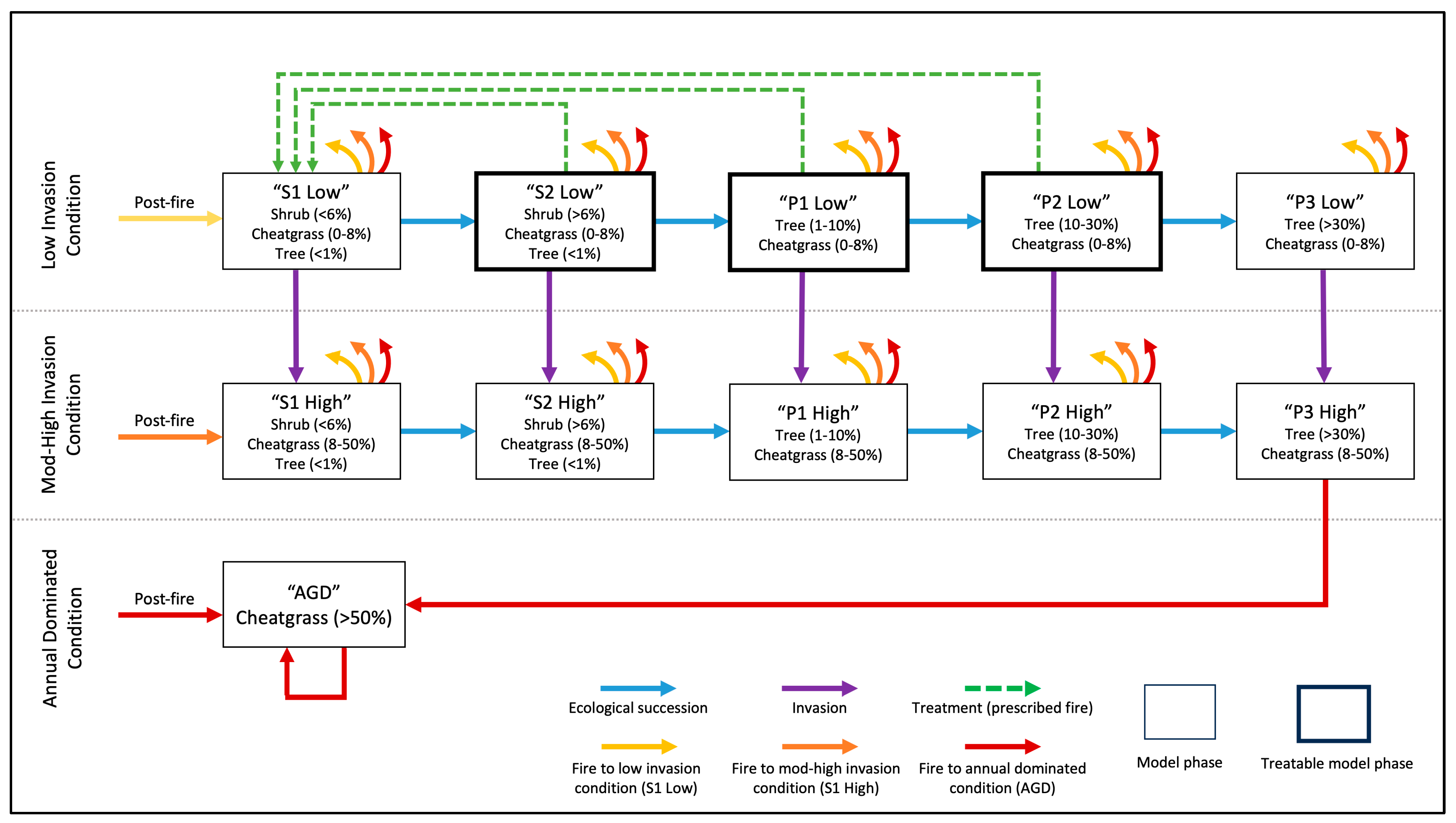
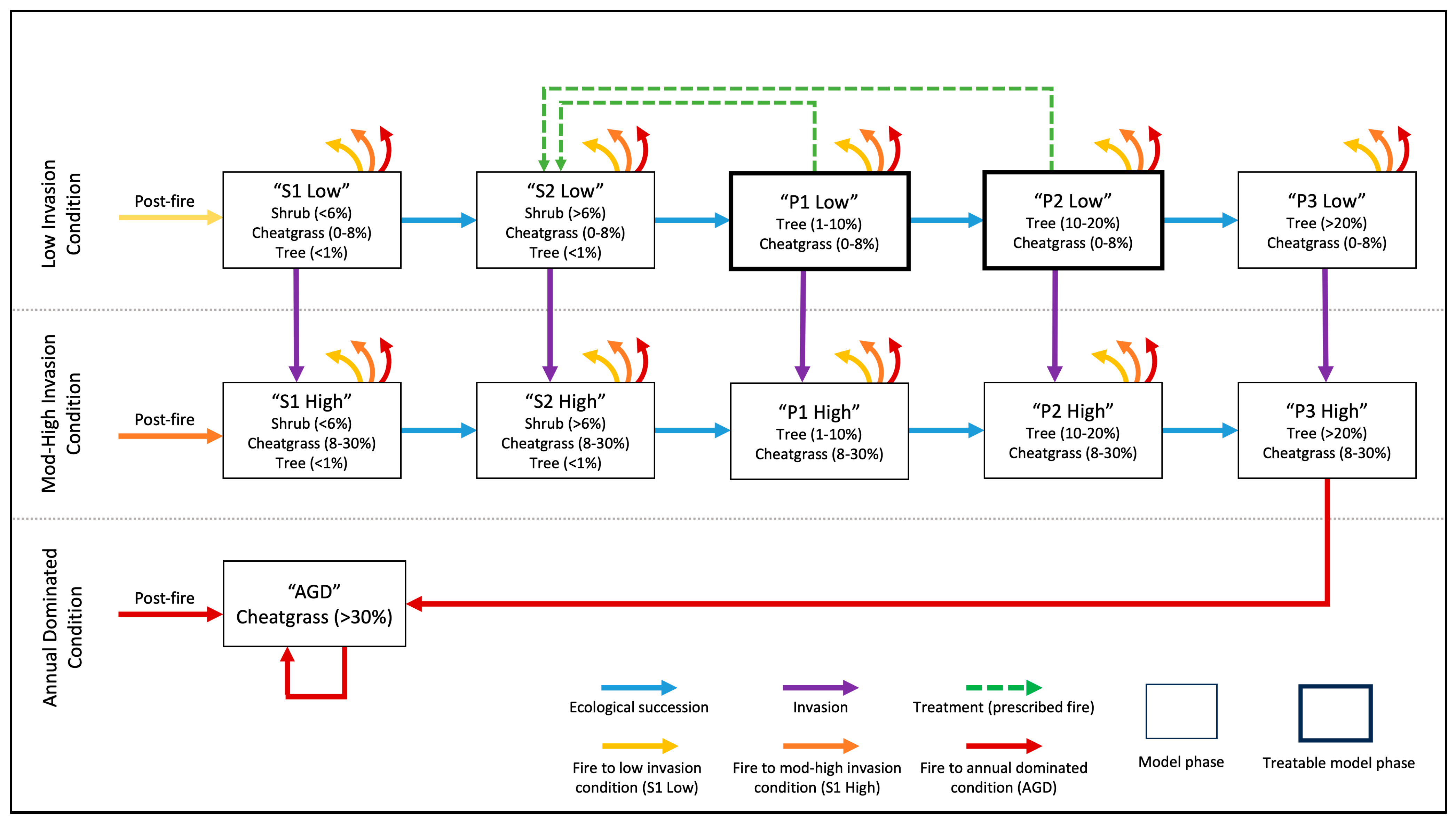
2.1. Dominant Sagebrush Associations

The study area matched the region for which TRGs were developed by Chambers et al. [18] and focused on three U.S. Environmental Protection Agency Level III ecoregions (Northern Basin and Range, Central Basin and Range, and Snake River Plain) in the Great Basin of the Western U.S. This study focused on three sagebrush vegetation associations within this region that experience both threats of annual grass invasion and PJ expansion: mountain big sagebrush, black sagebrush, and low sagebrush. Sagebrush associations within the study area covered 272,502 km², and these three sagebrush associations comprised 32% of that area [18].

2.2. Treatment Response Groups

For each dominant sagebrush association, this study considered the three TRGs with the largest areal extent as of 2020 that were likely to respond favorably to woody fuel treatments based on recent fuel modeling [9] and literature review [19]. Each TRG is characterized by a dominant sagebrush association, an indicator of resilience (RSL), and an indicator of resistance (RST), where the indicators take one of four values: low (L), moderate-low (ML), moderate (M), or high and moderate-high (H+MH). For each of the three sagebrush associations, the selected TRGs comprised over 80% of the association’s area in phases suitable for treatment (sagebrush only, Phase I, and Phase II woodland for mountain big sagebrush; Phase I and Phase II woodland for black sagebrush and low sagebrush;

Table 1. Treatment response groups (TRGs) for each dominant sagebrush association selected for this paper by recent areal extent (see text for details). For each TRG, the pre-smoothing cover area of the TRG in phases suitable for treatment (sagebrush only, Phase I, and Phase II woodland for mountain big sagebrush; Phase I and Phase II woodland for black sagebrush and low sagebrush) and the size of these areas relative to the total suitable treatment area for the dominant sagebrush within the study area were derived from Chambers et al. [18]. Each TRG corresponds to associations characterized by a dominant sagebrush association with particular levels of resilience and resistance indicators (RSL and RST, respectively). The four levels of the R&R indicators are low (L), moderate-low (ML), moderate (M), and high and moderate-high (H+MH).

Treatment Response Group (TRG)
Dominant Sagebrush Association	RSL	RST	Area of TRG Suitable for Treatment in 2020 (sq. km)	Relative Size of Area of TRG Suitable for Treatment in 2020 (%)
Mountain big sagebrush	M	M	12,266	45.7
Mountain big sagebrush	H+MH	H+MH	6491	24.2
Mountain big sagebrush	M	ML	3455	12.9
Black sagebrush	ML	ML	1804	60.3
Black sagebrush	M	ML	559	18.7
Black sagebrush	M	M	418	14.0
Low sagebrush	M	M	1521	52.7
Low sagebrush	ML	ML	504	17.5
Low sagebrush	ML	M	416	14.4

).

2.3. Generalized Treatment Response Models

For this study, generalized treatment response models (GTRMs) were developed to represent the broad dynamics of sagebrush ecosystems experiencing annual grass invasion and PJ expansion, which allowed for parameterizations to vary with levels of R&R. Drawing on the community phases and states that comprise the Cold Deserts state and transition models presented by Chambers et al. [20], the GTRMs described vegetation composition using discrete model phases, each of which was characterized by the composition of shrubs, trees, and annual grasses as determined by absolute vegetation cover percentages. The models included four types of pathways between model phases: ecological succession, fuel reduction treatment, wildfire, and invasion.

The GTRMs consisted of 11 model phases that fell into one of three invasion conditions depending on the absolute annual grass cover: low invasion, moderate to high (mod-high) invasion, and annual grass-dominated. The low invasion condition applied to sagebrush communities with 0–8% absolute cover of annual grass and corresponded to the “no-to-low” threat level defined by Doherty et al. [4]. This value, however, is below the 8–15% absolute cover of annual grass corresponding to the “growth” areas suitable for treatment by Doherty et al. [4] and used by Chambers et al. [18] to indicate areas currently suitable for treatment. The conservative lower value of 8% reflected the moderate to high risk of invasion occurring across much of the Great Basin [1,6,21] and the possibility that climate warming will likely increase the susceptibility of cooler and moister mountain big sagebrush, black sagebrush, and low sagebrush to annual grass invasion over the 100-year modeling timeframe [22,23]. The mod–high invasion condition applied to communities with an absolute annual cover over 8% and below the threshold for annual grass dominance, which depended on the dominant sagebrush association to reflect the productivity of these areas. Following recommendations from ecologists, for TRGs where mountain big sagebrush is the dominant sagebrush type, the model used 50% for the threshold above which the system was in the annual grass-dominated condition. For TRGs where black sagebrush and low sagebrush are the dominant sagebrush type, the model used a 30% threshold. The annual grass-dominated condition applied in each of these communities when absolute annual grass cover exceeded the respective thresholds.

The low invasion and mod–high invasion conditions were both comprised of five model phases: perennial dominant (“S1”), sagebrush dominant (“S2”), and three phases of woodland of increasing tree density, Phase I (“P1”), Phase II (“P2”), and Phase III (“P3”) following Miller et al. [2]. References to model phases in a specific invasion condition include “Low” or “High” in the name (e.g., “S1 Low”). The only model phase in the annual grass-dominated condition was the annual grass-dominated state (“AGD”).

Ecological succession between model phases in the low invasion and mod–high invasion conditions occurred deterministically after a certain number of years had elapsed in a model phase (Figure 1). Succession pathways in the low invasion and mod-high invasion conditions connected S1 to S2, S2 to P1, P1 to P2, and P2 to P3.

Fuel reduction treatments were applied only in the low invasion condition where the potential negative effects of treatments on invasive annuals were likely minimized. Prescribed fire could be applied in three model phases (S2, P1, and P2), and it forced a transition to S1 under the assumption of replacement severity fire. Cut-and-pile burn, applied only in Phase I and Phase II woodland (P1 and P2), preserved the understory and transitioned to S2. Following the treatment recommendations for each TRG [18], the models included prescribed fire treatment in the mountain big sagebrush GTRM and cut-and-pile burn treatment to remove trees in the black sagebrush and low sagebrush GTRM.

Wildfire could occur in any model phase. All wildfires were treated as replacement severity and transitioned the system to the earliest successional model phase in the destination condition (S1 Low in the low invasion condition; S1 High in the mod–high invasion condition; AGD in the annual condition). If wildfire occurred in the low invasion condition or the mod–high invasion condition, the system could transition to any of the three conditions. In the annual grass-dominated model phase, however, absent shrubs and trees pre-fire, the system remained in the annual grass-dominated model phase following fire.

The final type of pathway, invasion, represented transitions from the low invasion condition to the mod–high invasion condition when annual grass cover increased above 8%. Following invasion, the system moved from a model phase in the low invasion condition to the corresponding model phase in the mod–high invasion condition. Progression to the annual state required disturbance events that eliminated shrubs and trees and occurred only following wildfire.

The model phases and pathways between model phases in the ecological model were identical across all TRGs, with the exception of treatment pathways, which depended on whether prescribed fire or cut-and-pile burn was assigned. Figure 1 illustrates the model phases and transitional pathways in the GTRM for mountain big sagebrush systems; Figure 2 illustrates the GTRM for black sagebrush and low sagebrush systems. The parameters of each model, however, were allowed to differ between TRGs.

2.4. Ecological Parameters

2.4.1. Succession Times

To derive succession times for the parameterized GTRMs, the LANDFIRE biophysical setting (BpS) models most appropriate for the dominant sagebrush types of interest were identified: Inter-Mountain Basins Montane Sagebrush Steppe for mountain big sagebrush [24] and Great Basin Xeric Mixed-Sagebrush Shrubland for black sagebrush and low sagebrush [25]. As BpS models vary by region, this paper considered the BpS models that included LANDFIRE map zones 12, 17, and 18, which together cover the majority of the TRG study area.

For each dominant sagebrush type, baseline ecological succession times were identified from the deterministic model parameters in the BpS model descriptions. To ensure the times between model phases aligned with the BpS model parameters, a crosswalk between BpS succession classes and model phases (Table S1) was developed using the descriptions of succession classes’ vegetation composition from the BpS descriptions. The BpS deterministic model parameters provided all baseline succession times except for the transition from P2 to P3 for black sagebrush and low sagebrush. In this case, the baseline succession time corresponded to the succession time between succession classes B and C from the LANDFIRE PJ model appropriate to the study region [26].

As BpS models describe the dynamics of historical, undisturbed ecosystems, the baseline times were assigned to the low invasion condition in the TRG with moderate resilience and moderate resistance. A panel of experts (N = 3) in sagebrush wildfire ecology (the “Fire Risk Working Group”) modified the low invasion condition succession times for all other combinations of R&R. Typically, ecological succession takes longer in lower R&R classes, reflecting the community’s diminished capacity to recover. Constrained resource availability at higher elevations, however, can lengthen succession times at the highest levels of resilience and resistance. In the mod–high invasion condition, again following expert opinion from the Fire Risk Working Group, succession times were lengthened in areas with low R&R, as these areas are prone to increased invasion and longer succession times for woody plant recovery. Succession times in the mod–high invasion condition were derived by multiplying low invasion condition succession times by a factor, the mod–high multiplier, and rounding upward to the nearest integer when necessary.

Table 2. Succession times (years) by treatment response group (TRG) in the low invasion condition (0–8% absolute annual cover) and multipliers for adjusting succession times to the mod–high invasion condition (8–50% absolute annual cover for mountain big sagebrush; 8–30% for black sagebrush and low sagebrush). Low invasion succession times in the moderate resilience and moderate resistance (M/M) TRGs were assigned from LANDFIRE biophysical setting (BpS) model descriptions for Inter–Mountain Basins Montane Sagebrush Steppe [24] to mountain big sagebrush, Great Basin Xeric Mixed–Sagebrush Shrubland [25] to most succession times for black sagebrush and low sagebrush, and Great Basin Pinyon–Juniper Woodland [26] to low invasion P2 to P3 for black sagebrush and low sagebrush. Each TRG corresponds to a dominant sagebrush association with particular levels of resilience and resistance indicators (RSL and RST, respectively). The four levels of the R&R indicators are low (L), moderate-low (ML), moderate (M), and high and moderate-high (H+MH). The mod–high invasion multiplier is the factor used to scale for succession times in the mod–high invasion condition. For example, in simulations of mountain big sagebrush with moderate resilience and moderate resistance categories, succession from model phase S1 to model phase S2 took 12 years in the low invasion condition and 12 × 1.5 = 18 years in the mod–high invasion condition.

Treatment Response Group			Low Invasion Succession Times (Years)
Dominant Sagebrush Association	RSL	RST	S1 to S2	S2 to P1	P1 to P2	P2 to P3	Mod–High Multiplier
Mountain big sagebrush	H+MH	H+MH	20	50	45	51	1
Mountain big sagebrush	M	M	12	38	30	45	1.5
Mountain big sagebrush	M	ML	15	45	40	51	2
Black sagebrush	M	M	24	96	75	50	1.5
Black sagebrush	M	ML	29	101	80	55	2
Black sagebrush	ML	ML	34	106	85	60	2.5
Low sagebrush	M	M	24	96	75	50	1.5
Low sagebrush	ML	M	29	101	80	55	1.5
Low sagebrush	ML	ML	34	106	85	60	2.5

presents the succession times between model phases in the low invasion condition and the mod-high multipliers for the TRGs in this study.

2.4.2. Parameterization Regions

To find probability parameters associated with invasion, wildfire, and post-fire response specific to GTRM model phases, publicly available spatial data products were used to identify cells pertaining to the model phases of each TRG across the study region. Parameterization methods involving spatial data were performed in the R programming language [27] using the terra [28] and sf [29] packages.

Regions pertaining to each of the dominant sagebrush types were identified from the TRG raster data developed by Chambers et al. [18] and then masked to include only areas that fall within the LANDFIRE map zones [30] included in the dominant sagebrush type’s associated BpS model (Table S1). These regions did not include the mixed dominant sagebrush types (i.e., mixed low sagebrush combining black sagebrush and low sagebrush), areas where the PJ category was listed as “Not Sage” or “PJ Persistent Woodland”, or areas listed as rare combinations from Chambers et al. [18]. The further masking of these data by resilience and resistance indicators [14] produced the TRG extents used for parameterization.

The parameterization procedures described in Section 2.4.3, Section 2.4.4 and Section 2.4.5 relied upon identifying the model phase of cells in years 1990 and 2020. Model phases were identified from PJ categories from the TRG data [18] and from spatially explicit absolute foliar cover data from the Rangeland Analysis Platform v3 (RAP) [31]. To account for the high inter-annual variability in annual grasses and to be consistent in the treatment of each vegetation type, all vegetation data from RAP were averaged over five-year periods that led up to the year of interest (i.e., between 1986 and 1990 and between 2016 and 2020).

The invasion condition (low invasion, mod–high invasion, or annual grass-dominated) of the system was determined using RAP annual grasses and forbs cover. Each cell was assigned its invasion condition by comparing the average annual cover to the threshold definitions in Section 2.3.

Cells were assigned to PJ model phases (P1, P2, and P3) in 1990 by comparing the averaged RAP tree cover to the thresholds specified in Chambers et al. [18]. The TRG PJ category was used to differentiate between these woodland phases in 2020.

Cells were assigned to sagebrush model phases (S1 and S2) in 1990 if the averaged RAP tree cover was less than 1% and in 2020 if the TRG PJ category was “Sagebrush Only, No PJ”. To differentiate between the S1 and S2 model phases (both in 1990 and 2020), the averaged RAP shrub cover was compared to the threshold in the corresponding BpS model’s succession class descriptions. All thresholds for sagebrush model phases and PJ model phases are presented in

Table 3. Absolute vegetation cover thresholds for model phases and invasion conditions for each dominant sagebrush association. Shrub cover thresholds came from LANDFIRE biophysical setting (BpS) model descriptions [24,25]. Tree cover thresholds matched Chambers et al. [18]. All cover percentages below are in reference to absolute cover.

Dominant Sagebrush Association	Minimum Shrub Cover for S2	Minimum Tree Cover for P1	Minimum Tree Cover for P2	Minimum Tree Cover for P3	Minimum Annual Cover for Mod–High Invasion	Minimum Annual Cover for Annual Grass Dominant
Mountain big sagebrush	5%	1%	10%	30%	8%	50%
Black sagebrush	6%	1%	10%	20%	8%	30%
Low sagebrush	6%	1%	10%	20%	8%	30%

.

2.4.3. Invasion Probabilities

In the GTRMs, the system could move from one model phase in the low invasion condition to the corresponding model phase in the mod-high invasion condition absent the occurrence of fire. In the simulations, invasion was represented as an event with a yearly, time-invariant probability that varied with the TRG and with the current model phase but not with the length of time spent in-phase. As this transition occurred without wildfire, the invasion probabilities were conditional on wildfire not occurring in the same year.

The parameterization method for these probabilities analyzed cells that began in the low invasion condition in 1990 and did not experience a wildfire through 2020. For each TRG and for each model phase in the low invasion condition, the methods described in Section 2.4.2 identified the respective cells in 1990. Cells that experienced a fire between the years 1986 and 2020, determined using the Monitoring Trends in Burn Severity (MTBS) fire perimeter shapefile [32], were then excluded. The no-burn period began in 1986, so that the assessment of the invasion condition in 1990 was built upon a five-year average of annual cover in a relatively static community.

Of the qualifying cells, the percentage of cells that remained in the low invasion condition was computed, which served as an estimate of the probability that invasion did not occur in each year of a 30-year period. Under the assumptions that annual probabilities were time-invariant and that ecological succession did not occur during the 30-year period, $c_{Ref,30Y}$, the percentage of cells that remained in the low invasion condition after 30 years of no wildfire was related to the yearly probability of invasion conditional on no wildfire, $p_{inv}$, as described in Equation (1):

$$c_{Ref,30Y}\approx {\left(1-p_{inv}\right)}^{30}$$

(1)

Rewriting the above expression yielded the expression for the yearly invasion probability using the observed percentage $c_{Ref,30Y}$:

$${\widehat{p}}_{inv}=1-c_{Ref,30Y}^{{\displaystyle \frac{1}{30}}}$$

(2)

Equation (2) was used to estimate the invasion probability parameters (

Table 4. Probabilities of annual grass invasion in years without fire by treatment response group (TRG) and by generalized treatment response model (GTRM) model phases (S1 Low, S2 Low, P1 Low, P2 Low, and P3 Low) in the low invasion condition. Each probability listed below indicates the probability of transitioning from the low invasion condition model phase to the respective moderate to high invasion condition model phase in each year that fire did not occur. The number of 30 m × 30 m (0.09 hectares) cells that contributed to each probability estimate is indicated in parentheses below each estimate. Each TRG corresponds to associations characterized by a dominant sagebrush association with particular levels of resilience and resistance indicators (RSL and RST, respectively). The four levels of the R&R indicators are low (L), moderate-low (ML), moderate (M), and high and moderate-high (H+MH).

Treatment Response Group			Probability of Annual Grass Invasion by Model Phase
Dominant Sagebrush Type	RSL	RST	S1 Low	S2 Low	P1 Low	P2 Low	P3 Low
Mountain big sagebrush	H+MH	H+MH	0.004 (21,044)	0.012 (2,568,187)	0.007 (1,685,481)	0.002 (175,657)	0.000 (26,358)
Mountain big sagebrush	M	M	0.019 (10,305)	0.027 (4,114,602)	0.014 (1,765,492)	0.002 (464,496)	0.000 (178,968)
Mountain big sagebrush	M	ML	0.018 (6496)	0.032 (959,098)	0.017 (605,670)	0.002 (353,119)	0.000 (174,754)
Black sagebrush	M	M	0.005 (101)	0.025 (272,357)	0.007 (143,919)	0.001 (121,974)	0.000 (288,977)
Black sagebrush	M	ML	0.002 (145)	0.022 (184,577)	0.007 (360,624)	0.001 (272,130)	0.000 (592,077)
Black sagebrush	ML	ML	0.001 (1092)	0.030 (466,836)	0.010 (1,064,943)	0.002 (886,006)	0.001 (2,538,017)
Low sagebrush	M	M	0.010 (224)	0.026 (3,508,371)	0.014 (324,123)	0.005 (63,614)	0.002 (40,363)
Low sagebrush	ML	M	0.004 (249)	0.033 (859,610)	0.015 (111,744)	0.004 (21,270)	0.002 (15,664)
Low sagebrush	ML	ML	0.001 (631)	0.016 (1,396,097)	0.009 (138,317)	0.004 (16,677)	0.001 (17,822)

).

2.4.4. Wildfire Probabilities

Current annualized probabilities of wildfire impacts were derived from the raster dataset produced by FSim and calibrated to the sagebrush biome by Short et al. [33]. As these data reflect present fire likelihood (i.e., circa 2020 landscape, recent 15-year burn history) under current wildfire suppression practices, they do not represent true long-term burn probabilities or fire return intervals for each cell in the raster.

The parameterization of burn probabilities for each model phase in each TRG required the assumption that the yearly probability of wildfire occurrence could be approximated as the expected percentage of cells in the study region burned in a year in the current landscape. The burn probability raster was projected into a 30 m × 30 m resolution to match the other spatial datasets. As the data by Short et al. [33] originally had a resolution of 270 m × 270 m (7.29 hectares), the burn probability parameters in this study represented an expected yearly probability of wildfire in a 270 m × 270 m (7.29 hectares) area belonging to a particular TRG and model phase.

For model phases in the low invasion and high invasion conditions, the method described in Section 2.4.2. identified cells pertaining to each model phase in 2020 for each TRG. As AGD sites might not be classified under a dominant sagebrush type in the TRG data [18], for each sagebrush type, AGD model phases in each TRG were identified by considering all cells in the study region that were assigned the biophysical setting associated with the dominant sagebrush type in the relevant map zones using the LANDFIRE v2.0.0 biophysical setting raster and map zone shapefile [30] and masking the resulting raster to include only the cells that belonged to the level of R&R associated with the TRG and where the five-year average of RAP annual cover between 2016 and 2020 exceeded the annual condition threshold (Table 3). The yearly burn probability parameters are presented in

Table 5. Yearly burn probabilities by treatment response group (TRG) and by generalized treatment response model (GTRM) model phase. The number of 30 m × 30 m (0.09 hectares) cells that contributed to each estimate is provided in parentheses. Each TRG corresponds to associations characterized by a dominant sagebrush association with particular levels of resilience and resistance indicators (RSL and RST, respectively). The four levels of the R&R indicators are low (L), moderate-low (ML), moderate (M), and high and moderate-high (H+MH).

Treatment Response Group			Yearly Burn Probability by Model Phase
Dominant Sagebrush Association	RSL	RST	S1 Low	S2 Low	P1 Low	P2 Low	P3 Low	S1 High	S2 High	P1 High	P2 High	P3 High	AGD
Mountain big sagebrush	H+MH	H+MH	0.002 (6576)	0.009 (637,954)	0.014 (3,044,988)	0.014 (152,195)	0.006 (55,769)	0.013 (8345)	0.018 (692,014)	0.019 (1,794,137)	0.017 (19,279)	0.018 (1566)	0.018 (13,115)
Mountain big sagebrush	M	M	0.010 (12,062)	0.012 (1,016,675)	0.015 (2,620,086)	0.011 (296,685)	0.005 (403,806)	0.018 (123,998)	0.018 (3,267,612)	0.022 (3,501,617)	0.020 (44,920)	0.017 (5527)	0.024 (160,501)
Mountain big sagebrush	M	ML	0.008 (8497)	0.010 (266,122)	0.014 (592,957)	0.006 (213,947)	0.005 (367,142)	0.019 (107,790)	0.019 (971,881)	0.019 (1,208,102)	0.015 (24,761)	0.014 (4160)	0.018 (257,337)
Black sagebrush	M	M	0.018 (82)	0.007 (103,337)	0.007 (89,363)	0.005 (15,022)	0.005 (465,925)	0.024 (1525)	0.011 (172,359)	0.011 (69,847)	0.009 (1316)	0.009 (12,170)	0.019 (1,320,757)
Black sagebrush	M	ML	0.010 (230)	0.006 (58,554)	0.005 (224,592)	0.003 (77,636)	0.005 (919,126)	0.018 (1056)	0.011 (73,203)	0.007 (128,906)	0.006 (5622)	0.010 (30,137)	0.018 (491,922)
Black sagebrush	ML	ML	0.017 (2353)	0.006 (140,552)	0.005 (650,619)	0.005 (383,213)	0.006 (3,323,369)	0.019 (1363)	0.009 (146,812)	0.006 (610,874)	0.008 (39,776)	0.010 (95,451)	0.012 (452,398)
Low sagebrush	M	M	0.009 (1417)	0.005 (1,501,118)	0.007 (439,902)	0.006 (19,582)	0.012 (75,559)	0.018 (29,329)	0.008 (2,429,600)	0.011 (767,550)	0.012 (3221)	0.015 (7676)	0.019 (1,320,757)
Low sagebrush	ML	M	0.002 (151)	0.003 (244,800)	0.005 (157,516)	0.004 (10,472)	0.005 (22,851)	0.014 (1586)	0.005 (514,363)	0.008 (255,869)	0.005 (1384)	0.005 (626)	0.011 (152,977)
Low sagebrush	ML	ML	0.000 (1118)	0.004 (827,868)	0.004 (203,109)	0.005 (6543)	0.006 (21,458)	0.013 (4615)	0.006 (667,988)	0.007 (180,846)	0.007 (862)	0.007 (527)	0.012 (452,398)

.

2.4.5. Post-Fire Response

For all model phases in the GTRM, wildfire transitioned the system to either S1 in the low invasion condition, S1 in the mod–high invasion condition, or AGD in the annual grass-dominated condition. As fire severity and pre-fire perennial cover are both important factors in the post-fire recovery of sagebrush communities [7,8,11,34], the model allowed the post-fire probabilities of transitioning to each of these invasion conditions to change with the pre-fire model phase of the system.

The parameterization procedure looked at historical wildfire and quantified the percentage of cells that converted to each invasion condition after experiencing a single wildfire. The procedure described in Section 2.4.2. identified areas belonging to a combination of TRG and model phase in 1990. The MTBS fire perimeter shapefile was then used to identify the subarea that experienced a single wildfire between 1991 and 2005, excluding areas that did not burn during this period, burned multiple times, or may have burned intentionally for reasons potentially related to favorable recovery. To allow sufficient time for post-fire vegetation to recover, areas that burned after 2006 were removed. The process of erasing areas that experienced multiple burns produced slivers potentially related to the scale of precision in the shapefile perimeters, so a negative buffer of 60 m was applied to the single-burn shapefile mask to prevent the inclusion of boundary areas that might not have satisfied the aforementioned criteria for computing post-fire probabilities.

The post-fire probability distributions that resulted from the parameterization process are presented in Tables S2–S4. The number of cells that satisfied the parameterization criteria varied with TRG and with model phase. To account for consistently low qualifying cell counts in the S1 model phases in the low and mod–high invasion conditions, for each TRG, post-fire transition probabilities for the S1 and S2 model phases were determined from conversion rates after combining the S1 and S2 data. In two cases, P2 High in M/M black sagebrush and P2 High in ML/M low sagebrush, no cells qualified. The parameters for these two cases were assigned the probabilities associated with the same model phase in the TRG with the next highest R&R available (M/ML black sagebrush and M/M low sagebrush, respectively).

In two model phases, post-fire transitions were deterministic. First, following a fire in the AGD model phase, the system stayed in the AGD model phase under the assumption that the recovery of native vegetation was unlikely. Second, fire in mod–high invasion Phase III woodland forced a transition to the annual-dominated state. This transition assumed that mod–high invaded Phase III woodland had a depleted perennial understory that also was unlikely to recover following wildfire. This second assumption was again necessary since the restrictions used for parameterization resulted in small sample sizes (Tables S2–S4).

2.5. Economic Parameters

2.5.1. Treatment Costs

The per-acre costs of treatment were from the NRCS Environmental Quality Incentives Program (EQIP) payment schedules for Nevada in 2023 [35]. The cost per acre for prescribed fire of USD 16.58 per acre (USD 40.97 per hectare) was specific to steep terrain, and the cost of pile-and-burn, USD 275.47 per acre (USD 680.69 per hectare), was assumed to be inclusive of all activities required for the treatment practice. To prevent inflating benefit–cost ratios, the most expensive estimate among relevant alternatives was used. Treatment costs varied only with treatment type, not with the initial model phase or the TRG in which treatment was applied. While there can be a large variability in treatment costs depending on site characteristics (e.g., vegetation, slope, proximity to roadways), these estimates were conservative and avoided overstating the benefits of treatment.

2.5.2. Wildfire Suppression Costs

Wildfire suppression cost data came from a subset of a USDA Forest Service (FS) dataset that resolved potential overlaps in federal agency accounting and reported sizes, National Fire Danger Rating System (NFDRS) fuel models at the point of ignition, and combined federal expenditures on wildfires following the methods developed by Gebert et al. [36]. The same data were used for Taylor et al. [16] and Taylor et al. [17] and included information on 3152 wildfires across all FS regions between 1995 and 2013. Observations without information on total expenditure, acreage, or NFDRS fuel model (N = 14) and observations with a category label including the term “reject” (N = 43) were removed. For each NFDRS fuel model, outliers were identified and removed where the per-acre wildfire suppression cost fell two sample standard deviations above or below the sample mean for the fuel model (N = 119). Cost data were converted into 2023 dollars using the Government Consumption Expenditures and Gross Investment: Federal: Non-Defense price index [37].

The model phases in the GTRMs were matched to NFDRS fuel models by adapting the crosswalk used in Taylor et al. [16] derived from fuel model descriptions by Anderson [38]. The simulation code assessed the cost of wildfire suppression for a particular model phase by sampling per-hectare wildfire suppression costs from the observations in the FS expenditure dataset pertaining to the associated fuel model. As wildfires vary widely in area, a burned cell is more likely to belong to a large wildfire than a small wildfire. Per-acre wildfire suppression costs were sampled from the FS expenditure data weighting by the area of each fire.

Of the 2976 observations in the cleaned FS wildfire suppression cost data, 1069 observations pertained to the five NFDRS models that appeared in the crosswalk. Table S5 reports the model phase–NFDRS model crosswalk and the mean and median per-hectare wildfire suppression costs associated with each NFDRS fuel model.

2.5.3. Additional Economic Benefits of Intact Sagebrush

Cornachione et al. [39] studied PJ removal in mountain big sagebrush sites in central Nevada and through benefit transfer derived per-acre increases in ecosystem value associated with a lop-and-scatter treatment. Combining their estimated net present values of benefits to grazing, water availability, greater sage-grouse habitat, and recreation/hunting, and excluding wildfire suppression cost savings, these public economic benefits of treatment amount to USD 105 per acre (USD 259.46 per hectare), which is equivalent to USD 5.36 per acre (USD 13.24 per hectare) for each of the 30 years with a 3% discount rate. As a lop-and-scatter technique would not remove the sagebrush understory, USD 13.24 served as a rough approximation of the yearly per-hectare value of an intact sagebrush-dominated (i.e., S2) mountain big sagebrush community relative to Phase II woodland (i.e., P2), the model phase that best characterized the study area in Cornachione et al. [39].

2.6. Simulation

The simulation platform was written in R [27], adapting the code used for state and transition model simulation by Taylor et al. [17] to accommodate the model phases and invasion conditions of the GTRMs, to allow parameter sets to vary with TRGs, and to allow for invasion transitions between low invasion condition and mod-high invasion condition model phases. Parameters entered the simulation code through input spreadsheets, and scripts processed the output to produce tables of ecological and economic results for both treatment and non-treatment scenarios.

Each simulation consisted of 50,000 runs. Each run followed a parameterized GTRM to simulate ecological dynamics across a management horizon of 100 years. To reflect fuel treatment decisions by land managers, for each TRG, simulations ran under treatment and no treatment scenarios for initializations in each treatable model phases: low invasion S2, P1, and P2 for prescribed fire models in mountain big sagebrush systems, and low invasion P1 and P2 for mechanical treatment models in black sagebrush and low sagebrush systems. To reflect uncertainty regarding how long the system may have been in the initial model phase, the years already spent in the initial model phase were assumed to be uniformly distributed across the number of years until succession to the next model phase (Table 2).

The occurrence of stochastic events was determined by random numbers sampled from a continuous uniform distribution between 0 and 1 that were generated for each year in the run for each event. For a random event of type $e$ with probability $p$, the event would occur in year $t$ of run $m$ if the respective sample from the standard uniform distribution, ${\widehat{p}}_{ept}$, was less than $p$. For each year, the simulation first determined if a fire occurred. If no fire occurred, treatment could be applied. If no fire or treatment occurred, the simulation allowed first for ecological succession and then for invasion absent fire. Ecological succession occurred deterministically after the years specified in Table 3 elapsed. When invasion moved the system into a mod–high invasion model phase, the succession clock preserved the progress toward succession already made in the previous model phase as a percentage of succession time to the next model phase. The outcomes of these events determined the invasion condition and model phase in the next year.

For each combination of TRG and initial model phase, simulations were performed with treatment and with no treatment. To make the treatment and no treatment scenarios comparable, each treatment/no treatment pair of simulations shared the same random number generator seed and, accordingly, all realized event probability samples ${\widehat{p}}_{ept}$. In the treatment scenario, treatment occurred in the first year if fire did not occur. Retreatment could occur if the system reached the last year of the low invasion S2 model phase in the case of prescribed fire or the first year of the low invasion P1 model phase in the case of cut-and-pile burn.

To compute benefit–cost ratios, the net present value (NPV) of a fuel treatment’s benefits over a time horizon, $T$, was derived from the incidences of events in the generated ecological trajectories. For run $m$ of a simulation, the NPV of benefits was the difference in the present value (PV) of benefits under the treatment scenario, $PV\left(B^{m,TREAT}\right)$, and the present value of benefits under the no treatment scenario, $PV\left(B^{m,NOTREAT}\right)$. Following Equation (3), these present values under a treatment or no treatment scenario, $s$, were calculated as the sum of the benefits in each year of the simulation run, $B_t^{m,s},$ discounted at a rate of $r=$ 3% per year as per Loomis [40]:

$$PV\left(B^{m,s}\right)=\sum _{t=0}^{T-1}{\displaystyle \frac{1}{{\left(1+r\right)}^t}}{B}_t^{m,s}$$

(3)

Two different assessments of benefits were considered. The first method only incorporated wildfire suppression cost savings, in which case the benefit at time $t$ was 0 less the wildfire suppression cost in year $t$. The second method for assessing the benefits of treatment additionally incorporated the value of preserving intact sagebrush ecosystems as determined by Cornachione et al. [39]. For each year in the treatment scenario, the benefit of PJ removal was added if the treatment scenario was in a low invasion condition sagebrush model phase (S1 or S2) and the non-treatment scenario was in any PJ model phase (P1–P3 in either low invasion or mod-high invasion conditions). The value of preserving intact sagebrush was subtracted if the treatment scenario was characterized by PJ and the non-treatment scenario was in a low invasion sagebrush model phase.

Next, the net present value of treatment costs across the management time horizon for each run, $m$, was the present value of treatment costs in the treatment scenario, $TreatCos{t}^{m,Treat}$. Allowing for retreatment and denoting the treatment costs in year $t$ as $TreatCos{t}_t^{m,TREAT}$, the present value of treatment costs was calculated following Equation (4):

$$PV\left(TreatCos{t}^{m,TREAT}\right)=\sum _{t=0}^{T-1}{\displaystyle \frac{1}{{\left(1+r\right)}^t}}{TreatCost}_t^{m,Treat}$$

(4)

Averaging across all runs in a simulation yielded the expected net present value of treatment benefits and costs. Following Equation (5), dividing the expected net present value of treatment benefits by the expected net present value of treatment costs produced the estimated benefit–cost ratio:

$$\widehat{E\left[BCR\right]}={\displaystyle \frac{\frac{1}{50000}{\sum }_{m=1}^{50000}PV\left(B^{m,TREAT}\right)-\frac{1}{50000}{\sum }_{m=1}^{50000}PV\left(B^{m,NOTREAT}\right)}{\frac{1}{50000}{\sum }_{m=1}^{50000}PV\left(TreatCos{t}^{m,TREAT}\right)}}$$

(5)

3. Results

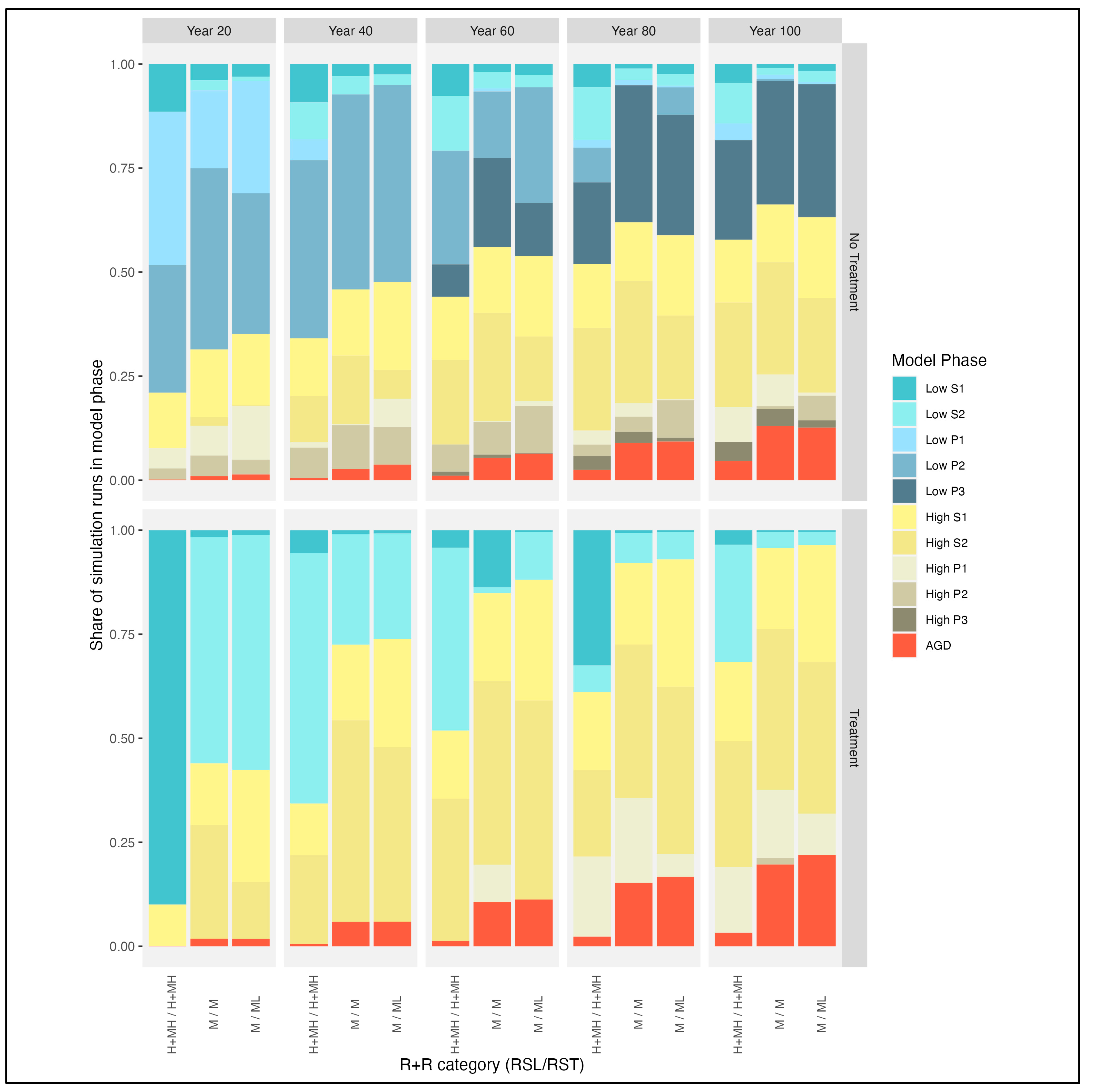
3.1. Mountain Big Sagebrush

3.1.1. Ecological Outcomes

Ecological trade-offs were inherent to fuel treatments in the mountain big sagebrush simulations (Figure 3,

Table 6. Ecological outcomes for mountain big sagebrush TRGs from the 100-year simulations. The first row indicates the model phase in the low invasion condition in which simulation began. “Treat” indicates prescribed fire occurred in the first year of simulation if wildfire did not occur. Treatment response groups (TRGs) are identified by resilience (RSL) and resistance (RST) indicators. The four levels of the R&R indicators are low (L), moderate-low (ML), moderate (M), and high and moderate-high (H+MH).

	Initial Model Phase
	S2	S2	S2	P1	P1	P1	P2	P2	P2
	RSL/RST
	H+MH/ H+MH	M/M	M/ML	H+MH/ H+MH	M/M	M/ML	H+MH/ H+MH	M/M	M/ML
No Treat: Proportion of simulation runs ending in low invasion model phases	0.29	0.15	0.12	0.42	0.34	0.37	0.62	0.54	0.59
No Treat: Proportion of simulation runs ending in mod–high invasion model phases	0.68	0.69	0.68	0.53	0.53	0.51	0.34	0.36	0.32
No Treat: Proportion of simulation runs ending in annual grass-dominated model phase	0.04	0.16	0.20	0.05	0.13	0.13	0.04	0.10	0.08
No Treat: Proportion of simulation runs ending in sagebrush model phases	0.62	0.55	0.57	0.54	0.44	0.46	0.42	0.32	0.32
No Treat: Proportion of simulation runs ending in woodland model phases	0.34	0.29	0.23	0.41	0.43	0.41	0.54	0.58	0.59
No Treat: Mean total number of wildfires	1.33	1.67	1.63	1.28	1.43	1.28	1.00	1.01	0.81
Treat: Proportion of simulation runs ending in low invasion model phases	0.31	0.04	0.03	0.32	0.04	0.04	0.31	0.04	0.03
Treat: Proportion of simulation runs ending in mod–high invasion model phases	0.65	0.76	0.75	0.65	0.76	0.74	0.65	0.76	0.75
Treat: Proportion of simulation runs ending in annual grass-dominated model phase	0.03	0.20	0.22	0.03	0.20	0.22	0.03	0.20	0.22
Treat: Proportion of simulation runs ending in sagebrush model phases	0.81	0.63	0.68	0.81	0.62	0.68	0.81	0.62	0.68
Treat: Proportion of simulation runs ending in woodland model phases	0.16	0.18	0.10	0.16	0.18	0.10	0.16	0.18	0.10
Treat: Mean total number of wildfires	0.99	1.64	1.59	1.00	1.64	1.59	1.00	1.64	1.57

). Consistent with the goals of treatment, treated TRGs were more likely to be in sagebrush model phases (S1 and S2) and less likely to be in PJ woodland phases (P1, P2, and P3) than untreated TRGs. Figure 3 illustrates this outcome over the 100-year planning horizon when the initial phase was P1. Table 6 shows that treated TRGs were more likely to be in a sagebrush model phase at the end of the planning horizon compared to untreated TRGs, particularly when the model started in a PJ woodland phase (P1 or P2). Conversely, only a relatively small fraction of treated TRGs were in a PJ woodland model phase at the end of the planning horizon (between 10–18%), while in untreated simulations, depending on the TRG, between 23–34% of runs ended in a PJ woodland phase when the initial model phase was S2, 41–43% when the initial phase was P1, and 54–59% when the initial phase is P2.

While treatment was successful at tilting the system towards sagebrush model phases and away from PJ woodland phases, in all simulations other than the H+MH/H+MH system initialized in S2, treatment increased the likelihood that that TRGs transitioned out of the low invasion condition and into the mod–high and annual grass-dominated invasion conditions (Figure 3, Table 6). Treatment increased annual grass invasion because the invasion probability parameters were highest for S2 and lowest for P2 and P3 (Table 4). Transitions to the mod–high invasion condition increased both the wildfire frequency (Table 5) and the likelihood that the system transitioned to the annual grass-dominated phase post-fire.

The impact of treatment on the mean number of wildfires over the 100-year planning horizon was related to the influence of the treatment on annual grass invasion. When the initial model phase was S2, treatment led to a small reduction in the mean number of wildfires in all TRGs. This result stems from the fact that when the initial model phase was S2, treatment had a modest impact on annual grass invasion and, hence, wildfire activity, relative to the no treatment case. When the initial phase was P1 or P2, however, treatment increased the relative probability of annual grass invasion in the short term and, as a result, increased wildfire occurrence in all instances except for the highest R&R TRG (H+MH/H+MH) simulations.

The ecological outcomes in the mountain big sagebrush simulations varied with R&R (Figure 3, Table 6). Independent of treatment, simulation runs for the TRG with the highest level of R&R (H+MH/H+MH) experienced much lower invasion rates in the post-treatment model phase S1 (Table 4) and were more likely to remain in the low invasion condition. Concerning the impact of R&R on the long-term efficacy of treatment, for the highest R&R TRG, over 80% of model runs in treatment scenarios remained in sagebrush phases (S1 and S2) through the planning horizon in all three initial phases, compared to between 62% and 68% of model runs for lower R&R TRGs (Table 6). In the highest R&R TRG, treatment reduced the number of wildfires when the initial phase was S2 and P1 and only led to a negligible change in wildfire when the initial phase was P2 (Table 6). By contrast, in the two lower R&R TRGs, treatment led to small reductions in the mean number of wildfires when the initial phase was S2 and increased the number of wildfires when the initial phase was P1 or P2.

3.1.2. Economic Outcomes

Fuel reduction treatments resulted in positive wildfire suppression cost savings in the mountain big sagebrush simulations in all initializations (

Table 7. Economic outcomes for mountain big sagebrush TRGs from 100-year simulations. The first row indicates the model phase in the low invasion condition in which simulation began. “Treat” indicates prescribed fire occurred in the first year of simulation if wildfire did not occur and retreatment could occur. Treatment response groups (TRGs) are identified by resilience (RSL) and resistance (RST) indicators. The four levels of the R&R indicators are low (L), moderate-low (ML), moderate (M), and high and moderate-high (H+MH).

	Initial Model Phase
	S2	S2	S2	P1	P1	P1	P2	P2	P2
	RSL/RST
	H+MH/ H+MH	M/M	M/ML	H+MH/ H+MH	M/M	M/ML	H+MH/ H+MH	M/M	M/ML
No Treat: Mean cost of wildfire suppression per hectare (USD; PV)	268.92	341.77	305.37	357.19	376.76	320.08	319.03	280.16	200.98
Treat: Mean cost of wildfire suppression per hectare (USD; PV)	121.58	225.88	190.27	130.26	231.99	193.01	129.67	226.86	191.73
Treat: Mean wildfire suppression cost savings per hectare (USD; NPV)	147.34	115.89	115.10	226.93	144.76	127.07	189.36	53.30	9.25
Treat: Mean PJ removal benefits per hectare (USD)	98.57	72.32	59.27	257.83	199.56	201.59	270.09	208.89	215.40
Treat: Mean combined benefits per hectare (USD)	245.91	188.21	174.38	484.76	344.33	328.66	459.45	262.19	224.65
Treat: Mean number of treatments	1.32	1.16	1.10	1.31	1.16	1.09	1.31	1.16	1.10
Treat: Mean cost of treatment per hectare (USD; PV)	42.26	42.14	41.30	42.06	41.94	41.17	42.08	42.12	41.46
Treat: Mean benefit–cost ratio (wildfire costs only)	3.49	2.75	2.79	5.40	3.45	3.09	4.50	1.27	0.22
Treat: Mean benefit–cost ratio (total benefits)	5.82	4.47	4.22	11.52	8.21	7.98	10.92	6.22	5.42

). Depending on the TRG, the net present value of suppression cost savings ranged from USD 115 to USD 147 per hectare when the initial phase was S2, from USD 127 to USD 227 when the initial phase was P1, and from USD 9 to USD 189 when the initial phase was P2.

Treatment reduced wildfire suppression costs early in the planning horizon because yearly burn probabilities (Table 5) and mean per-acre wildfire suppression costs (Table S5) were mostly lower in the post-treatment phase, S1, than in any of the three initial phases (S2, P1, and P2). For all initializations of the H+MH/H+MH TRG, the suppression cost savings early in the planning horizon, without any large increases in the number of wildfires and with low conversion to the annual grass-dominated state across the entire planning horizon, led to wildfire suppression cost savings. In the case of the S2 initializations of the M/M and M/ML simulations, the early savings and the reduction in wildfires offset the potential for more costly fires in the annual grass-dominated state late in the planning horizon. For the P1 and P2 initializations of M/M and M/ML, while treatment led to 15–94% increases in wildfire occurrence over the planning horizon, the early savings still produced positive wildfire suppression cost savings. The wildfire suppression cost savings with fuel treatment were increasing with R&R (Table 7).

The benefits from preserving intact sagebrush systems (i.e., the benefits from the system being in a sagebrush model phase in the low invasion condition relative to a pinyon–juniper woodland model phase; see Section 2.4.3) were largest in the highest R&R TRG. This result can be explained by lower invasion rates and the fact that the highest succession times occurred in the highest R&R TRG. For all initializations of the lower R&R TRGs (M/M and M/ML), the preservation benefits were similar in magnitude and differed by a maximum of USD 13 in the S2 initialization. While benefits from preserving intact sagebrush systems were highest when initial treatment moved the system from a PJ woodland model phase (P1 and P2) into the first sagebrush model phase (S1), treatments also generated these benefits when the initial model phase was S2 by extending the time to transition to a PJ woodland model phase through ecological succession.

All TRGs had benefit–cost ratios (BCRs) that were greater than one based on wildfire suppression costs savings alone when the initial phase was S2 or P1, suggesting that, on average, suppression cost savings covered the cost of treatment in these phases (Table 7). The H+MH/H+MH and M/M TRGs also had a BCR greater than one based on wildfire suppression cost savings when the initial phase was P2. The BCRs further increased when the additional (non-wildfire-related) benefits from preserving intact sagebrush systems were included, causing all TRGs to have BCRs greater than one in all initializations.

BCRs incorporating only wildfire suppression cost-saving benefits were highest in the H+MH/H+MH TRG for each of the three initial model phases, and these BCRs were increasing with R&R in the P1 and P2 initializations. BCRs incorporating non-wildfire-related benefits were all increasing with R&R, though differences in BCRs between the lower R&R TRGs (M/M and M/ML) were relatively small.

Compared to the black sagebrush and low sagebrush systems considered below, the larger BCRs in the mountain big sagebrush simulations (Table 7) were attributable to the low per-acre cost of treating with prescribed fire. While the model allowed for repeated treatments, follow-up treatments occurred far out in the planning horizon (50+ years) and, therefore, received little weight in calculations of the NPV of treatment cost. For this reason, the NPV of treatment cost was close to the USD 40.97 per hectare treatment cost borne in the first period.

3.2. Black Sagebrush

Similar to the mountain big sagebrush results, mechanical fuel treatments in black sagebrush simulations made sagebrush model phases more likely and PJ woodland phases less likely, but also increased the likelihood of transitions to the mod–high invasion condition and the annual grass-dominated phase (

Table 8. Ecological and economic outcomes for black sagebrush TRGs from 100-year simulations. The first row indicates the model phase in the low invasion condition in which simulation began. “Treat” indicates cut-and-pile burn occurred in the first year if wildfire did not occur and retreatment could occur. Treatment response groups (TRGs) are identified by resilience (RSL) and resistance (RST) indicators. The four levels of the R&R indicators are low (L), moderate-low (ML), moderate (M), and high and moderate-high (H+MH).

	Initial Model Phase
	P1	P1	P1	P2	P2	P2
	RSL/RST
	M/M	M/ML	ML/ML	M/M	M/ML	ML/ML
No Treat: Proportion of simulation runs ending in low invasion model phases	0.48	0.53	0.41	0.67	0.68	0.56
No Treat: Proportion of simulation runs ending in annual grass-dominated model phase	0.18	0.12	0.17	0.12	0.12	0.17
Treat: Proportion of simulation runs ending in low invasion model phases	0.05	0.08	0.04	0.05	0.08	0.04
Treat: Proportion of simulation runs ending in annual grass-dominated model phase	0.36	0.27	0.33	0.36	0.27	0.33
No Treat: Mean cost of wildfire suppression per hectare (USD; PV)	216.31	147.68	170.85	178.24	155.80	203.51
Treat: Mean cost of wildfire suppression per hectare (USD; PV)	192.57	161.64	156.96	187.75	162.13	157.81
Treat: Mean wildfire suppression cost savings per hectare (USD; NPV)	23.74	−13.96	13.89	−9.51	−6.33	45.70
Treat: Mean benefit–cost ratio (wildfire costs only)	0.04	−0.02	0.02	−0.01	−0.01	0.07

; Tables S6 and S7 contain full ecological and economic outcomes for black sagebrush). Also similar to the M/M and M/ML mountain big sagebrush simulations initialized in P1 and P2, treatment in the black sagebrush simulations increased the mean number of wildfires over the 100-year planning horizon because higher invasion rates in S2 contributed to annual grass invasion and increased wildfire occurrence in the long term. Under treatment, higher R&R categories experienced more frequent wildfire.

The effect of fuel treatments on wildfire suppression costs in the black sagebrush system varied by TRG and by initialization. While the mechanism for wildfire suppression cost savings in the black sagebrush system was the same as in mountain big sagebrush, the lower suppression costs associated with wildfire in the earlier model did not always compensate for the increase in wildfire occurrence in the short term and the increase in expected wildfire suppression costs late in the planning horizon. There was no consistent relationship between R&R and suppression cost savings in the black sagebrush simulations (Table 8).

The BCRs were all less than one in the black sagebrush simulations, which was unsurprising given that treatment had a modest impact, whether positive or negative, on wildfire suppression cost and given the high cost of the mechanical treatment assumed in these model runs (Table 8). While there were no available estimates of the non-wildfire-related economic benefits from preserving intact sagebrush in black sagebrush systems, if these figures were similar to the estimates for mountain big sagebrush used above, their inclusion would not have made cut-and-pile burn treatments economically efficient (i.e., BCR > 1) given treatment cost assumptions.

3.3. Low Sagebrush

Similar to the mountain big sagebrush and black sagebrush results, fuel treatments in the low sagebrush simulations made sagebrush model phases more likely and PJ woodland phases less likely. The likelihood of transition out of the low invasion condition increased for all low sagebrush simulations, and the share of simulations ending in the annual grass-dominated phase increased for all but one initialization (

Table 9. Ecological and economic outcomes for low sagebrush TRGs from 100-year simulations. The first row indicates the model phase in the low invasion condition in which simulation begins. “Treat” indicates cut-and-pile burn occurred in the first year if wildfire did not occur and retreatment could occur. Treatment response groups (TRGs) are identified by resilience (RSL) and resistance (RST) indicators. The four levels of the R&R indicators are low (L), moderate-low (ML), moderate (M), and high and moderate-high (H+MH).

	Initial Model Phase
	P1	P1	P1	P2	P2	P2
	RSL/RST
	M/M	ML/M	ML/ML	M/M	ML/M	ML/ML
No Treat: Proportion of simulation runs ending in low invasion model phases	0.29	0.32	0.43	0.39	0.54	0.58
No Treat: Proportion of simulation runs ending in annual grass-dominated model phase	0.14	0.15	0.16	0.18	0.14	0.11
Treat: Proportion of simulation runs ending in low invasion model phases	0.05	0.03	0.17	0.05	0.03	0.16
Treat: Proportion of simulation runs ending in annual grass-dominated model phase	0.20	0.23	0.15	0.19	0.23	0.15
No Treat: Mean cost of wildfire suppression per hectare (USD; PV)	237.56	156.86	148.33	295.93	156.95	187.71
Treat: Mean cost of wildfire suppression per hectare (USD; PV)	142.71	92.72	95.00	139.98	91.03	91.28
Treat: Mean wildfire suppression cost savings per hectare (USD; NPV)	94.85	64.14	53.34	155.95	65.92	96.43
Treat: Mean benefit–cost ratio (wildfire costs only)	0.14	0.09	0.08	0.23	0.10	0.14

; Tables S8 and S9 contain all ecological and economic outcomes for low sagebrush). Unlike the mountain big sagebrush and black sagebrush results, however, treatments in low sagebrush reduced the mean number of wildfires over the 100-year planning horizon in all six initializations. Treatment reduced wildfire occurrence in the low sagebrush simulations because burn probabilities were lower in the post-treatment phase S2 and because conversion to the mod-high invasion condition entailed a smaller increase in year burn probabilities for low sagebrush than for the other two systems (Table 5). Similar to black sagebrush, the highest R&R TRG experienced more frequent wildfire in the low sagebrush simulations.

Wildfire suppression cost savings with treatment were positive in the low sagebrush simulations. As with the mountain big sagebrush results, the highest R&R TRG had greater suppression cost savings than the two lower R&R TRGs (Table 9), though the savings were not increasing with R&R across the three TRGs when initialized in P2. Similar to the mountain big sagebrush simulations, the mechanism for wildfire suppression cost savings in low sagebrush was that fuel treatment lowered suppression costs early in the planning horizon because of lower yearly burn probabilities (Table 5) and mean per-acre wildfire suppression costs were lower in the restored sagebrush phase (S2) than in the initial pinyon–juniper woodland phases (P1 and P2). The results from the simulations indicated the cost savings early in the planning horizon did offset the potential increase in wildfire occurrence late in the planning horizon post-treatment, associated with increased annual grass invasion.

The high cost of the mechanical treatment swamped the estimated net present value of wildfire suppression cost savings, so that BCRs were all less than one in the low sagebrush simulations, suggesting that fuel treatments were not economically efficient in low sagebrush based on suppression cost savings alone (Table 9). Further, as with the black sagebrush simulations, it was unlikely that including estimates of non-suppression cost economic benefits from preserving intact sagebrush in low sagebrush systems (when available) would make cut-and-pile burn treatments economically efficient under the assumed treatment costs.

4. Discussion

This paper’s investigation of the relationship between R&R and fuel treatment efficiency makes contributions both in concept and in methodology. Conceptually, this work is the first to incorporate R&R explicitly into benefit–cost analysis of fuel treatments and to explore the relevance of ecological indicators of R&R in economically efficient fuel treatment decision-making. Although ecological models have incorporated contemporary ecological threats and quantified rates and probabilities for use in simulation [16,41,42,43,44], the previous discussion on R&R typically centered on comparisons between mountain big sagebrush and Wyoming big sagebrush communities, representing high and low R&R, respectively. In contrast, this study’s approach allowed for differences in R&R across communities characterized by the same dominant sagebrush type.

Methodologically, as described above, this research employed new approaches to derive ecological model parameters for invasion and post-fire response at the TRG level using publicly available data products that can be reproduced and applied in other studies. There are limited available data or published studies that can be used to validate the models. The results in this study can be compared to recent work by Doherty et al. [4] to evaluate whether this paper’s modeled ecological trajectories of untreated sites align with recent historical rates of conversion. Doherty et al. [4] found nearly 38% of sagebrush communities with the highest level of ecological integrity fell to lower levels of ecological integrity between 2001 and 2020. This change can be roughly compared to the observed probability of conversion from the low invasion condition to the mod–high invasion condition after 20 years in this paper’s non-treatment simulations (Figure 3 and Figures S1–S6). As parameters varied by TRG and within TRGs by model phase, these probabilities of treatment site conversion in simulations varied with the dominant sagebrush association, R&R, and initialization. The mountain big sagebrush simulations initialized in P1 (Figure 3) and S2 (Figure S1) produced 20-year conversion probabilities approximately between 20% and 50%. Most of the other observed 20-year conversion probabilities were lower than this range, including all simulations initialized in P2.

4.1. Modeling Limitations

While this study’s approach allowed models to be parameterized at the TRG level, the procedures and the assumptions necessary to operationalize them impose several limitations to interpretation.

While the analysis in this paper is specific to sagebrush ecosystems in the Great Basin, the concepts of resistance to invasion and ecological resilience are central to the ecological dynamics of many ecosystems. As such, the analytical framework developed in this article and the parameterization procedures have applications beyond the study region. Within the context of sagebrush ecosystems in the Great Basin, the parameterization procedures in this paper relied on spatial data products such as TRG assignments [18] and the R&R indicators [14] that provide landscape-scale information, and accordingly the parameterized models likely reflected the general behavior of these systems across the Great Basin study area and did not take into account site-specific characteristics relevant to the economics of fuel treatment (e.g., slope). Further, as the parameterization procedures combined the TRG and R&R data with other layers also derived from LANDFIRE and RAP data, these procedures potentially propagated and amplified errors from the underlying data [18].

Even when using data from across the Great Basin, many of the parameters in this study were derived from small samples and accordingly were more sensitive to error and outliers. The problem of small samples was most relevant to black sagebrush and low sagebrush, where the cover areas of the TRGs were much smaller than for the mountain big sagebrush TRGs. Moreover, some black and low sagebrush communities, such as those characterized by the LANDFIRE BpS model 11240 for Columbia Plateau Low Sagebrush Steppe [45], are less prone to PJ expansion, and some of the regions included in the parameterization procedures may have included overgrown shrubland that lacks PJ seed sources and is unlikely to convert to PJ woodland. While sample sizes were already small, the regions used for parameterizing black and low sagebrush models may have been still too large.

The issue of small samples was also related to the complexity of the GTRMs allowing for different parameters in each of the 11 model phases. With a low shrub cover threshold (5%) to differentiate S1 and S2 model phases, the identification of cells that pertained to these model phases was sensitive to error in the RAP data, which may have misclassified cells pertaining to S1, as the mean absolute error for absolute RAP shrub cover when compared to SageSTEP data is 8.3% [31]. The small sample size problem was particularly problematic under the numerous qualifying restrictions imposed when finding post-fire transition probabilities. Under the assumptions of the models, treatment and fire largely forced transitions to S1 model phases, and the accuracy of these parameters in the S1 model phase is critical to the accuracy of the model. The standard errors of the parameter estimates were unable to be determined due to spatial autocorrelation. The difficulties of parameterization motivate further experimental work or more sophisticated non-experimental techniques for deriving ecological parameters.

Small samples in the case of invasion and post-fire transition probabilities, as discussed in Section 2.4.3 and Section 2.4.5, were accounted for by combining the S1 and S2 model phases when computing invasion probabilities and by transferring probabilities from similar model phases in different TRGs and by imposing additional assumptions when computing post-fire transition probabilities. In particular, small sample sizes motivated the assumption that fire in mod–high Phase III woodland transitions deterministically to the annual grass-dominated state. In this case, the assumptions on post-fire probabilities in mod–high Phase III woodland likely had a minimal effect on the economic results due to low invasion rates in the woodland model phases, lengthened succession times in the mod–high invasion condition, low burn probabilities for all mod–high P3 model phases (Table 5), and time discounting.

Every effort was made to use data to design and parameterize the model; however, while baseline succession times for each model phase were taken from the LANDFIRE BpS model descriptions, these succession times were adjusted for each TRG using expert opinion. While expert opinion introduces uncertainty into the model, that it was only used to determine variation in a few model parameters is a strength of the parameterization procedure, which, as noted above, is the first to incorporate concepts of ecological resilience and resistance.

The assumptions regarding invasion condition thresholds impose important caveats with regard to the ecological outcomes. The 8% threshold between the low invasion and mod–high invasion conditions is very low, and accordingly this study’s parameterization methods likely overestimated invasion rates absent fire and overweight transitions to the mod–high and annual grass-dominated conditions post-fire. The mod–high condition included systems with a large range of annual invasion (8–30% or 8–50%), and one set of parameters would likely not be accurate to describe each of these systems. These assumptions impacted the treatment scenarios in particular, where a higher proportion of time was spent in the early successional phases with the highest invasion probabilities. From an economic perspective, these assumptions did not inflate the expected benefits of treatment; however, the ecological outcomes in the treatment scenarios likely overstated invasion rates. While this low threshold could be raised to narrow the range of the mod–high invasion condition, introducing systems with higher levels of invasion to the low invasion condition would make questionable the assignment of reference succession times to low invasion model phases. Further invasion conditions could be added to make the invasion ranges narrower within each condition, but this change would further constrain sample sizes as the number of model phases increases.

The assumptions surrounding ecological succession moreover affected the simulation results. The model in this study included invasion without fire but did not include successional pathways from higher invaded conditions to lower conditions. Further, when calculating the probabilities associated with invasion and post-fire response, the parameterization method did not account for ecological succession between 1990 and 2020. These decisions likely increased invasion rates and worsened post-fire outcomes. By not accounting for ecological succession, the simulations showed a higher conversion to the high invasion condition and the annual state and, as a result, understated wildfire suppression cost savings under treatment.

The models were aspatial and did not consider the spatial externalities associated with fuel treatment. Fuel breaks, for example, can limit the spread of wildfire and protect high resource value areas from wildfire but can also create corridors for annual grass invasion. Further, certain model parameters, such as burn probabilities and rates of invasion, did not take into account the condition of nearby sites. As model parameters were derived from averages across regions of the landscape, they reflected current distributions of parameters across the landscape, and the results from the simulations apply to decision-making among TRGs with no local knowledge of conditions beyond the initial model phase.

Finally, the model parameters did not change during the simulation timeframe. The models did not incorporate climate change, and sagebrush communities continued to follow the patterns of wildfire, wildfire suppression practices, invasion, land use, and other disturbance that occurred between 1990 and 2020. Further, the models did not incorporate how climate change could affect the ecohydrologic variables that inform the R&R indicators and, in the long term, lower the R&R of a site over time and make a system more prone to annual grass invasion. Moreover, in the model, R&R was not allowed to deviate from the implicit levels of R&R associated with each model phase in each TRG. The model parameters in the low invasion S1 and S2 phases were characteristic of these phases across the entire TRG and were not necessarily characteristic of these phases post-treatment. The extent to which treatment can increase R&R may be an important consideration when selecting treatment sites using R&R indicators, and how the effect varies across indicators of R&R may further complicate the relationship between the R&R indicators and treatment efficiency. Investigating both the impact of climate change on model parameters and the potential of treatment increasing R&R would best be addressed through sensitivity analysis given the lack of data.

4.2. Key Findings

The results illustrated that fuel treatments involve ecological trade-offs. For all three sagebrush vegetation associations considered in the analysis, treated TRGs were more likely to be in sagebrush model phases and less likely to be in PJ woodland phases than non-treated TRGs. Treated TRGs typically were also more likely to transition to the high invasion condition and the annual grass-dominated phase. This trade-off between PJ expansion and annual grass invasion determined the impact of treatment on wildfire behavior and suppression cost savings. While treated TRGs avoided high-suppression cost wildfires in PJ woodland phases early in the planning horizon, they could also experience an increased wildfire occurrence and associated suppression costs later in the planning horizon due to increased annual grass invasion absent wildfire. The net result was that while fuel treatments reduced the expected present value of wildfire suppression costs in the mountain big sagebrush and low sagebrush simulations by avoiding costly wildfires early in the planning horizon, they did not necessarily reduce overall wildfire occurrence.

Differences in the economic efficiency of fuel treatment occurred across the three sagebrush vegetation associations. For mountain big sagebrush, the results suggested that the expected suppression cost savings would cover the cost of fuel treatment in all three TRGs considered in the analysis when the initial phase was S2 or P1. The expected net benefits from treatment for mountain big sagebrush TRGs were further increased when the non-wildfire-related benefits from preserving intact sagebrush systems were included in the analysis. For low sagebrush, however, while the wildfire suppression cost savings with treatment were lower than the suppression cost savings for mountain big sagebrush, fuel treatments were not economically efficient, mainly due to the high cost of mechanical treatment. Further, it is unlikely that including non-wildfire benefits from preserving intact sagebrush systems (if these estimates were available for low sagebrush) would change this result. This suggests that treatment costs are more determinative of economic efficiency than treatment benefits and that prioritizing fuel treatments in systems with low average treatment costs is likely to maximize total benefits for a fixed treatment budget. For black sagebrush, fuel treatments led to increases in suppression costs in three of the six potential treatment settings.

The results indicate that for mountain big sagebrush, where treatment was economically efficient in all initial phases when incorporating the additional benefits of intact sagebrush, targeting TRGs for treatment based on R&R status was economically efficient. The same result would hold for low sagebrush if treatment were economically efficient in this system. The relationship between R&R and the economic efficiency of fuel treatment in mountain big sagebrush is particularly apparent when the highest (H+MH/H+MH) and lowest (M/ML) R&R TRGs are compared. These results indicate that for mountain big sagebrush, prioritizing higher R&R TRGs for fuel treatment is likely to maximize the economic benefits from fuel treatment (suppression cost savings and non-wildfire-related benefits) for fixed treatment budgets.

5. Conclusions

This study developed and parameterized generalized ecological models of three prominent sagebrush associations threatened by both annual grass invasion and PJ expansion: mountain big sagebrush, black sagebrush, and low sagebrush. The models were parameterized at the TRG level to capture differences in the ability of plant communities within a sagebrush association to resist annual grass invasion and recover post-disturbance. The analysis, in turn, considered how the economic benefits and costs of fuel treatments were influenced by the resilience and resistance properties of the treatment site. While the primary economic benefit of treatment considered in the analysis was wildfire suppression cost savings, the results for mountain big sagebrush TRGs also included economic benefits of treatment related to enhanced livestock grazing, recreational opportunities, water availability, and improved sage-grouse habitat. In the simulations, prescribed burn treatment in mountain big sagebrush was economically efficient, with benefit–cost ratios increasing with R&R, whereas the cut-and-pile burn treatment in black sagebrush and low sagebrush was inefficient, in part due to high treatment costs. The results demonstrated that broad differences in ecological dynamics associated with different levels of R&R varied the benefits and costs of fuel treatment. Future work can incorporate site-specific characteristics to investigate the economic efficiency of treatment at smaller scales of analysis and can additionally consider the benefits of fuel treatment beyond wildfire risk reduction (e.g., improved habitat and forage production) that may themselves vary with R&R.

References

1. Smith, J.T.; Allred, B.W.; Boyd, C.S.; Davies, K.W.; Jones, M.O.; Kleinhesselink, A.R.; Maestas, J.D.; Morford, S.L.; Naugle, D.E. The Elevational Ascent and Spread of Exotic Annual Grass Dominance in the Great Basin, USA. Divers. Distrib. 2022, 28, 83–96. [Google Scholar] [CrossRef]
2. Miller, R.F.; Tausch, R.J.; McArthur, E.D.; Johnson, D.D.; Sanderson, S.C. Age Structure and Expansion of Piñon-Juniper Woodlands: A Regional Perspective in the Intermountain West; RMRS-RP-69, U.S. Department of Agriculture, Forest Service, Rocky Mountain Research Station: Fort Collins, CO, USA, 2008. [Google Scholar] [CrossRef]
3. Miller, R.F.; Chambers, J.C.; Evers, L.; Williams, C.J.; Snyder, K.A.; Roundy, B.A.; Pierson, F.B. The Ecology, History, Ecohydrology, and Management of Pinyon and Juniper Woodlands in the Great Basin and Northern Colorado Plateau of the Western United States; RMRS-GTR-403, U.S. Department of Agriculture, Forest Service, Rocky Mountain Research Station: Ft. Collins, CO, USA, 2019. [Google Scholar] [CrossRef]
4. Doherty, K.E.; Theobald, D.M.; Bradford, J.B.; Wiechman, L.A.; Bedrosian, G.; Boyd, C.S.; Cahill, M.; Coates, P.S.; Creutzburg, M.K.; Crist, M.R.; et al. A Sagebrush Conservation Design to Proactively Restore America’s Sagebrush Biome; Open-File Report 2022-1081; U.S. Geological Survey: Reston, VA, USA, 2022. [Google Scholar] [CrossRef]
5. Balch, J.K.; Bradley, B.A.; D’Antonio, C.M.; Gómez-Dans, J. Introduced Annual Grass Increases Regional Fire Activity across the Arid Western USA (1980-2009). Glob. Chang. Biol. 2013, 19, 173–183. [Google Scholar] [CrossRef] [PubMed]
6. Bradley, B.A.; Curtis, C.A.; Fusco, E.J.; Abatzoglou, J.T.; Balch, J.K.; Dadashi, S.; Tuanmu, M.-N. Cheatgrass (Bromus tectorum) Distribution in the Intermountain Western United States and Its Relationship to Fire Frequency, Seasonality, and Ignitions. Biol. Invasions 2018, 20, 1493–1506. [Google Scholar] [CrossRef]
7. Miller, R.F.; Chambers, J.C.; Pyke, D.A.; Pierson, F.B.; Williams, C.J. A Review of Fire Effects on Vegetation and Soils in the Great Basin Region: Response and Ecological Site Characteristics; RMRS-GTR-308, U.S. Department of Agriculture, Forest Service, Rocky Mountain Research Station: Ft. Collins, CO, USA, 2013. [Google Scholar] [CrossRef]
8. Strand, E.K.; Bunting, S.C.; Keefe, R.F. Influence of Wildland Fire Along a Successional Gradient in Sagebrush Steppe and Western Juniper Woodlands. Rangel. Ecol. Manag. 2013, 66, 667–679. [Google Scholar] [CrossRef]
9. Williams, C.L.; Ellsworth, L.M.; Strand, E.K.; Reeves, M.C.; Shaff, S.E.; Short, K.C.; Chambers, J.C.; Newingham, B.A.; Tortorelli, C. Fuel Treatments in Shrublands Experiencing Pinyon and Juniper Expansion Result in Trade-Offs between Desired Vegetation and Increased Fire Behavior. Fire Ecol. 2023, 19, 46. [Google Scholar] [CrossRef]
10. Briske, D.D.; Bestelmeyer, B.T.; Stringham, T.K.; Shaver, P.L. Recommendations for Development of Resilience-Based State-and-Transition Models. Rangel. Ecol. Manag. 2008, 61, 359–367. [Google Scholar] [CrossRef]
11. Chambers, J.C.; Miller, R.F.; Board, D.I.; Pyke, D.A.; Roundy, B.A.; Grace, J.B.; Schupp, E.W.; Tausch, R.J. Resilience and Resistance of Sagebrush Ecosystems: Implications for State and Transition Models and Management Treatments. Rangel. Ecol. Manag. 2014, 67, 440–454. [Google Scholar] [CrossRef]
12. Chambers, J.C.; Brooks, M.L.; Germino, M.J.; Maestas, J.D.; Board, D.I.; Jones, M.O.; Allred, B.W. Operationalizing Resilience and Resistance Concepts to Address Invasive Grass-Fire Cycles. Front. Ecol. Evol. 2019, 7, 185. [Google Scholar] [CrossRef]
13. Chenoweth, D.A.; Schlaepfer, D.R.; Chambers, J.C.; Brown, J.L.; Urza, A.K.; Hanberry, B.; Board, D.; Crist, M.; Bradford, J.B. Ecologically Relevant Moisture and Temperature Metrics for Assessing Dryland Ecosystem Dynamics. Ecohydrology 2023, 16, e2509. [Google Scholar] [CrossRef]
14. Chambers, J.C.; Brown, J.L.; Bradford, J.B.; Board, D.I.; Campbell, S.B.; Clause, K.J.; Hanberry, B.; Schlaepfer, D.R.; Urza, A.K. New Indicators of Ecological Resilience and Invasion Resistance to Support Prioritization and Management in the Sagebrush Biome, United States. Front. Ecol. Evol. 2023, 10, 1009268. [Google Scholar] [CrossRef]
15. Ellsworth, L.M.; Newingham, B.A.; Shaff, S.E.; Williams, C.L.; Strand, E.K.; Reeves, M.; Pyke, D.A.; Schupp, E.W.; Chambers, J.C. Fuel Reduction Treatments Reduce Modeled Fire Intensity in the Sagebrush Steppe. Ecosphere 2022, 13, e4064. [Google Scholar] [CrossRef]
16. Taylor, M.H.; Rollins, K.; Kobayashi, M.; Tausch, R.J. The Economics of Fuel Management: Wildfire, Invasive Plants, and the Dynamics of Sagebrush Rangelands in the Western United States. J. Environ. Manag. 2013, 126, 157–173. [Google Scholar] [CrossRef] [PubMed]
17. Taylor, M.H.; Sanchez Meador, A.J.; Kim, Y.-S.; Rollins, K.; Will, H. The Economics of Ecological Restoration and Hazardous Fuel Reduction Treatments in the Ponderosa Pine Forest Ecosystem. For. Sci. 2015, 61, 988–1008. [Google Scholar] [CrossRef]
18. Chambers, J.C.; Brown, J.L.; Reeves, M.C.; Strand, E.K.; Ellsworth, L.M.; Torterelli, C.M.; Urza, A.K.; Short, K.C. Fuel Treatment Response Groups for Fire-Prone Sagebrush Landscapes. Fire Ecol. 2023, 19, 70. [Google Scholar] [CrossRef]
19. Chambers, J.C.; Strand, E.K.; Ellsworth, L.M.; Tortorelli, C.M.; Urza, A.K.; Crist, M.R.; Miller, R.F.; Reeves, M.C.; Short, K.C.; Williams, C.L. Review of Fuel Treatment Effects on Fuels, Fire Behavior and Ecological Resilience in Sagebrush (Artemisia spp.) Ecosystems in the Western U.S. Fire Ecol. 2024, 20, 32. [Google Scholar] [CrossRef]
20. Chambers, J.C.; Beck, J.L.; Bradford, J.B.; Bybee, J.; Campbell, S.; Carlson, J.; Christiansen, T.J.; Clause, K.J.; Collins, G.; Crist, M.R.; et al. Science Framework for Conservation and Restoration of the Sagebrush Biome: Linking the Department of the Interior’s Integrated Rangeland Fire Management Strategy to Long-Term Strategic Conservation Actions; RMRS-GTR-360, U.S. Department of Agriculture, Forest Service, Rocky Mountain Research Station: Ft. Collins, CO, USA, 2017. [Google Scholar] [CrossRef]
21. Davies, K.W.; Leger, E.A.; Boyd, C.S.; Hallett, L.M. Living with Exotic Annual Grasses in the Sagebrush Ecosystem. J. Environ. Manag. 2021, 288, 112417. [Google Scholar] [CrossRef]
22. Boyte, S.P.; Wylie, B.K.; Major, D.J. Cheatgrass Percent Cover Change: Comparing Recent Estimates to Climate Change−Driven Predictions in the Northern Great Basin. Rangel. Ecol. Manag. 2016, 69, 265–279. [Google Scholar] [CrossRef]
23. Bradley, B.A.; Curtis, C.A.; Chambers, J.C. Bromus Response to Climate and Projected Changes with Climate Change. In Exotic Brome-Grasses in Arid and Semiarid Ecosystems of the Western US.; Germino, M.J., Chambers, J.C., Brown, C.S., Eds.; Springer: Cham, Switzerland, 2016; pp. 257–274. ISBN 978-3-319-24928-5. [Google Scholar]
24. LANDFIRE. Biophysical Setting Description, 11260_6_12_17_18_28, Inter-Mountain Basins Montane Sagebrush Steppe, August 2020. In LANDFIRE Biophysical Setting Models and Descriptions; LANDFIRE, U.S. Department of Agriculture, Forest Service, U.S. Department of the Interior, U.S. Geological Survey: Washington, DC, USA; The Nature Conservancy: Arlington, VA, USA, 2020. Available online: https://www.landfire.gov/sites/default/files/zip/LANDFIRE_CONUS-HI_BpS_Descriptions_Jan2023.zip (accessed on 6 November 2024).
25. LANDFIRE. Biophysical Setting Description, 10790_6_9_10_12_16_17_18, Great Basin Xeric Mixed-Sagebrush Shrubland, August 2020. In LANDFIRE Biophysical Setting Models and Descriptions; LANDFIRE, U.S. Department of Agriculture, Forest Service, U.S. Department of the Interior, U.S. Geological Survey: Washington, DC, USA; The Nature Conservancy: Arlington, VA, USA, 2020. Available online: https://www.landfire.gov/sites/default/files/zip/LANDFIRE_CONUS-HI_BpS_Descriptions_Jan2023.zip (accessed on 6 November 2024).
26. LANDFIRE. Biophysical Setting Description, 10190_6_7_9_12_16_17_18_19, Great Basin Pinyon-Juniper Woodland, August 2020. In LANDFIRE Biophysical Setting Models and Descriptions; LANDFIRE, U.S. Department of Agriculture, Forest Service, U.S. Department of the Interior, U.S. Geological Survey: Washington, DC, USA; The Nature Conservancy: Arlington, VA, USA, 2020. Available online: https://www.landfire.gov/sites/default/files/zip/LANDFIRE_CONUS-HI_BpS_Descriptions_Jan2023.zip (accessed on 6 November 2024).
27. R Core Team. R: A Language and Environment for Statistical Computing; R Foundation for Statistical Computing: Vienna, Austria, 2021. [Google Scholar]
28. Hijmans, R.J. Terra: Spatial Data Analysis. 2023. Available online: https://CRAN.R-project.org/package=terra (accessed on 6 November 2024).
29. Pebesma, E. Simple Features for R: Standardized Support for Spatial Vector Data. R J. 2018, 10, 439. [Google Scholar] [CrossRef]
30. LANDFIRE Biophysical Settings (BpS) CONUS, LF 2020. LANDFIRE. LANDFIRE, Earth Resources Observation and Science Center (EROS), U.S. Geological Survey. Available online: https://www.landfire.gov/viewer/ (accessed on 6 November 2024).
31. Allred, B.W.; Bestelmeyer, B.T.; Boyd, C.S.; Brown, C.; Davies, K.W.; Duniway, M.C.; Ellsworth, L.M.; Erickson, T.A.; Fuhlendorf, S.D.; Griffiths, T.V.; et al. Improving Landsat Predictions of Rangeland Fractional Cover with Multitask Learning and Uncertainty. Methods Ecol. Evol. 2021, 12, 841–849. [Google Scholar] [CrossRef]
32. Eidenshink, J.; Schwind, B.; Brewer, K.; Zhu, Z.-L.; Quayle, B.; Howard, S. A Project for Monitoring Trends in Burn Severity. Fire Ecol. 2007, 3, 3–21. [Google Scholar] [CrossRef]
33. Short, K.C.; Dillon, G.K.; Scott, J.H.; Vogler, K.C.; Jaffe, M.R.; Olszewski, J.H.; Finney, M.A.; Riley, K.L.; Grenfell, I.C.; Jolly, W.M.; et al. Spatial Datasets of Probabilistic Wildfire Risk Components for the Sagebrush Biome (270 m); Forest Service Ressearch Data Archive: Fort Collins, CO, USA, 2023. [Google Scholar] [CrossRef]
34. Strand, E.K.; Bunting, S.C. Effects of Pre-Fire Vegetation on the Post-Fire Plant Community Response to Wildfire along a Successional Gradient in Western Juniper Woodlands. Fire 2023, 6, 141. [Google Scholar] [CrossRef]
35. Natural Resources Conservation Service (NRCS). Environmental Quality Incentives Program Nevada EQIP 2023 Payment Rates 2023. Available online: https://www.nrcs.usda.gov/sites/default/files/2022-11/Nevada-EQIP-23-payment-rates.pdf (accessed on 6 November 2024).
36. Gebert, K.M.; Calkin, D.E.; Yoder, J. Estimating Suppression Expenditures for Individual Large Wildland Fires. West. J. Appl. For. 2007, 22, 188–196. [Google Scholar] [CrossRef]
37. U.S. Bureau of Economic Analysis. Government Consumption Expenditures and Gross Investment: Federal: Nondefense (Chain-Type Price Index). FRED. Federal Reserve Bank of St. Louis. Available online: https://fred.stlouisfed.org/series/B825RG3A086NBEA (accessed on 6 November 2024).
38. Anderson, H.E. Aids to Determining Fuel Models for Estimating Fire Behavior; INT-GTR-122, U.S. Department of Agriculture, Forest Service, Intermountain Forest and Range Experiment Station: Ogden, UT, USA, 1982. [Google Scholar] [CrossRef]
39. Cornachione, E.C.; Stringham, T.K.; Taylor, M.H. Valuing Ecosystem Services of Rangeland Restoration: A Case Study of Pinyon Juniper Removal in Central Nevada; M.S. Professional Paper; Department of Agriculture, Veterinary & Rangeland Sciences, University of Nevada, Reno: Reno, NV, USA, 2023; In preparation. [Google Scholar]
40. Loomis, J.B. Integrated Public Lands Management: Principles and Applications to National Forests, Parks, Wildlife Refuges, and BLM Lands, 2nd ed.; Columbia University Press: New York, NY, USA, 2002; ISBN 978-0-231-50558-1. [Google Scholar]
41. Creutzburg, M.K.; Halofsky, J.S.; Hemstrom, M.A. Using State-and-Transition Models to Project Cheatgrass and Juniper Invasion in Southeastern Oregon Sagebrush Steppe. In Proceedings of the First Landscape State-and-Transition Simulation Modeling Conference, Portland, OR, USA, 14–16 June 2011; PNW-GTR-869. U.S. Department of Agriculture, Forest Service, Pacific Northwets Research Station: Portland, OR, USA, 2012. [Google Scholar] [CrossRef]
42. Doherty, K.E.; Boyd, C.S.; Kerby, J.D.; Sitz, A.L.; Foster, L.J.; Cahill, M.C.; Johnson, D.D.; Sparklin, B.D. Threat-Based State and Transition Models Predict Sage-Grouse Occurrence While Promoting Landscape Conservation. Wildl. Soc. Bull. 2021, 45, 473–487. [Google Scholar] [CrossRef]
43. Evers, L.B.; Miller, R.F.; Doescher, P.S.; Hemstrom, M.; Neilson, R.P. Simulating Current Successional Trajectories in Sagebrush Ecosystems With Multiple Disturbances Using a State-and-Transition Modeling Framework. Rangel. Ecol. Manag. 2013, 66, 313–329. [Google Scholar] [CrossRef]
44. Provencher, L.; Frid, L.; Czembor, C.; Morisette, J.T. State-and-Transition Models: Conceptual Versus Simulation Perspectives, Usefulness and Breadth of Use, and Land Management Applications. In Exotic Brome-Grasses in Arid and Semiarid Ecosystems of the Western US.; Germino, M.J., Chambers, J.C., Brown, C.S., Eds.; Springer: Cham, Switzerland, 2016; pp. 371–407. ISBN 978-3-319-24928-5. [Google Scholar]
45. LANDFIRE. Biophysical Setting Description, 11240_10_12_17_18_19_21, Columbia Plateau Low Sagebrush Steppe, August 2020. In LANDFIRE Biophysical Setting Models and Descriptions; LANDFIRE, U.S. Department of Agriculture, Forest Service, U.S. Department of the Interior, U.S. Geological Survey: Washington, DC, USA; The Nature Conservancy: Arlington, VA, USA, 2020. Available online: https://www.landfire.gov/sites/default/files/zip/LANDFIRE_CONUS-HI_BpS_Descriptions_Jan2023.zip (accessed on 6 November 2024).
Figure 1. Generalized treatment response model (GTRM) for mountain big sagebrush with the potential for prescribed fire treatment. Boxes represent model phases and describe vegetation composition; shorthand names for the model phases are given in quotation marks. S1 model phases are perennial dominant; S2 model phases are sagebrush dominant; P1, P2, and P3 model phases correspond to Phase I, Phase II, and Phase III woodland. The first row corresponds to a low invasion condition (0–8% absolute annual cover); the second row corresponds to a moderate to high invasion condition (8–50% absolute annual cover); the last row consists of one box corresponding to an annual grass-dominated state (50+% absolute annual cover). Arrows show pathways between different model phases. Blue arrows indicate ecological succession; purple arrows indicate invasion absent wildfire; dashed green arrows indicate treatment. Yellow, orange, and red arrows from boxes indicate that wildfire could transition the system to model phases in the low invasion condition (S1 Low), mod-high invasion condition (S1 High), and the annual grass-dominated condition (AGD). Model phase descriptions were adapted from state and transition models in Chambers et al. [20]. Model parameters could vary with treatment response groups (TRGs), and the parameters for simulations were determined by analysis as described in Section 2.4.
Land 13 02131 g001
Figure 2. Generalized treatment response model (GTRM) for black sagebrush and low sagebrush with the potential for cut-and-pile burn treatment. Boxes represent model phases and describe vegetation composition; shorthand names for the model phases are given in quotation marks. S1 model phases are perennial dominant; S2 model phases are sagebrush dominant; P1, P2, and P3 model phases correspond to Phase I, Phase II, and Phase III woodland. The first row corresponds to a low invasion condition (0–8% absolute annual cover); the second row corresponds to a moderate to high invasion condition (8–30% absolute annual cover); the last row consists of one box corresponding to an annual grass-dominated state (30+% absolute annual cover). Arrows show pathways between different model phases. Blue arrows indicate ecological succession; purple arrows indicate invasion absent wildfire; dashed green arrows indicate treatment. Yellow, orange, and red arrows from boxes indicate that wildfire could transition the system to model phases in the low invasion condition (S1 Low), mod-high invasion condition (S1 High), and the annual grass-dominated condition (AGD). Model phase descriptions were adapted from state and transition models in Chambers et al. [20]. Model parameters could vary with treatment response groups (TRGs), and the parameters for simulations were determined by analysis as described in Section 2.4.
Land 13 02131 g002
Figure 3. Shares of simulation runs in each model phase after 20, 40, 60, 80, and 100 years in mountain big sagebrush simulations initialized in the low invasion Phase I woodland model phase (P1 Low) without treatment (top panel) and with treatment (bottom panel). Subpanels compare three treatment response groups (TRGs) for mountain big sagebrush at different time cross-sections, where each TRG corresponds to a combination of resilience (RSL) and resistance (RST) indicators. The four levels of the R&R indicators are low (L), moderate-low (ML), moderate (M), and high and moderate-high (H+MH).
Land 13 02131 g003