
Landscape Metrics as Ecological Indicators for PM10 Prediction in European Cities


Abstract
1. Introduction
2. Study Area and Methods
2.1. Data Sources
2.2. Spatial Data Analysis
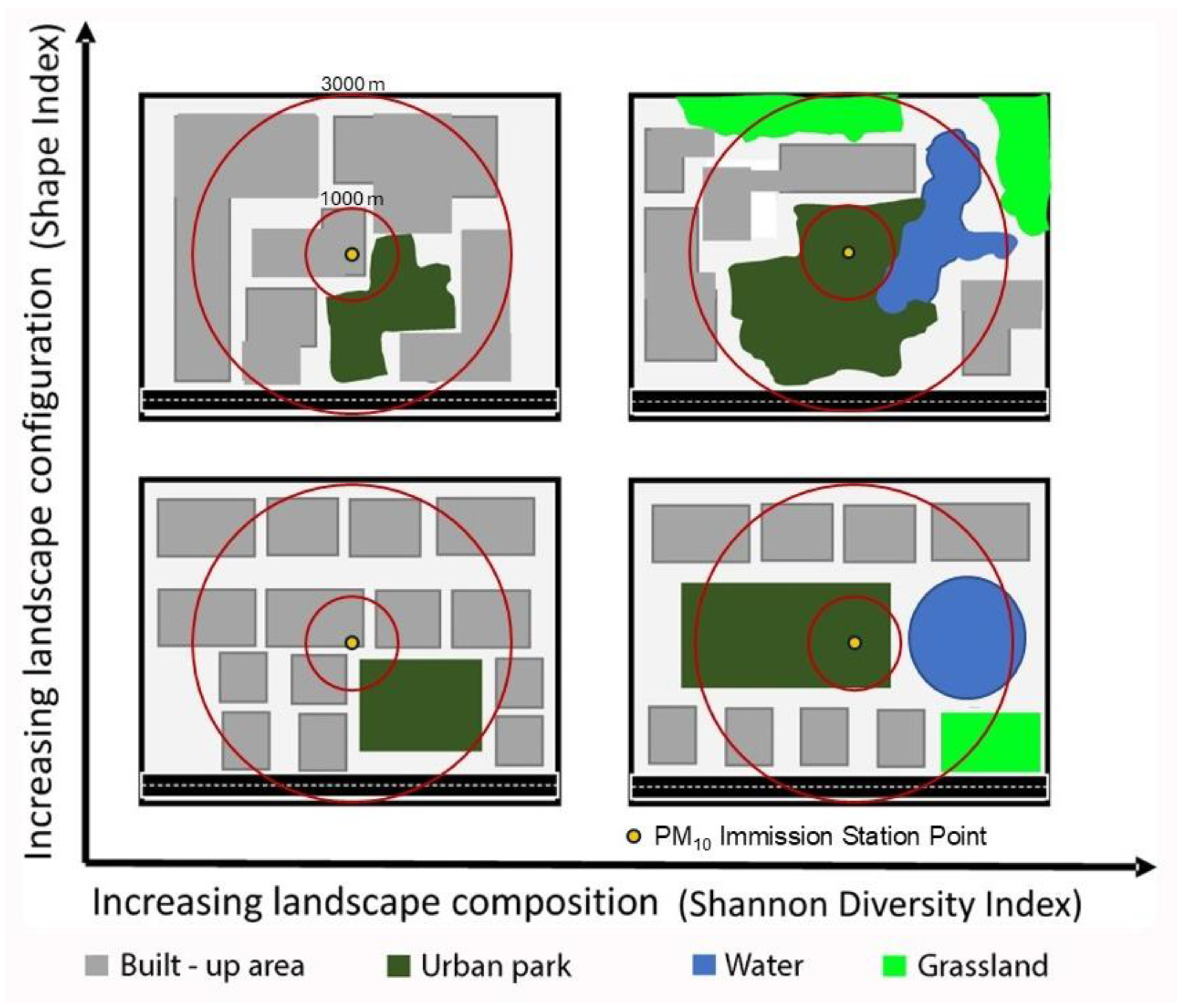
2.2.1. Calculation of Landscape Metrics
2.2.2. Calculation of Soil and Meteorological Factors
2.3. Statistical Analyzes
2.3.1. Random Forest Modeling (RF)
2.3.2. Model Development
2.3.3. Model Evaluation
2.3.4. Feature Importance
2.3.5. Spearman Coefficient Correlation
3. Results
3.1. Improvements to the Model’s Performance
3.2. Analysis of Independent Variable Importance and Spearman Correlation Coefficient
3.2.1. Heating Period
3.2.2. Cooling Period
3.2.3. Effect of Different Soil Texture Categories
4. Discussion
4.1. Model Improvement
4.2. Effects of Climatological Variables
4.3. Effects of Landscape Metrics
4.4. Effect of Different Soil Textures
5. Conclusions
Author Contributions
Funding
Data Availability Statement
Conflicts of Interest
Appendix A

| Buffer Zone | Period | RMSE Test Set (30%) Previous Study CRF Modeling | MAE Test Set (30%) Previous Study CRF Modeling | RMSE Test Set (30%) RF Modeling | MAE Test Set (30%) RF Modeling |
|---|---|---|---|---|---|
| 1000 m | Cooling | 4.84 | 3.58 | 3.72 | 2.74 |
| 3000 m | Cooling | 4.63 | 3.35 | 4.02 | 2.95 |
| 1000 m | Heating | 6.83 | 4.92 | 5.97 | 4.29 |
| 3000 m | Heating | 6.64 | 4.70 | 5.96 | 4.18 |
| Independent Variable | VIF | |||
|---|---|---|---|---|
| Cooling Period | Heating Period | |||
| 1000 m | 3000 m | 1000 m | 3000 m | |
| MPS of PM10 Source LULC Categories | 1.911885 | 3.028666 | 1.962884 | 3.302535 |
| MPS of PM10 Barriers | 4.480291 | 2.597356 | 4.250656 | 3.024115 |
| MPS of LULC Categories with Changeable Effect on PM10 | 2.393220 | 1.234664 | 2.180816 | 1.229374 |
| SHI of PM10 Source LULC Categories | 1.250877 | 2.586977 | 1.197091 | 2.005047 |
| SHI of PM10 Barriers | 1.662593 | 1.385610 | 1.600599 | 1.365938 |
| SHI of LULC with Changeable Effect on PM10 | 1.867300 | 1.215057 | 1.828440 | 1.243012 |
| SHDI | 1.991132 | 1.754137 | 1.990479 | 1.598674 |
| CI1 | 4.958673 | 3.818949 | 5.124483 | 4.751261 |
| CI2 | 7.327620 | 8.215971 | 8.187491 | 8.902750 |
| CCE | 8.344573 | 8.360450 | 7.445902 | 8.745668 |
| Air Pressure | 1.264055 | 1.281203 | 1.070224 | 1.095389 |
| Total Precipitation | 1.370848 | 1.500650 | 1.174197 | 1.181026 |
| Temperature | 1.417126 | 1.416542 | 1.123252 | 1.149163 |
| Wind Speed | 1.210010 | 1.430629 | 1.101249 | 1.259422 |
| PLAND of Built-Up Area | 8.380624 | 5.520451 | 8.361314 | 6.866883 |
| PLAND of Industrial Unit | 7.301525 | 2.820040 | 8.230368 | 3.356350 |
| PLAND of Roads | 4.815526 | 3.281017 | 3.957730 | 3.625052 |
| PLAND of Railways | 2.701912 | 1.511417 | 2.355532 | 1.600790 |
| PLAND of Mine, Dump, and Construction Sites | 1.139129 | 1.331924 | 1.174259 | 1.340900 |
| PLAND of Vacant Lands | 1.473016 | 1.254967 | 1.335742 | 1.277378 |
| PLAND of Urban Parks | 8.808699 | 2.836596 | 6.219159 | 3.207821 |
| PLAND of Arable Lands | 8.375765 | 6.910781 | 4.691872 | 7.744227 |
| PLAND of Grasslands | 6.632918 | 3.712766 | 4.380273 | 4.683871 |
| PLAND of Forests | 6.945185 | 3.460085 | 6.028392 | 4.489963 |
| PLAND of Water | 2.848026 | 2.002094 | 2.481236 | 2.822331 |
References
- Kuerban, M.; Waili, Y.; Fan, F.; Liu, Y.; Qin, W.; Dore, A.J.; Peng, J.; Xu, W.; Zhang, F. Spatio-Temporal Patterns of Air Pollution in China from 2015 to 2018 and Implications for Health Risks. Environ. Pollut. 2020, 258, 113659. [Google Scholar] [CrossRef] [PubMed]
- Zhang, Z.; Wu, L.; Chen, Y. Forecasting PM2.5 and PM10 Concentrations Using GMCN(1,N) Model with the Similar Meteorological Condition: Case of Shijiazhuang in China. Ecol. Indic. 2020, 119, 106871. [Google Scholar] [CrossRef]
- Žibert, J.; Cedilnik, J.; Pražnikar, J. Particulate Matter (PM10) Patterns in Europe: An Exploratory Data Analysis Using Non-Negative Matrix Factorization. Atmos. Environ. 2016, 132, 217–228. [Google Scholar] [CrossRef]
- Subramanian, A.; Khatri, S.B. The Exposome and Asthma. Clin. Chest Med. 2019, 40, 107–123. [Google Scholar] [CrossRef] [PubMed]
- Beloconi, A.; Vounatsou, P. Revised EU and WHO Air Quality Thresholds: Where Does Europe Stand? Atmos. Environ. 2023, 314, 120110. [Google Scholar] [CrossRef]
- European Parliament and Council of the European Union. Directive 2008/50/EC of the European Parliament and of the Council. Off. J. Eur. Union 2008, 133, 19–40. [Google Scholar]
- European Parliament. Council of the European Union DIRECTIVE (EU) 2024/2881 on Ambient Air Quality and Cleaner Air for Europe. Off. J. Eur. Union 2024, 2881, 1–70. [Google Scholar]
- Guerreiro, C.B.B.; Foltescu, V.; de Leeuw, F. Air Quality Status and Trends in Europe. Atmos. Environ. 2014, 98, 376–384. [Google Scholar] [CrossRef]
- Vardoulakis, S.; Kassomenos, P. Sources and Factors Affecting PM 10 Levels in Two European Cities: Implications for Local Air Quality Management. Atmos. Environ. 2008, 42, 3949–3963. [Google Scholar] [CrossRef]
- Uuemaa, E.; Mander, Ü.; Marja, R. Trends in the Use of Landscape Spatial Metrics as Landscape Indicators: A Review. Ecol. Indic. 2013, 28, 100–106. [Google Scholar] [CrossRef]
- Uuemaa, E.; Antrop, M.; Roosaare, J.; Marja, R.; Mander, Ü. Landscape Metrics and Indices: An Overview of Their Use in Landscape Research. Living Rev. Landsc. Res. 2009, 3, 1–28. [Google Scholar] [CrossRef]
- Sohrab, S.; Csikós, N.; Szilassi, P. Effect of Geographical Parameters on PM10 Pollution in European Landscapes: A Machine Learning Algorithm-Based Analysis. Environ. Sci. Eur. 2024, 36, 152. [Google Scholar] [CrossRef]
- Robinson, H.S.; Weckworth, B. Landscape Ecology: Linking Landscape Metrics to Ecological Processes. In Snow Leopards: Biodiversity of the World: Conservation from Genes to Landscapes; Academic Press: Cambridge, MA, USA, 2016; pp. 395–405. [Google Scholar] [CrossRef]
- Forman, R.T.T. Some General Principles of Landscape and Regional Ecology. Landsc. Ecol. 1995, 10, 133–142. [Google Scholar] [CrossRef]
- Herzog, H.; Caldeira, K.; Reilly, J. An Issue of Permanence: Assessing the Effectiveness of Temporary Carbon Storage. Clim. Chang. 2003, 59, 293–310. [Google Scholar] [CrossRef]
- Haberl, H.; Wackernagel, M.; Wrbka, T. Land Use and Sustainability Indicators. An Introduction. Land Use Policy 2004, 21, 193–198. [Google Scholar] [CrossRef]
- Tasser, E.; Sternbach, E.; Tappeiner, U. Biodiversity Indicators for Sustainability Monitoring at Municipality Level: An Example of Implementation in an Alpine Region. Ecol. Indic. 2008, 8, 204–223. [Google Scholar] [CrossRef]
- Renetzeder, C.; Schindler, S.; Peterseil, J.; Prinz, M.A.; Mücher, S.; Wrbka, T. Can We Measure Ecological Sustainability? Landscape Pattern as an Indicator for Naturalness and Land Use Intensity at Regional, National and European Level. Ecol. Indic. 2010, 10, 39–48. [Google Scholar] [CrossRef]
- Schindler, S.; Sebesvari, Z.; Damm, C.; Euller, K.; Mauerhofer, V.; Schneidergruber, A.; Biró, M.; Essl, F.; Kanka, R.; Lauwaars, S.G.; et al. Multifunctionality of Floodplain Landscapes: Relating Management Options to Ecosystem Services. Landsc. Ecol. 2014, 29, 229–244. [Google Scholar] [CrossRef]
- Lausch, A.; Blaschke, T.; Haase, D.; Herzog, F.; Syrbe, R.U.; Tischendorf, L.; Walz, U. Understanding and Quantifying Landscape Structure—A Review on Relevant Process Characteristics, Data Models and Landscape Metrics. Ecol. Model. 2015, 295, 31–41. [Google Scholar] [CrossRef]
- Szilassi, P.; Bata, T.; Szabó, S.; Czúcz, B.; Molnár, Z.; Mezősi, G. The Link between Landscape Pattern and Vegetation Naturalness on a Regional Scale. Ecol. Indic. 2017, 81, 252–259. [Google Scholar] [CrossRef]
- Gál, T.; Skarbit, N.; Unger, J. Urban Heat Island Patterns and Their Dynamics Based on an Urban Climate Measurement Network. Hung. Geogr. Bull. 2016, 65, 105–116. [Google Scholar] [CrossRef]
- Gallé, R.; Happe, A.K.; Baillod, A.B.; Tscharntke, T.; Batáry, P. Landscape Configuration, Organic Management, and within-Field Position Drive Functional Diversity of Spiders and Carabids. J. Appl. Ecol. 2019, 56, 63–72. [Google Scholar] [CrossRef]
- Jeanneret, P.; Aviron, S.; Alignier, A.; Lavigne, C.; Helfenstein, J.; Herzog, F.; Kay, S.; Petit, S. Agroecology Landscapes. Landsc. Ecol. 2021, 36, 2235–2257. [Google Scholar] [CrossRef]
- Lin, F.; Chen, X. Effects of Landscape Patterns on Atmospheric Particulate Matter Concentrations in Fujian Province, China. Atmosphere 2023, 14, 787. [Google Scholar] [CrossRef]
- Ku, C.A. Exploring the Spatial and Temporal Relationship between Air Quality and Urban Land-Use Patterns Based on an Integrated Method. Sustainability 2020, 12, 2964. [Google Scholar] [CrossRef]
- Zhang, J.; Wang, X.; Xie, Y. Implication of Buffer Zones Delineation Considering the Landscape Connectivity and Influencing Patch Structural Factors in Nature Reserves. Sustainability 2021, 13, 10833. [Google Scholar] [CrossRef]
- Jaafari, S.; Shabani, A.A.; Moeinaddini, M.; Danehkar, A.; Sakieh, Y. Applying Landscape Metrics and Structural Equation Modeling to Predict the Effect of Urban Green Space on Air Pollution and Respiratory Mortality in Tehran. Environ. Monit. Assess. 2020, 192, 412. [Google Scholar] [CrossRef] [PubMed]
- Łowicki, D. Landscape Pattern as an Indicator of Urban Air Pollution of Particulate Matter in Poland. Ecol. Indic. 2019, 97, 17–24. [Google Scholar] [CrossRef]
- Li, F.; Zhou, T.; Lan, F. Relationships between Urban Form and Air Quality at Different Spatial Scales: A Case Study from Northern China. Ecol. Indic. 2021, 121, 107029. [Google Scholar] [CrossRef]
- Xu, W.; Jin, X.; Liu, M.; Ma, Z.; Wang, Q.; Zhou, Y. Analysis of Spatiotemporal Variation of PM2.5 and Its Relationship to Land Use in China. Atmos. Pollut. Res. 2021, 12, 101151. [Google Scholar] [CrossRef]
- Park, Y.; Shin, J.; Lee, J.Y. Spatial Association of Urban Form and Particulate Matter. Int. J. Environ. Res. Public Health 2021, 18, 9428. [Google Scholar] [CrossRef] [PubMed]
- McGarigal, K.; Marks, B.J. FRAGSTATS: Spatial Pattern Analysis Program for Quantifying Landscape Structure; US Department of Agriculture, Forest Service, Pacific Northwest Research Station: Dolores, CO, USA, 1995; 122p. [CrossRef]
- Hu, H.; Zeng, S.; Han, X. Effects of Urban Landscapes on Pollutant Concentrations in Chengdu Plain Urban Agglomeration. Atmosphere 2022, 13, 1492. [Google Scholar] [CrossRef]
- Zeng, C.; Song, Y.; He, Q.; Liu, Y. Urban–Rural Income Change: Influences of Landscape Pattern and Administrative Spatial Spillover Effect. Appl. Geogr. 2018, 97, 248–262. [Google Scholar] [CrossRef]
- Sterzyńska, M.; Nicia, P.; Zadrożny, P.; Fiera, C.; Shrubovych, J.; Ulrich, W. Urban Springtail Species Richness Decreases with Increasing Air Pollution. Ecol. Indic. 2018, 94, 328–335. [Google Scholar] [CrossRef]
- Sohrab, S.; Csikos, N.; Szilassi, P. Effects of Land Use Patterns on PM10 Concentrations in Urban and Suburban Areas. A European Scale Analysis. Atmos. Pollut. Res. 2023, 14, 101942. [Google Scholar] [CrossRef]
- Lublin, P.M.; Kujawska, J.; Kulisz, M.; Oleszczuk, P.; Cel, W. Machine Learning Methods to Forecast the Concentration of PM10 in Lublin, Poland. Energies 2022, 15, 6428. [Google Scholar] [CrossRef]
- Guo, Q.; He, Z.; Wang, Z. Prediction of Hourly PM2.5 and PM10 Concentrations in Chongqing City in China Based on Artificial Neural Network. Aerosol. Air Qual. Res. 2023, 23, 220448. [Google Scholar] [CrossRef]
- Shaziayani, W.N.; Ul-Saufie, A.Z.; Mutalib, S.; Mohamad Noor, N.; Zainordin, N.S. Classification Prediction of PM10 Concentration Using a Tree-Based Machine Learning Approach. Atmosphere 2022, 13, 538. [Google Scholar] [CrossRef]
- Mampitiya, L.; Rathnayake, N.; Hoshino, Y.; Rathnayake, U. Performance of Machine Learning Models to Forecast PM10 Levels. MethodsX 2024, 12, 102557. [Google Scholar] [CrossRef]
- Jemeļjanova, M.; Kmoch, A.; Uuemaa, E. Adapting Machine Learning for Environmental Spatial Data—A Review. Ecol. Inform. 2024, 81, 102634. [Google Scholar] [CrossRef]
- Farmonov, N.; Amankulova, K.; Khan, S.N.; Abdurakhimova, M.; Szatmári, J.; Khabiba, T.; Makhliyo, R.; Khodicha, M.; Mucsi, L. Effectiveness of Machine Learning and Deep Learning Models at County-Level Soybean Yield Forecasting. Hung. Geogr. Bull. 2023, 72, 383–398. [Google Scholar] [CrossRef]
- Breiman, L. Random Forests. Mach. Learn. 2001, 45, 5–32. [Google Scholar] [CrossRef]
- Hartmann, P.; Urso, L.; Petermann, E.; Gn, F. Use of Random Forest Algorithm for Predictive Modelling of Transfer Factor Soil-Plant for Radiocaesium: A Feasibility Study. J. Environ. Radioact. 2023, 270, 107309. [Google Scholar] [CrossRef]
- Simon, S.M.; Glaum, P.; Valdovinos, F.S. Interpreting Random Forest Analysis of Ecological Models to Move from Prediction to Explanation. Sci. Rep. 2023, 13, 3881. [Google Scholar] [CrossRef]
- Brugere, L.; Kwon, Y.; Frazier, A.E.; Kedron, P. Forest Ecology and Management Improved Prediction of Tree Species Richness and Interpretability of Environmental Drivers Using a Machine Learning Approach. For. Ecol. Manag. 2023, 539, 120972. [Google Scholar] [CrossRef]
- Cappelli, F.; Castronuovo, G.; Grimaldi, S. Random Forest and Feature Importance Measures for Discriminating the Most Influential Environmental Factors in Predicting Cardiovascular and Respiratory Diseases. Int. J. Environ. Res. Public Health 2024, 21, 867. [Google Scholar] [CrossRef]
- Czernecki, B.; Marosz, M.; Jędruszkiewicz, J. Assessment of Machine Learning Algorithms in Short-Term Forecasting of PM10 and PM2.5 Concentrations in Selected Polish Agglomerations. Aerosol Air Qual. Res. 2016, 21, 1–18. [Google Scholar] [CrossRef]
- Ricardo, A.; Valencia, Z.; Alfonso, A.; Rosales, R. Application of Random Forest in a Predictive Model of PM10 Particles in Mexico City. Nat. Environ. Pollut. Technol. 2024, 23, 711–724. [Google Scholar] [CrossRef]
- Mamić, L.; Gašparović, M. Developing PM2.5 and PM10 Prediction Models on a National and Regional Scale Using Open-Source Remote Sensing Data. Environ. Monit. Assess. 2023, 195, 644. [Google Scholar] [CrossRef]
- European Environment Agency (EEA). The European Air Quality (AQ) Portal. Available online: https://www.eea.europa.eu/en/analysis/maps-and-charts/ (accessed on 12 October 2022).
- EEA Urban Atlas 2018. Available online: https://land.copernicus.eu/local/urban-atlas/urban-atlas-2018 (accessed on 26 January 2023).
- Panagos, P.; Van Liedekerke, M.; Borrelli, P.; Köninger, J.; Ballabio, C.; Orgiazzi, A.; Lugato, E.; Liakos, L.; Hervas, J.; Jones, A.; et al. European Soil Data Centre 2.0: Soil Data and Knowledge in Support of the EU Policies. Eur. J. Soil Sci. 2022, 73, e13315. [Google Scholar] [CrossRef]
- Hersbach, H.; Bell, B.; Berrisford, P.; Biavati, G.; Horányi, A.; Muñoz Sabater, J.; Nicolas, J.; Peubey, C.; Radu, R.; Rozum, I.; et al. ERA5 Monthly Averaged Data on Single Levels from 1940 to Present. Available online: https://cds.climate.copernicus.eu/cdsapp?fbclid=IwAR1BDSE0WQUyGWYaB2wsTw2DsRLRlsQz4dnuNy0wcS1tmM65sQP_EkeKPWk#!/dataset/reanalysis-era5-single-levels-monthly-means?tab=form (accessed on 30 November 2023).
- Liu, Y.; Wu, J.; Yu, D. Characterizing Spatiotemporal Patterns of Air Pollution in China: A Multiscale Landscape Approach. Ecol. Indic. 2017, 76, 344–356. [Google Scholar] [CrossRef]
- Sohrab, S.; Csikós, N.; Szilassi, P. Connection between the Spatial Characteristics of the Road and Railway Networks and the Air Pollution (PM10) in Urban–Rural Fringe Zones. Sustainability 2022, 14, 10103. [Google Scholar] [CrossRef]
- World Health Organization. WHO Housing and Health Guidelines; WHO: Geneva, Switzerland, 2018; ISBN 9789241550376. [Google Scholar]
- Moreci, E.; Ciulla, G.; Lo Brano, V. Annual Heating Energy Requirements of Office Buildings in a European Climate. Sustain. Cities Soc. 2016, 20, 81–95. [Google Scholar] [CrossRef]
- Jin, Z.; Zheng, Y.; Zhang, Y. A Novel Method for Building Air Conditioning Energy Saving Potential Pre-Estimation Based on Thermodynamic Perfection Index for Space Cooling. J. Asian Archit. Build. Eng. 2023, 22, 2348–2364. [Google Scholar] [CrossRef]
- Xiong, J.; Chen, L.; Zhang, Y. Building Energy Saving for Indoor Cooling and Heating: Mechanism and Comparison on Temperature Difference. Sustainability 2023, 15, 11241. [Google Scholar] [CrossRef]
- Moustris, K.P.; Zacharia, P.T.; Larissi, I.K.; Nastos, P.T.; Paliatsos, A.G. Cooling and Heating Degree-Days Calculation for Representative Locations Within the Greater Athens Area, Greece. In Proceedings of the 12th International Conference on Environmental Science and Technology, Rhodes, Greece, 8–10 October 2011; pp. 8–10. [Google Scholar]
- Cutler, D.R.; Edwards, T.C.; Beard, K.H.; Cutler, A.; Hess, K.T.; Gibson, J.; Lawler, J.J. Random Forests for Classification in Ecology. Ecology 2007, 88, 2783–2792. [Google Scholar] [CrossRef]
- Kohavi, R. A Study of Cross-Validation and Bootstrap for Accuracy Estimation and Model Selection. IJCAI Int. Jt. Conf. Artif. Intell. 1995, 2, 1137–1143. [Google Scholar]
- Zaharia, M.; Xin, R.S.; Wendell, P.; Das, T.; Armbrust, M.; Dave, A.; Meng, X.; Rosen, J.; Venkataraman, S.; Franklin, M.J.; et al. Apache Spark: A Unified Engine for Big Data Processing. Commun. ACM 2016, 59, 56–65. [Google Scholar] [CrossRef]
- Pedregosa, F.; Varoquaux, G.; Gramfort, A.; Michel, V.; Thirion, B.; Grisel, O.; Blondel, M.; Prettenhofer, P.; Weiss, R.; Dubourg, V.; et al. Scikit-Learn: Machine Learning in Python. J. Mach. Learn. Res. 2011, 12, 2825–2830. [Google Scholar]
- Buitinck, L.; Louppe, G.; Blondel, M.; Pedregosa, F.; Mueller, A.; Grisel, O.; Niculae, V.; Prettenhofer, P.; Gramfort, A.; Grobler, J.; et al. API Design for Machine Learning Software: Experiences from the Scikit-Learn Project. arXiv 2013, arXiv:1309.0238. [Google Scholar]
- Varoquaux, G.; Buitinck, L.; Louppe, G.; Grisel, O.; Pedregosa, F.; Mueller, A. Scikit-Learn. GetMobile Mob. Comput. Commun. 2015, 19, 29–33. [Google Scholar] [CrossRef]
- Evans, J.S.; Murphy, M.A.; Holden, Z.A. Modeling Species Distribution and Change Using Random Forest. In Predictive Species and Habitat Modeling in Landscape Ecology; Springer: New York, NY, USA, 2011; Chapter 8. [Google Scholar] [CrossRef]
- Hastie, T.; Tibshirani, R.; Friedman, J. The Elements of Statistical Learning Data Mining, Inference, and Prediction, 2nd ed.; Springer: Berlin/Heidelberg, Germany, 2009; ISBN 9781479932115. [Google Scholar]
- Res, C.; Willmott, C.J.; Matsuura, K. Advantages of the Mean Absolute Error (MAE) over the Root Mean Square Error (RMSE) in Assessing Average Model Performance. Clim. Res. 2005, 30, 79–82. [Google Scholar]
- Chai, T.; Draxler, R.R. Root Mean Square Error (RMSE) or Mean Absolute Error (MAE)? -Arguments against Avoiding RMSE in the Literature. Geosci. Model. Dev. 2014, 7, 1247–1250. [Google Scholar] [CrossRef]
- Karunasingha, D.S.K. Root Mean Square Error or Mean Absolute Error? Use Their Ratio as Well. Inf. Sci. 2022, 585, 609–629. [Google Scholar] [CrossRef]
- Barmpadimos, I.; Hueglin, C.; Keller, J.; Henne, S.; Prévôt, A.S.H. Influence of Meteorology on PM10 Trends and Variability in Switzerland from 1991 to 2008. Atmos. Chem. Phys. 2011, 11, 1813–1835. [Google Scholar] [CrossRef]
- Peng, L.; Zhao, X.; Tao, Y.; Mi, S.; Huang, J.; Zhang, Q. The Effects of Air Pollution and Meteorological Factors on Measles Cases in Lanzhou, China. Environ. Sci. Pollut. Res. 2020, 27, 13524–13533. [Google Scholar] [CrossRef] [PubMed]
- Birinci, E.; Deniz, A.; Özdemir, E.T. The Relationship between PM10 and Meteorological Variables in the Mega City Istanbul. Environ. Monit. Assess. 2023, 195, 304. [Google Scholar] [CrossRef]
- Galindo, N.; Varea, M.; Gil-Moltó, J.; Yubero, E.; Nicolás, J. The Influence of Meteorology on Particulate Matter Concentrations at an Urban Mediterranean Location. Water. Air. Soil Pollut. 2011, 215, 365–372. [Google Scholar] [CrossRef]
- Li, Y.; Chen, Q.; Zhao, H.; Wang, L.; Tao, R. Variations in Pm10, Pm2.5 and Pm1.0 in an Urban Area of the Sichuan Basin and Their Relation to Meteorological Factors. Atmosphere 2015, 6, 150–163. [Google Scholar] [CrossRef]
- Birim, N.G.; Turhan, C.; Atalay, A.S.; Gokcen Akkurt, G. The Influence of Meteorological Parameters on PM10: A Statistical Analysis of an Urban and Rural Environment in Izmir/Türkiye. Atmosphere 2023, 14, 421. [Google Scholar] [CrossRef]
- Dung, N.A.; Son, D.H.; Hanh, N.T.D.; Tri, D.Q. Effect of Meteorological Factors on PM10 Concentration in Hanoi, Vietnam. J. Geosci. Environ. Prot. 2019, 7, 138–150. [Google Scholar] [CrossRef]
- Giri, D.; Krishna Murthy, V.; Adhikary, P.R. The influence of meteorological conditions on PM10 concentrations in Kathmandu Valley. Int. J. Environ. Res. 2008, 2, 49–60. [Google Scholar]
- Özdemir, U.; Taner, S. Impacts of Meteorological Factors on PM10: Artificial Neural Networks (ANN) and Multiple Linear Regression (MLR) Approaches. Environ. Forensics 2014, 15, 329–336. [Google Scholar] [CrossRef]
- Talepour, N.; Birgani, Y.T.; Kelly, F.J.; Jaafarzadeh, N.; Goudarzi, G. Analyzing Meteorological Factors for Forecasting PM10 and PM2.5 Levels: A Comparison between MLR and MLP Models. Earth Sci. Inform. 2024, 17, 5603–5623. [Google Scholar] [CrossRef]
- Tian, Y.; Yao, X. Urban Form, Traffic Volume, and Air Quality: A Spatiotemporal Stratified Approach. Environ. Plan. B Urban Anal. City Sci. 2021, 49, 92–113. [Google Scholar] [CrossRef]
- Zeb, B.; Ditta, A.; Alam, K.; Sorooshian, A.; Din, B.U.; Iqbal, R.; Habib ur Rahman, M.; Raza, A.; Alwahibi, M.S.; Elshikh, M.S. Wintertime Investigation of PM10 Concentrations, Sources, and Relationship with Different Meteorological Parameters. Sci. Rep. 2024, 14, 154. [Google Scholar] [CrossRef] [PubMed]
- Volná, V.; Hladkỳ, D. Detailed Assessment of the Effects of Meteorological Conditions on PM10 Concentrations in the Northeastern Part of the Czech Republic. Atmosphere 2020, 11, 497. [Google Scholar] [CrossRef]
- Mok, K.M.; Hoi, K.I. Effects of Meteorological Conditions on PM10 Concentrations—A Study in Macau. Environ. Monit. Assess. 2005, 102, 201–223. [Google Scholar] [CrossRef]
- Tian, G.; Qiao, Z.; Xu, X. Characteristics of Particulate Matter (PM10) and Its Relationship with Meteorological Factors during 2001–2012 in Beijing. Environ. Pollut. 2014, 192, 266–274. [Google Scholar] [CrossRef] [PubMed]
- Wu, J.; Xie, W.; Li, W.; Li, J. Effects of Urban Landscape Pattern on PM2.5 Pollution-A Beijing Case Study. PLoS ONE 2015, 10, e0142449. [Google Scholar] [CrossRef] [PubMed]
- Ai, H.; Zhang, X.; Zhou, Z. The Impact of Greenspace on Air Pollution: Empirical Evidence from China. Ecol. Indic. 2023, 146, 109881. [Google Scholar] [CrossRef]
- Jiang, R.; Xie, C.; Man, Z.; Zhou, R.; Che, S. Effects of Urban Green and Blue Space on the Diffusion Range of PM2.5 and PM10 Based on LCZ. Land 2023, 12, 964. [Google Scholar] [CrossRef]
- Yoon, S.; Heo, Y.; Park, C.; Kang, W. Effects of Landscape Patterns on the Concentration and Recovery Time of PM2.5 in South Korea. Land 2022, 11, 2176. [Google Scholar] [CrossRef]
- Yang, D.; Meng, F.; Liu, Y.; Dong, G.; Lu, D. Scale Effects and Regional Disparities of Land Use in Influencing PM2.5 Concentrations: A Case Study in the Zhengzhou Metropolitan Area, China. Land 2022, 11, 1538. [Google Scholar] [CrossRef]
- Ren, W.; Zhao, J.; Ma, X. Analysis of the Spatial Characteristics of Inhalable Particulate Matter Concentrations under the Influence of a Three-Dimensional Landscape Pattern in Xi’an, China. Sustain. Cities Soc. 2022, 81, 103841. [Google Scholar] [CrossRef]
- Li, C.; Zhang, K.; Dai, Z.; Ma, Z.; Liu, X. Investigation of the Impact of Land-Use Distribution on Pm2.5 in Weifang: Seasonal Variations. Int. J. Environ. Res. Public Health 2020, 17, 5135. [Google Scholar] [CrossRef]
- Yang, H.; Leng, Q.; Xiao, Y.; Chen, W. Investigating the Impact of Urban Landscape Composition and Configuration on PM2.5 Concentration under the LCZ Scheme: A Case Study in Nanchang, China. Sustain. Cities Soc. 2022, 84, 104006. [Google Scholar] [CrossRef]
- Huang, D.; He, B.; Wei, L.; Sun, L.; Li, Y.; Yan, Z.; Wang, X.; Chen, Y.; Li, Q.; Feng, S. Impact of Land Cover on Air Pollution at Different Spatial Scales in the Vicinity of Metropolitan Areas. Ecol. Indic. 2021, 132, 108313. [Google Scholar] [CrossRef]
- Gkyer, E. Understanding Landscape Structure Using Landscape Metrics. In Advances in Landscape Architecture; IntechOpen: London, UK, 2013. [Google Scholar] [CrossRef]
- Kim, H.; Hong, S. Relationship between Land-Use Type and Daily Concentration and Variability of PM10 in Metropolitan Cities: Evidence from South Korea. Land 2022, 11, 23. [Google Scholar] [CrossRef]
- Yu, Y.; Cao, J. Chemical Fingerprints and Source Profiles of PM10 and PM2.5 from Agricultural Soil in a Typical Polluted Region of Northwest China. Aerosol Air Qual. Res. 2023, 23, 220419. [Google Scholar] [CrossRef]
- Aimar, S.B.; Mendez, M.J.; Funk, R.; Buschiazzo, D.E. Soil Properties Related to Potential Particulate Matter Emissions (PM10) of Sandy Soils. Aeolian Res. 2012, 3, 437–443. [Google Scholar] [CrossRef]
- Zobeck, T.M.; Amante-Orozco, A. Effect of Dust Source Clay and Carbonate Content on Fugitive Dust Emissions. In Proceedings of the 10th International Emission Inventory Conference—“One Atmosphere, One Inventory, Many Challenges”, Denver, CO, USA, 1–3 May 2001; pp. 1–13. [Google Scholar]
- Carvacho, O.F.; Ashbaugh, L.L.; Brown, M.S.; Flocchini, R.G. Measurement of PM2.5 Emission Potential from Soil Using the UC Davis Resuspension Test Chamber. Geomorphology 2004, 59, 75–80. [Google Scholar] [CrossRef]
- Carvacho, O.F.; Ashbaugh, L.L.; Brown, M.S.; Flocchini, R.G. Relationship between San Joaquin Valley Soil Texture and PM10 Emission Potential Using the UC Davis Dust Resuspension Test Chamber. Trans. Am. Soc. Agric. Eng. 2001, 44, 1603–1608. [Google Scholar] [CrossRef]
- Péterfalvi, N.; Keller, B.; Magyar, M. PM10 Emission from Crop Production and Agricultural Soils. Agrokem. Talajt. 2018, 67, 143–159. [Google Scholar] [CrossRef]
- Gherboudj, I.; Beegum, S.N.; Marticorena, B.; Ghedira, H. Journal of Geophysical Research. Nature 1955, 175, 238. [Google Scholar] [CrossRef]
- Vos, H.C.; Fister, W.; von Holdt, J.R.; Eckardt, F.D.; Palmer, A.R.; Kuhn, N.J. Assessing the PM10 Emission Potential of Sandy, Dryland Soils in South Africa Using the PI-SWERL. Aeolian Res. 2021, 53, 100747. [Google Scholar] [CrossRef]
- Kim, H. Land Use Impacts on Particulate Matter Levels in Seoul, South Korea: Comparing High and Low Seasons. Land 2020, 9, 142. [Google Scholar] [CrossRef]
- Huang, Y.; Lei, C.; Liu, C.H.; Perez, P.; Forehead, H.; Kong, S.; Zhou, J.L. A Review of Strategies for Mitigating Roadside Air Pollution in Urban Street Canyons. Environ. Pollut. 2021, 280, 116971. [Google Scholar] [CrossRef] [PubMed]
- Li, S.; Zou, B.; Ma, X.; Liu, N.; Zhang, Z.; Xie, M.; Zhi, L. Improving Air Quality through Urban Form Optimization: A Review Study. Build. Environ. 2023, 243, 110685. [Google Scholar] [CrossRef]
- Choi, W.; Ranasinghe, D.; Bunavage, K.; DeShazo, J.R.; Wu, L.; Seguel, R.; Winer, A.M.; Paulson, S.E. The Effects of the Built Environment, Traffic Patterns, and Micrometeorology on Street Level Ultrafine Particle Concentrations at a Block Scale: Results from Multiple Urban Sites. Sci. Total Environ. 2016, 553, 474–485. [Google Scholar] [CrossRef] [PubMed]
- Vitaliano, S.; Cascone, S.; D’Urso, P.R. Mitigating Built Environment Air Pollution by Green Systems: An In-Depth Review. Appl. Sci. 2024, 14, 6487. [Google Scholar] [CrossRef]
- Hassan, A.M.; ELMokadem, A.A.; Megahed, N.A.; Abo Eleinen, O.M. Urban Morphology as a Passive Strategy in Promoting Outdoor Air Quality. J. Build. Eng. 2020, 29, 101204. [Google Scholar] [CrossRef]
 , landscape metrics
  , land use proportions
  , and soil texture
  . * Significant at the 0.05 level. ** Significant at the 0.01 level. *** Significant at the 0.001 level.
, landscape metrics , land use proportions , and soil texture . * Significant at the 0.05 level. ** Significant at the 0.01 level. *** Significant at the 0.001 level.
. * Significant at the 0.05 level. ** Significant at the 0.01 level. *** Significant at the 0.001 level.
, landscape metrics , land use proportions , and soil texture . * Significant at the 0.05 level. ** Significant at the 0.01 level. *** Significant at the 0.001 level.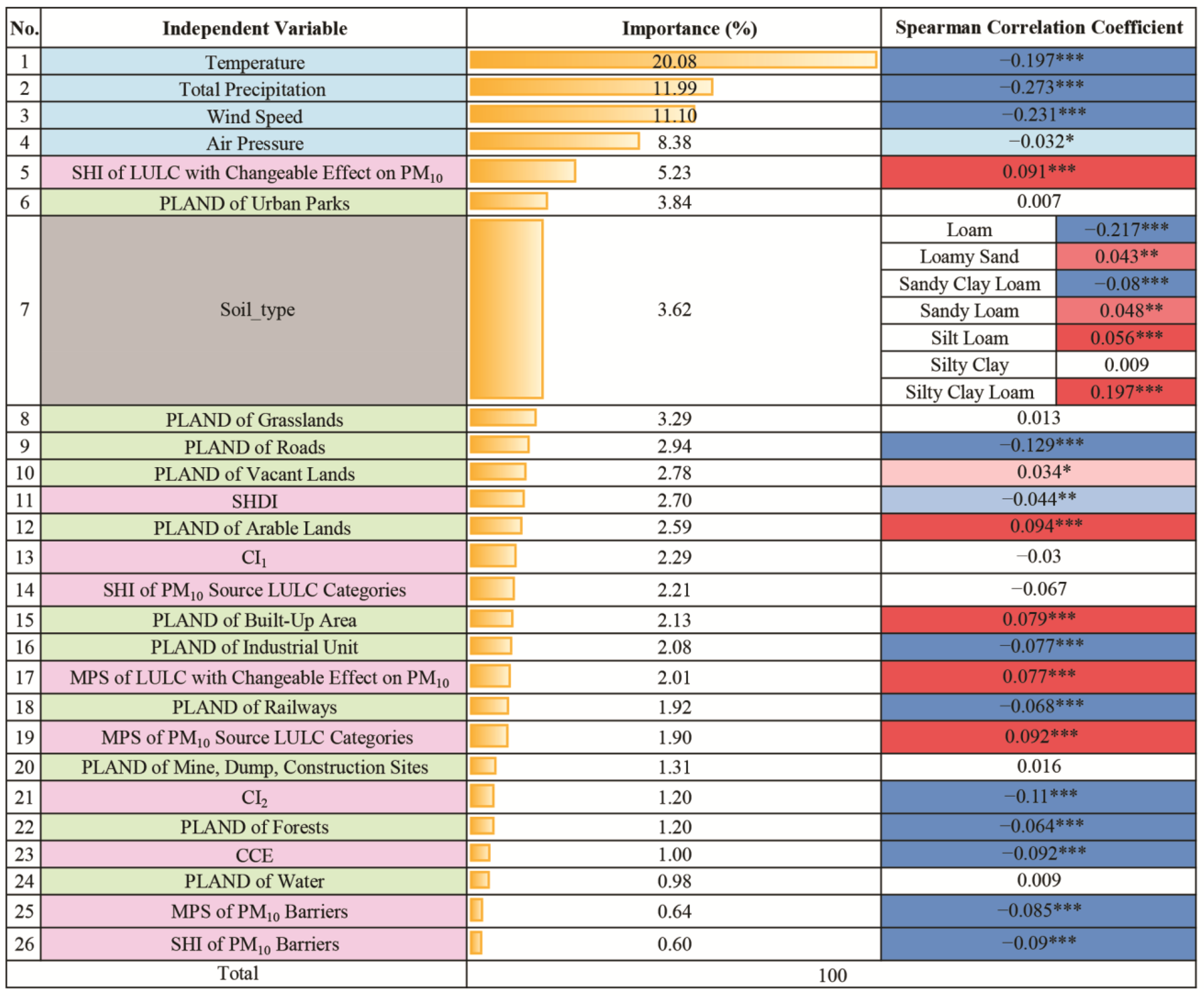
 , landscape metrics
  , land use proportions
  , and soil texture
  . ** Significant at the 0.01 level. *** Significant at the 0.001 level.
, landscape metrics , land use proportions , and soil texture . ** Significant at the 0.01 level. *** Significant at the 0.001 level.
. ** Significant at the 0.01 level. *** Significant at the 0.001 level.
, landscape metrics , land use proportions , and soil texture . ** Significant at the 0.01 level. *** Significant at the 0.001 level.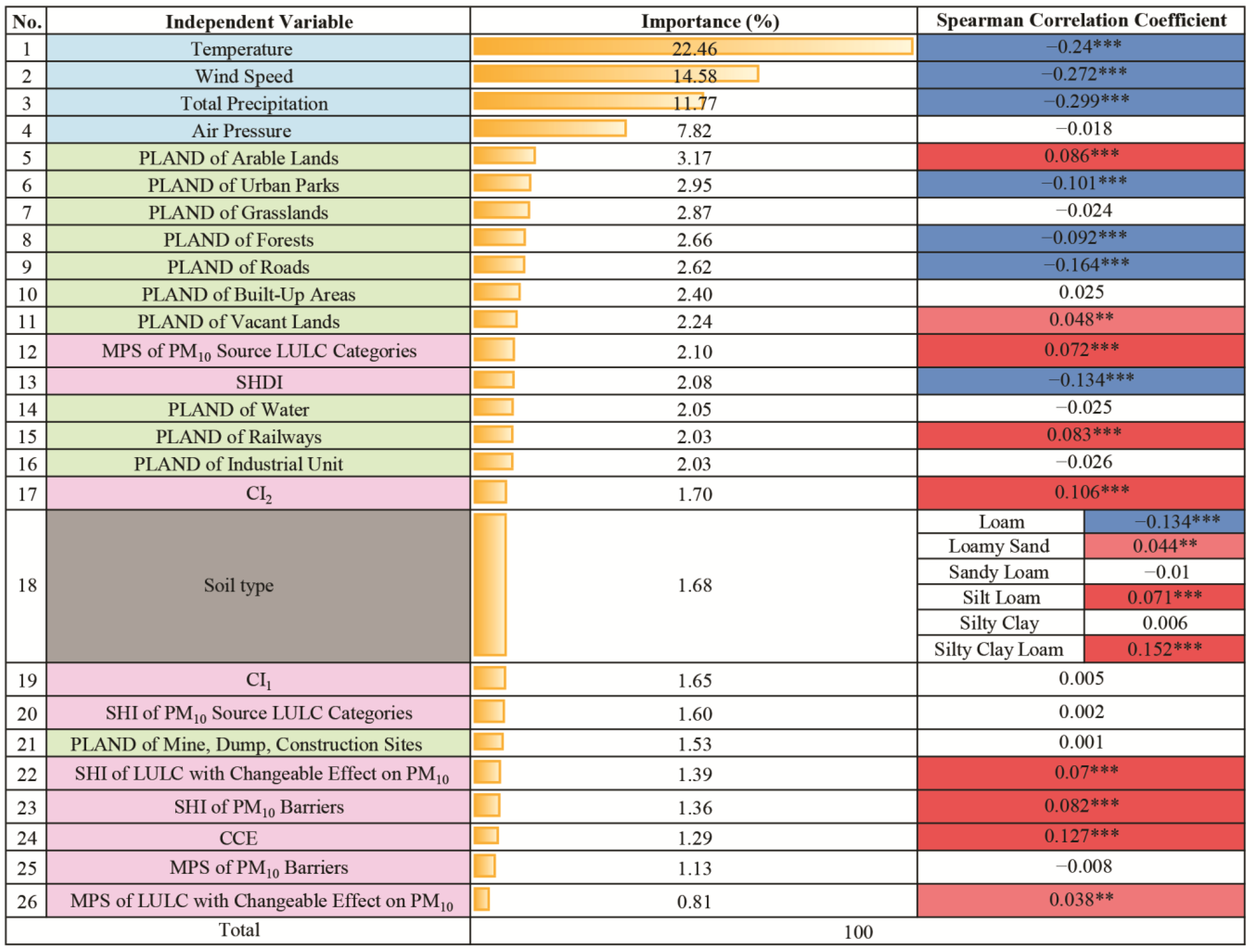
 , landscape metrics
  , land use proportions
  , and soil texture
  .* Significant at the 0.05 level. ** Significant at the 0.01 level. *** Significant at the 0.001 level.
, landscape metrics , land use proportions , and soil texture .* Significant at the 0.05 level. ** Significant at the 0.01 level. *** Significant at the 0.001 level.
.* Significant at the 0.05 level. ** Significant at the 0.01 level. *** Significant at the 0.001 level.
, landscape metrics , land use proportions , and soil texture .* Significant at the 0.05 level. ** Significant at the 0.01 level. *** Significant at the 0.001 level.
 , landscape metrics
  , land use proportions
  , and soil texture
  . * Significant at the 0.05 level. ** Significant at the 0.01 level. *** Significant at the 0.001 level.
, landscape metrics , land use proportions , and soil texture . * Significant at the 0.05 level. ** Significant at the 0.01 level. *** Significant at the 0.001 level.
. * Significant at the 0.05 level. ** Significant at the 0.01 level. *** Significant at the 0.001 level.
, landscape metrics , land use proportions , and soil texture . * Significant at the 0.05 level. ** Significant at the 0.01 level. *** Significant at the 0.001 level.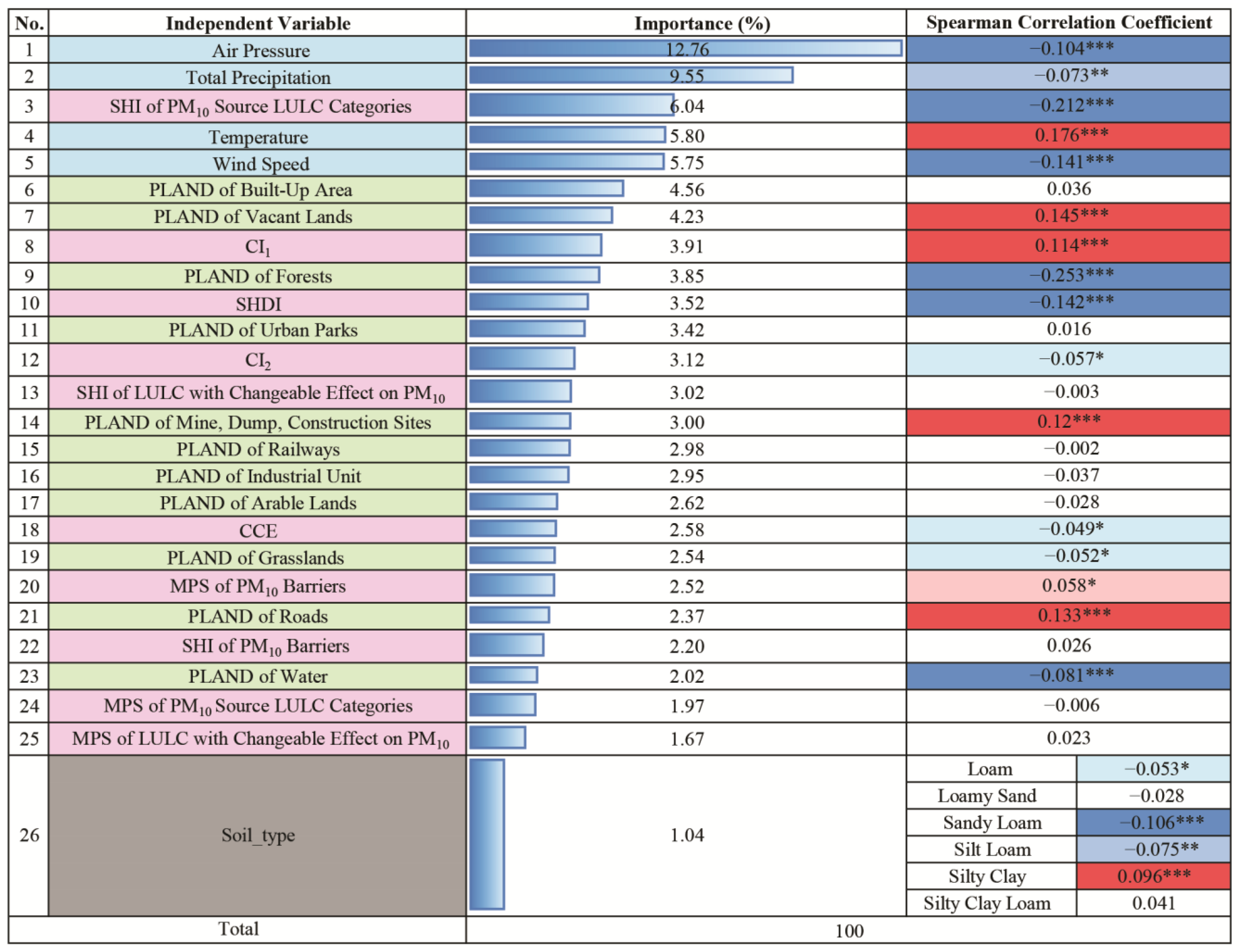
| Landscape Index | Definition |
|---|---|
| Shannon Diversity Index (SHDI) | An index based on the relative area of each landscape type and the total number of LULC types. It is more sensitive to rare patch types than Simpson’s diversity index. |
| Proportion of LULC Categories (PLANDs) | This index reflects the percentage of the total area of a certain type of LULC patch in the entire landscape area, determining the basis for judging dominant landscape elements. |
| Mean Patch Area (MPA) | The average area of patches in the landscape of each type. Calculated for each LULC group (PM10 sources, barriers, and changeable). |
| Shape Index (SHI) | Describes the complexity of the shape of LULC patches within a landscape. It compares the perimeter of a patch with the perimeter of a standard shape (usually a square or circle) with the same area, thus giving insight into how irregular or fragmented a patch is. Calculated for each LULC group (PM10 sources, barriers, and changeable). |
| Contrast Class Edge (CCE) | Calculated as a percentage of the edge length of “PM10 source” LULC polygons shared with “PM10 barrier” LULC polygons. |
| Contrast Index 1 (CI1) | The edge length of the LULC polygons’ PM10 source showed a positive correlation with the concentration of PM10 in each buffer zone. |
| Contrast Index 2 (CI2) | The edge length of the LULC polygons of the ’PM10 barrier’ showed a negative correlation with the PM10 concentration divided by the area of each buffer zone. |
| Effect on PM10 Concentration | Urban Atlas LULC Categories Within the 1000 m Buffer Zone | Urban Atlas LULC Categories Within the 3000 m Buffer Zone |
|---|---|---|
| Source of PM10 Pollution | Vacant Lands Urban Parks Arable Lands Built-Up Areas | Railways Mine, Dump, and Construction Sites Vacant Lands Arable Lands Developing Areas |
| Barrier to PM10 Pollution | Railways Forests | Industrial Units Urban Parks Grasslands Forests Water |
| Changeable Effect on PM10 Pollution | Industrial Units Roads Grasslands Water | Roads |
| Buffer Zone | Period | R2 Training Set (70%) Previous Study CRF Modeling | R2 Training Set (70%) | R2 Test Set (30%) | Best Hyperparameters | |
|---|---|---|---|---|---|---|
| Max_Depth | N_Estimators | |||||
| 1000 m | Cooling | 0.36 | 0.524 | 0.585 | 30 | 140 |
| 3000 m | Cooling | 0.41 | 0.481 | 0.508 | 50 | 70 |
| 1000 m | Heating | 0.57 | 0.593 | 0.619 | 20 | 140 |
| 3000 m | Heating | 0.61 | 0.652 | 0.666 | 45 | 140 |
| Cooling Period | Heating Period | ||
|---|---|---|---|
| 1000 m | 3000 m | 1000 m | 3000 m |
| Previous study | |||
| Soil texture (20.75%) Roads (11.77%) Temperature (10.26%) Forest (7.94%) Total precipitation (6.62%) | Forests (15.44%) Soil texture (12.83%) Vacant land (8.25%) Wind speed (7.49%) Temperature (7.04%) Total precipitation (6.43%) Roads (5.47%) | Temperature (26.33%) Wind speed (20.43%) Total precipitation (12.76%) Soil texture (8.64%) | Total precipitation (24.02%) Wind speed (21.28%) Temperature (12.79%) Soil texture (6.45%) |
| Current study | |||
| Total precipitation (9.39%) MPS of LULC categories with changeable effect on PM10 (7.55%) SHI of LULC categories with changeable effect on PM10 (7.51%) SHDI (6.67%) MSL air pressure (6.48%) Temperature (6.36%) Wind speed (5.76%) Urban parks (5.02%) | MSL air pressure (12.76%) Total precipitation (9.55%) SHI of LULC with changeable effect on PM10 (6.04%) Temperature (5.80%) Wind speed (5.75%) | Temperature (20.08%) Total precipitation (11.99%) Wind speed (11.0%) MSL air pressure (8.38%) SHI of LULC with changeable effect on PM10 (5.23%) | Temperature (22.46%) Wind speed (14.58%) Total precipitation (11.77%) MSL air pressure (7.82%) |
Disclaimer/Publisher’s Note: The statements, opinions and data contained in all publications are solely those of the individual author(s) and contributor(s) and not of MDPI and/or the editor(s). MDPI and/or the editor(s) disclaim responsibility for any injury to people or property resulting from any ideas, methods, instructions or products referred to in the content. |
© 2024 by the authors. Licensee MDPI, Basel, Switzerland. This article is an open access article distributed under the terms and conditions of the Creative Commons Attribution (CC BY) license (https://creativecommons.org/licenses/by/4.0/).
Share and Cite
Sohrab, S.; Csikós, N.; Szilassi, P. Landscape Metrics as Ecological Indicators for PM10 Prediction in European Cities. Land 2024, 13, 2245. https://doi.org/10.3390/land13122245
Sohrab S, Csikós N, Szilassi P. Landscape Metrics as Ecological Indicators for PM10 Prediction in European Cities. Land. 2024; 13(12):2245. https://doi.org/10.3390/land13122245
Chicago/Turabian StyleSohrab, Seyedehmehrmanzar, Nándor Csikós, and Péter Szilassi. 2024. "Landscape Metrics as Ecological Indicators for PM10 Prediction in European Cities" Land 13, no. 12: 2245. https://doi.org/10.3390/land13122245
APA StyleSohrab, S., Csikós, N., & Szilassi, P. (2024). Landscape Metrics as Ecological Indicators for PM10 Prediction in European Cities. Land, 13(12), 2245. https://doi.org/10.3390/land13122245